Energy Technology and Management Part 5 docx

Optimal Feeder Reconfiguration with Distributed
Generation inThree-Phase Distribution System by Fuzzy Multiobjective and Tabu Search

71
and 53 with capacities of 300, 200, 100, and 400 kW, respectively. The base values for
voltage and power are 12.66 kV and 100 MVA. Each branch in the system has a
sectionalizing switch for reconfiguration purpose. The load data are given in Table 1 and
Table 2 provides branch data (Savier & Das, 2007). The initial statuses of all the
sectionalizing switches (switches No. 1-68) are closed while all the tie-switches (switch
No. 69-73) open. The total loads for this test system are 3,801.89 kW and 2,694.10 kVAr.
The minimum and maximum voltages are set at 0.95 and 1.05 p.u. The maximum iteration
for the Tabu search algorithm is 100. The fuzzy parameters associated with the three
objectives are given in Table 3.

Bus
Number
P
L

(kW)
Q
L
(kVAr)
Bus
Number
P
L
(kW)
Q
L

(kVAr)
6 2.60 2.20 37 26.00 18.55
7 40.40 30.00 39 24.00 17.00
8 75.00 54.00 40 24.00 17.00
9 30.00 22.00 41 1.20 1.00
10 28.00 19.00 43 6.00 4.30
11 145.00 104.00 45 39.22 26.30
12 145.00 104.00 46 39.22 26.30
13 8.00 5.00 48 79.00 56.40
14 8.00 5.50 49 384.70 274.50
16 45.50 30.00 50 384.70 274.50
17 60.00 35.00 51 40.50 28.30
18 60.00 35.00 52 3.60 2.70
20 1.00 0.60 53 4.35 3.50
21 114.00 81.00 54 26.40 19.00
22 5.00 3.50 55 24.00 17.20
24 28.00 20.00 59 100.00 72.00
26 14.00 10.00 61 1,244.00 888.00
27 14.00 10.00 62 32.00 23.00
28 26.00 18.60 64 227.00 162.00
29 26.00 18.60 65 59.00 42.00
33 14.00 10.00 66 18.00 13.00
34 19.50 14.00 67 18.00 13.00
35 6.00 4.00 68 28.00 20.00
36 26.00 18.55 69 28.00 20.00

Table 1. Load data of 69-bus distribution system

Energy Technology and Management

72
Branch
Number
Sending
end bus
Receiving
end bus
R
(Ω)
X
(Ω)
1 1 2 0.0005 0.0012
2 2 3 0.0005 0.0012
3 3 4 0.0015 0.0036
4 4 5 0.0251 0.0294
5 5 6 0.3660 0.1864
6 6 7 0.3811 0.1941
7 7 8 0.0922 0.0470
8 8 9 0.0493 0.0251
9 9 10 0.8190 0.2707
10 10 11 0.1872 0.0619
11 11 12 0.7114 0.2351
12 12 13 1.0300 0.3400
13 13 14 1.0440 0.3450
14 14 15 1.0580 0.3496
15 15 16 0.1966 0.0650
16 16 17 0.3744 0.1238
17 17 18 0.0047 0.0016
18 18 19 0.3276 0.1083
19 19 20 0.2106 0.0690

20 20 21 0.3416 0.1129
21 21 22 0.0140 0.0046
22 22 23 0.1591 0.0526
23 23 24 0.3463 0.1145
24 24 25 0.7488 0.2475
25 25 26 0.3089 0.1021
26 26 27 0.1732 0.0572
27 3 28 0.0044 0.0108
28 28 29 0.0640 0.1565
29 29 30 0.3978 0.1315
30 30 31 0.0702 0.0232
31 31 32 0.3510 0.1160
32 32 33 0.8390 0.2816
33 33 34 1.7080 0.5646
34 34 35 1.4740 0.4873
35 3 36 0.0044 0.0108
36 36 37 0.0640 0.1565
37 37 38 0.1053 0.1230
Optimal Feeder Reconfiguration with Distributed
Generation inThree-Phase Distribution System by Fuzzy Multiobjective and Tabu Search

73
38 38 39 0.0304 0.0355
39 39 40 0.0018 0.0021
40 40 41 0.7283 0.8509
41 41 42 0.3100 0.3623
42 42 43 0.0410 0.0478
43 43 44 0.0092 0.0116
44 44 45 0.1089 0.1373
45 45 46 0.0009 0.0012

46 4 47 0.0034 0.0084
47 47 48 0.0851 0.2083
48 48 49 0.2898 0.7091
49 49 50 0.0822 0.2011
50 8 51 0.0928 0.0473
51 51 52 0.3319 0.1114
52 9 53 0.1740 0.0886
53 53 54 0.2030 0.1034
54 54 55 0.2842 0.1447
55 55 56 0.2813 0.1433
56 56 57 1.5900 0.5337
57 57 58 0.7837 0.2630
58 58 59 0.3042 0.1006
59 59 60 0.3861 0.1172
60 60 61 0.5075 0.2585
61 61 62 0.0974 0.0496
62 62 63 0.1450 0.0738
63 63 64 0.7105 0.3619
64 64 65 1.0410 0.5302
65 11 66 0.2012 0.0611
66 66 67 0.0047 0.0014
67 12 68 0.7394 0.2444
68 68 69 0.0047 0.0016
Tie line
69 11 43 0.5000 0.5000
70 13 21 0.5000 0.5000
71 15 46 1.0000 0.5000
72 50 59 2.0000 1.0000
73 27 65 1.0000 0.5000

Table 2. Branch data of 69-bus distribution system

Energy Technology and Management

74
Substation
73
70
36
69
1
2
3
4
5
6
7
8
9
10
11
12
13
14
15
16
17
18
19
20

21
22
23
24
25
26
27
28
29
30
31
32
33
34
46
47
48
49
52
53
54
55
56
57
58
59
60
61
62
63

64
50
51
68
67
35
36
37
38
39
40
41
42
43
44
45
Sectionalizing switch
Tie switch
Load
37
38
39
40
41
42
43
44
45
46
51

52
1
2
3
4
68
69
20
21
22
23
24
25
26
27
67
66
53
54
55
56
57
58
59
60
61
62
63
64
65

47
48
49
50
28
29
30
31
32
33
34
35
65
66
Distributed generation
5
6
7
8
9
72
10
11
12
13
14
15
16
17
18

19
400 kW
200 kW
300 kW
100 kW
71

Fig. 11. Single-line diagram of 69-bus distribution system with distributed generation
Six cases are examined as follows:
Case 1: The system is without feeder reconfiguration
Case 2: The system is reconfigured so that the system power loss is minimized.

Case 3: The system is reconfigured so that the load balancing index is minimized.
Case 4: The same as case 2 with a constraint that the number of switchin
g
operations o
f

sectionalizing and ties switches must not exceed 4.

Case 5: The system is reconfigured using the solution algorithm described in Section 4.
Case 6: The same as case 5 with system 20% unbalanced loading, indicatin
g
that the load o
f

phase b is 20% higher than that of phase but lower than that in phase c b
y
the same
amount.

Optimal Feeder Reconfiguration with Distributed
Generation inThree-Phase Distribution System by Fuzzy Multiobjective and Tabu Search

75

Table 3. Fuzzy parameters for each objective
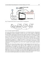
The numerical results for the six cases are summarized in Table 4. In cases 1-5 (balanced
systems), the system power loss and the LBI are highest, and the minimum bus voltage in
the system violates the lower limit of 0.95 per unit. The voltage profile of case 1 is shown in
Fig. 12. It is observed that the voltages at buses 57-65 are below 0.95 p.u. because a large
load of 1,244 kW are drawn at bus 61. Without the four DG units, the system loss would be
673.89 kW. This confirms that DG units can normally, although not necessarily, help reduce
current flow in the feeders and hence contributes to power loss reduction, mainly because
they are usually placed near the load being supplied. In cases 2 to 5, where the feeders are
reconfigured and the voltage constraint is imposed in the optimization process, no bus
voltage is found violated (see Figs.12 and 13).

Case 1 Case 2 Case 3 Case 4 Case 5 Case 6
Sectionalizing switches to be
open
-
12, 20,
52, 61
42, 14,
20, 52, 61
52, 62 13, 52, 63 12, 52 61
Tie switches to be closed -
70, 71,
72, 73
69, 70,

71, 72, 73
72, 73 71, 72, 73 71, 72, 73
Power loss (kW) 586.83 246.33 270.81 302.37 248.40 290.98
Minimum voltage (p.u.) 0.914 0.954 0.954 0.953 0.953 0.965
Load balancing index (LBI) 2.365 1.801 1.748 1.921 1.870 2.273
Number of switching
operations
- 8 10 4 6 6
Table 4. Results of case study
As expected, the system power loss is at minimum in case 2, the LBI index is at minimum in
case 3, and the number of switching operations of switches is at minimum in case 4. It is
obviously seen from case 5 that a fuzzy multiobjective optimization offers some flexibility
that could be exploited for additional trade-off between improving one objective function
and degrading the others. For example, the power loss in case 5 is slightly higher than in case
2 but case 5 needs only 6, instead of 8, switching operations. Although the LBI of case 3 is
better than that of case 5, the power loss and number of switching operations of case 3 are
greater. Comparing case 4 with case 5, a power loss of about 18 kW can be saved from two
more switching operations. It can be concluded that the fuzzy model has a potential for
solving the decision making problem in feeder reconfiguration and offers decision makers
some flexibility to incorporate their own judgment and priority in the optimization model.

Energy Technology and Management

76
The membership value of case 5 for power loss is 0.961, for load balancing index is 0.697 and
for number of switching operations is 0.666.
When the system unbalanced loading is 20% in case 6, the power loss before feeder
reconfiguration is about 624.962 kW. The membership value of case 6 for power loss is 0.840,
for load balancing index is 0.129 and for the number of switching operations is 0.666. The
voltage profile of case 6 is shown in Fig. 14.

1 4 7 10 13 16 19 22 25 28 31 34 37 40 43 46 49 52 55 58 61 64 67 69
0.91
0.92
0.93
0.94
0.95
0.96
0.97
0.98
0.99
1.00
1.01
1.02
1.03
1.04
1.05
Bus
Voltage (p.u.)


Case 1
Case 2
Case 3
Minimum voltage

Fig. 12. Bus voltage profile in cases 1, 2 and 3

1 4 7 10 13 16 19 22 25 28 31 34 37 40 43 46 49 52 55 58 61 64 6769
0.91
0.92
0.93
0.94
0.95
0.96
0.97
0.98
0.99
1.00
1.01
1.02
1.03
1.04
1.05
Bus
Voltage (p.u.)


Case 4
Case 5
Minimum voltage

Fig. 13. Bus voltage profile in cases 4 and 5
Optimal Feeder Reconfiguration with Distributed
Generation inThree-Phase Distribution System by Fuzzy Multiobjective and Tabu Search

77
1 4 7 10 13 16 19 22 25 28 31 34 37 40 43 46 49 52 55 58 61 64 67 69

0.91
0.92
0.93
0.94
0.95
0.96
0.97
0.98
0.99
1.00
1.01
1.02
1.03
1.04
1.05
Bus
Voltage (p.u.)


Phase A
Phase B
Phase C
Minmimum voltage

Fig. 14. Bus voltage profile in cases 6
9. Conclusion
A fuzzy multiobjective algorithm has been presented to solve the feeder reconfiguration
problem in a distribution system with distributed generators. The algorithm attempts to
maximize the satisfaction level of the minimization of membership values of three
objectives: system power loss, load balancing index, and number of switching operations for

tie and sectionalizing switches. These three objectives are modeled by a trapezoidal
membership function. The search for the best compromise among the objectives is achieved
by Tabu search. On the basis of the simulation results obtained, the satisfaction level of one
objective can be improved at the expense of that of the others. The decision maker can
prioritize his or her own objective by adjusting some of the fuzzy parameters in the feeder
reconfiguration problem.
10. References
Kashem, M. A.; Ganapathy V. & Jasmon, G. B. (1999). Network reconfiguration for load
balancing in distribution networks.
IEE Proc Gener. Transm. Distrib., Vol. 146, No. 6,
(November) pp. 563-567.
Su, C. T. & Lee, C. S. (2003). Network reconfiguration of distribution systems using
improved mixed-integer hybrid differential evolution.
IEEE Trans. Power Delivery,
Vol. 18, No. 3, (July) pp. 1022-1027.
Baran, M. E. & Wu, F. F. (1989). Network reconfiguration in distribution systems for loss
reduction and load balancing.
IEEE Trans. on Power Delivery, Vol. 4, No. 2, (April)
pp. 1401-1407.
Kashem, M.A.; Ganapathy V. & Jasmon, G.B. (2000). Network reconfiguration for
enhancement of voltage stability in distribution networks.
IEE Proc Gener. Transm.
Distrib., Vol. 147, No. 3, (May) pp. 171-175.

Energy Technology and Management

78
Gil, H. A. & Joos, G. (2008). Models for quantifying the economic benefits of distributed
generation,
IEEE Trans. on Power Systems, Vol. 23, No. 2, (May) pp. 327-335.

Jones, G. W. & Chowdhury, B. H. (2008). Distribution system operation and planning in the
presence of distributed generation technology.
Proceedings of Transmission and
Distribution Conf
. and Exposition, (April) pp. 1-8.
Quezada, V. H. M.; Abbad, J. R. & Roman, T. G. S. (2006). Assessment of energy distribution
losses for increasing penetration of distributed generation.
IEEE Trans. on Power
Systems
, Vol. 21, No. 2, (May) pp. 533-540.
Carpaneto, E. G.; Chicco, & Akilimali, J. S. (2006). Branch current decomposition method for
loss allocation in radial distribution systems with distributed generation.
IEEE Trans.
on Power Systems
, Vol. 21, No. 3, (August) pp. 1170-1179.
Chung-Fu Chang. (2008). Reconfiguration and capacitor placement for loss reduction of
distribution systems by ant colony search algorithm.
IEEE Trans. on Power Systems,
Vol. 23, No. 4, (November) pp. 1747-1755.
Dengiz, B. & Alabas, C. (2000). Simulation optimization using tabu search.
Proceedings of
Winter Simulation Conf.
, pp. 805-810.
Glover, F. (1989). Tabu search-part
I. ORSA J. Computing, Vol. 1, No.3,
Mori, H. & Ogita, Y. (2002). Parallel tabu search for capacitor placement in radial
distribution system.
Proceedings of Power Engineering Society Winter Meeting Conf.,
Vol. 4, pp 2334-2339.
Das, D. (2006). A fuzzy multiobjective approach for network reconfiguration of distribution

systems.
IEEE Trans. on Power Delivery, Vol. 21, No. 1, (January) pp. 1401-1407
Peponis, G. & Papadopoulos M. (1995). Reconfiguration of radial distribution networks:
application of heuristic methods on large-scale networks.
IEE Proc Trans. Distrib.,
Vol. 142, No. 6. (November) pp. 631-638.
Subrahmanyam, J. B. V. (2009). Load flow solution of unbalanced radial distribution systems.
J. Theoretical and Applied Information Technology, Vol. 6, No. 1, (August) pp. 40-51
Ranjan, R.; Venkatesh, B.; Chaturvedi , A. & Das, D. (2004). Power flow solution of three-
phase unbalanced radial distribution network.
Electric Power Components and
Systems, Vol. 32, No.4, pp.421-433.
Zimmerman, R. D. (1992). Network reconfiguration for loss reduction in three-phase power
distribution system.
Thesis of the Graduate School of Cornell University, May
Zimmermann, H. J. (1987). Fuzzy set decision making, and expert systems.
Kluwer Academic
Publishers
Savier, J. S. & Das, D. (2007). Impact of network reconfiguration on loss allocation of radial
distribution systems.
IEEE Trans. on Power Delivery, Vol. 22, No.4, (October) pp.
2473-2480.
4
Energy Managements in the Chemical and
Biochemical World, as It may be Understood
from the Systems Chemistry Point of View
Zoltán Mucsi, Péter Ábrányi Balogh, Béla Viskolcz and Imre G. Csizmadia
University of Szeged
Hungary
1. Introduction

If anyone compares biochemical and industrial processes from energetic point of view, it
may well be concluded that the bio-production of any living entity exhibits far greater
energy efficiency than any human controlled industrial production. Most of the bio-
reactions take place at the same cell at the same temperature, within a narrow range,
without external heating or cooling system. In contrast to that, industrial chemical processes
usually proceed separately at various reaction temperatures from –80 °C to +200 °C.
Furthermore, these reactions require significantly larger energy input, which is taken in
either as external heating or internal molecular energy of active reagents (high energy
reagents, like acylhalogenides and LiBH
4
), meanwhile the large excess of energy waste,
released during the reaction, must be led away.
Behind the high efficacy of biological processes compared to man-made processes there are
two energetic reasons. At first, biological reactions used to start from low energy
intermediates and proceed by means of very well designed catalysts, such as enzymes,
therefore activation energy gaps are low (Figure 1, green line), consequently reaction can be
carried out at ambient temperature. Secondly, reagents used by living organism, like NAD
+
,
FAD, ATP and other bio-reagents are so effectives under enzymatic conditions, that they
need to store only slightly more than the necessary energy within their structures to carry
out the reaction, resulting low energy waste, or in other word, reagents balance the reaction
energy by their internal molecular energy. Two non-catalyzed laboratory processes (black
dashed and red lines) are compared with a enzyme catalyzed biological process (green line)
schematically in Figure 1 and Table 1. For any reaction to proceed, sufficient reagent has to
be chosen, which at Gibbs free energy level is higher than the Gibbs free energy level of the
product. The Gibbs free energy difference between the row material and product (G
I
→ G
F

)
is called built-in energy. To prepare active reagent from row material, some energy needs to
be invested (G
I
→ G
1
and G
I
→ G
3
). Under laboratory conditions I (black, dashed line),
instead of the addition of high energy and very active reagents, we react only low energy
reagent (at G
1
), therefore thermal energy via increased reaction temperature need to be input
(G
1
→ G
5
), consequently the waste energy is high. In laboratory condition II (red line),
normally high energy and active reagent is reacted via low transition state (G
3
→ G
4
), it does
not require high reaction temperature. However, the overall waste energy remained

Energy Technology and Management
80
significant, due to the large investment energy to prepare active reagents from row

materials. In contrast with the previous processes, biological system (green line) uses low
energy reagents (at G
1
) joint with effective enzyme catalyst (G
I
→ G
2
), therefore the resultant
waste energy is minimal.

Processes
Type of the
process
Invested
energy
Transition
state energy
Waste
energy
Reaction
rate
Product
efficacy
Laboratory I
non-catalysed
low high high
low low
(black dashed) G
1
–G

I
G
5
–G
1
G
F
–G
5
Laboratory II
non-catalysed
high low high
high high
(red line) G
3
–G
I
G
4
–G
3
G
F
–G
4
Biological
catalysed
Low low low
high high
(green) G

1
–G
I
G
2
–G
1
G
F
–G
2
Table 1. Summary of the comparison of two laboratory and a biological processes from
energy management point of view, joining to Figure 1.




Fig. 1. (A) Relative Gibbs free energy profiles for a reaction carried out at laboratory I. (black
dashed line, low energy reagent, non-catalyzed process, therefore high energy transition
state and large energy waste), biological (green line, low energy reagent, enzymatic
catalysis, therefore low energy transition state and low energy waste) and laboratory II.
conditions (red line, high energy reagent, non-catalyzed process, but low energy transition
state and high energy waste). The biological reaction is the most energy efficient due to the
smallest invested and waste-energies. G
I
= initial Gibbs free energy; G
F
= final Gibbs free
energy; from G
1

to G
5
= different Gibbs free energy levels. (B) A schematic comparison of an
incandescent light bulb with a modern ‘energy-saving bulbs’ being in analogy with the
manmade reaction and natural processes.
Energy Managements in the Chemical and Biochemical World,
as It may be Understood from the Systems Chemistry Point of View
81
By symbolic analogy, one may compare the influence of structure on energy loss in many
synthetic reactions to that of an incandescent light bulb; the latter losing (as ‘side product’
wavelengths and heat) ~70 % of energy input to produce the desired product ‘white light’
(Figure 1B). Yield of white light may be improved by optimizing each of the systemic
components, where even shape contributes to efficient excitation of filament-gas to populate
a narrow band of desired energy levels; as in modern ‘energy-saving bulbs’.
Nowadays, in modern organic and medicinal chemistry a typical molecule may involve
several analogous functional groups, which are able to react with a reagent dissimilarly,
resulting in different products, therefore the fast determination or at least estimation of the
reactivity of these functional groups is essential for planning synthetic routes. Nevertheless,
in the case of theoretical methods, which can predict reactivities by modeling the reaction
mechanism, it is typical that behind a seemingly simple chemical reaction, the real
mechanism is quite complex, involving many species in each individual elementary step,
like reactants, reagents, solvent molecules, catalysts, and acid or base as co-reagents [1–5].
All these species should be involved in the calculation to investigate the real and detailed
mechanism, in order to obtain a correct and accurate view of the reaction taking place in a
real media. In fact, determination of the minimal size of the appropriate chemical model
(e.g. number of explicit solvent molecules necessary) is very difficult, time and resource
consuming [1]. Moreover, an incorrect chemical model provides not only inaccurate energy
values, but frequently absolutely wrong or opposite results, questioning the competence of
theoretical methods in the applied science [1]. Reactions taking place in media usually
require the consideration of a base or an acid as catalyst together with many solvent

molecules in an appropriate 3D arrangement [1,2,5]. Taking into consideration of all of these
criteria, it seems nearly impossible to model even a simple acylation reaction. It was
demonstrated earlier that the computation of one or a few, easily and quickly computable
quantum mechanical (QM) descriptors, such as aromaticity [6–9], amidicity [10–12],
carbonylicity,[13,14] olefinicity,[15–17] and others can predict properly and somewhat
quantitatively certain reactivity and selectivity issues. The global and complex view of these
descriptors was defined as the concept of systems chemistry [18], wherein molecules are
described as strategically located functional components within molecular frameworks,
‘valued’ at more than their components’ sum, acting in unison to effect efficient energy
management.
2. The concept and methodology of systems chemistry
2.1 General remarks
Every organic structure and their energy content can be modeled at three levels of
organization. This deconvolution of the total energy into three components is illustrated by
Figure 2. The first level takes into consideration only the σ skeleton of a molecule, the
energy content of this level can be calculated by the sum of the average sigma bond type.
The second level summarizes the π scaffold, summing up the π energy content of the double
bonds (i.e. double bond energy – single bond energ). It is known that adjacent double bonds
get into interactions by overlapping between their atomic orbitals. However, the estimation
of the energy content of the resonance level is not trivial. In simpler cases, where the number
and the types of the σ and the π-bonds do not change the resonance energy is turned out to
be a reliable measure of the overall relative energetic of the process. In order to measure it, a
novel concept and therefore a novel discipline was defined, wherein molecules are


Energy Technology and Management
82

Fig. 2. A schematic illustration of how the internal molecular energy may be deconvoluted
to σ, π and resonance energy.

described as frameworks of strategically located functional components within molecular
frameworks, acting in unison to effect efficient energy management. The term ‘Systems
Chemistry’ effectively serves to define the phenomena of an assembly of atoms and
functional groups (a molecule) having systemic properties ‘valued’ at more than their
component sum. Systems Chemistry focuses on the framework of component functional
groups and atoms within a given molecule acting in unison to orchestrate a variety of
chemical phenomena. Molecular properties, such as reactivity and stability, are a result of
the relative spatial orientation(s) of constituent atoms, mediated by environmental and
statistical factors (e.g. solvent and concentration/bulk, respectively). Systems Chemistry is a
discipline wherein component functionalities are not segregated, in a reductionist fashion,
but rather where they are considered as integrated parts of a whole system of interacting
functional groups; yet, reductionist component resolution is retained.
This implies that functional molecular systems are more than just assemblies of atomic and
functional components. To attain Nature’s efficiency, one must approach chemical
phenomena as systems rather than as single entities. Systems Chemistry has in-hand the
types and locations of organic functional groups (e.g. ortho, meta, para substitutions, catalyst-
ligand identities) and aims to quantifying their relationships and influence on one another.
Coupling between components of a chemically or biologically important molecule, such as
aromatic rings, amide groups, olefins, carbonyls and metal-ligands, are central to the
Energy Managements in the Chemical and Biochemical World,
as It may be Understood from the Systems Chemistry Point of View
83
molecules’ chemical efficiency. With the quantification of these couplings in mind, we
recently introduced the molecular descriptors: aromaticity,[6] amidicity,[10]
carbonylicity,[13] olefinicity,[15] each of which in a surrogate thermodynamic function,
contributing to the characterization of the mechanisms by which Nature fine-tunes and
stores reaction energies to attain hyper-efficiency.
2.2 Aromaticity
Chemical structures and transition states are often influenced by aromatic stabilizing or
antiaromatic destabilizing effects, which are not easy to characterize either experimentally

or theoretically. The exact description and precise quantification of the aromatic
characteristics of ring structures is difficult and requires special theoretical investigation. A
novel, yet simple method to quantify both aromatic and antiaromatic qualities on the same
linear scale, by using the enthalpy of hydrogenation reaction of the compound has been
examined. A reference hydrogenation reaction is also considered on a corresponding non-
aromatic reference compound in order to cancel all secondary structure destabilization
factors, such as ring strain or double bond strain. From these data the relative enthalpy of
hydrogenation may easily be calculated [6]:
ΔΔH
H2
= ΔH
H2
(examined)– ΔH
H2
(reference). (1)
In the present work concept, the ΔΔH
H2
value of benzene defines the perfect or completely
aromatic character (+100%), while the closed shell of the singlet cyclobutadiene represents
maximum antiaromaticity (–100%).
Aromaticity and antiaromaticity are characterised by a common and universal linear scale
based on the heat of hydrogenation (ΔH
H2
(I), Eq. 2; Figure 3) when cyclobutadiene (1) and
benzene (2) are considered as –100% and +100%, respectively. This methodology compares the
hydrogenation reaction of the examined compound [3→6, ΔH
H2
(I), Eq. 2] with that of a
properly chosen reference reaction [9→12, ΔH
H2

(II), Eq. 3]. The difference between the two
enthalpy values [ΔΔH
H2
(AR), Eq. 4] is transformed to aromaticity percentage (AR %; Eq. 5),
which is the basis of the calculation of the resonance enthalpy [H
RE
(AR); Eq. 6]. Some aromatic
compounds may exhibit larger aromaticity values, than 100%, meaning to a larger resonance
enthalpy (RE) inside the system. Typical case is the double ring naphthalene and its analogues,
where this larger value is the sum of the resonance enthalpies of the two rings.
ΔH
H2
(I) = H[6] – {H[3] + H(H
2
)} (2)
ΔH
H2
(II) = H[12] – {H[9] + H(H
2
)} (3)
ΔΔH
H2
(AR) = ΔH
H2
(I) – ΔH
H2
(II) (4)
AR % = m
AR
ΔΔH

H2
(AR) + b
AR
(5)
H
RE
(AR) = AR % / m
AR
(6)
The various compounds for which aromaticity and antiaromaticity values were determine
form a “spectra” of such aromatic/antiaromatic characters are illustrated by Figure 4.
Interesting examples can be found in phosphorous organic compounds [7–9,19], one of them
is exemplified in Figure 5. The aromaticity of phospholes was questionable for a long time
and the commonly accepted view was that they have a very weak aromatic character. The


Energy Technology and Management
84

Reference reactionExamined reaction
1
4710
25
811
-100%
100%
H
2
H
2

H
2
H
2
Degree of aromaticity
()
n
()
m
()
n
()
m
()
n
()
m
()
n
()
m
ΔH
H2
(I)
H
2
ΔH
H2
(II)
H

2
36
912

Fig. 3. ΔH
H2
vales calculated for an antiaromatic and aromatic species.


Fig. 4. Combined aromaticity and antiaromaticity spectrum with some representative
compounds.
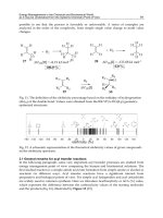
weak aromaticity may be due to the pyramidal geometry around the P atom since the lone
electron pair cannot effectively participate in the delocalization. Several studies revealed
that contrary to the stability of phosphole (13), phosphole oxide derivatives (14) exhibit an
unusual instability. The phosphole oxides (14) obtained on oxidation of the phospholes (13),
undergo a Diels-Alders type [4+2] dimerization reaction to afford 15 (upper line of Figure
5). Other experimental findings revealed that an other phosphole derivative 16 is stable for
days, but their oxidized derivative 17 is unstable under the same conditions and is
Energy Managements in the Chemical and Biochemical World,
as It may be Understood from the Systems Chemistry Point of View
85
rearranged to 18 (lower line of Figure 5). The instability of 17 was explained by the existing
weak antiaromaticity [9,19].


Fig. 5. ΔH
H2
vales calculated for selected antiaromatic and aromatic species containing
phosphorous.
2.3 Carbonylicity and amidicity

The carbonyl group is one of the most pervasive moieties in organic, bioorganic and industrial
chemistry. Ketons, aldehydes as well as carboxylic acids, their halogenides, amides, esters, acyl
anhydrides and other derivatives are also so-classified, commonly found in peptides/proteins,
lipids/membranes and other biologically active compounds, such as Penicillin, drugs and
toxins. They may be characterized as being very stable and resilient (amides, esters, acids), as
well as very reactive systems (carboxyl acid halogenids, and thiol derivatives). There are
numerous examples in the field of organic and biochemistry, where the carbonyl derivatives
undergoes nucleophilic addition reaction, such as esterification, transesterification, amidation,
transamidation, anhydride formation, aldol addition, among others. Examples also include the
near-spontaneous or enzymatic hydrolysis of ester and amide bonds. Reduction of the
carbonyl group by complex metal hydrides has significant synthetic importance in obtaining
various alcohols, amines and other compounds (Figure 6). The large variability in the chemical
reactivity of the carbonyl group may be attributed to the potential for fine-tuning of the bond
strength, facilitated by attached substituent groups. Stronger conjugation, implies a larger
contribution of resonance stabilization (lowering overall energy), with an associated increase
in system stability. The extent of conjugation, predetermines its specific chemical reactivity;
analogous to the situation in amide systems [13].

Energy Technology and Management
86

Fig. 6. A schematic illustration of the variety of reactions of carbonyl derivatives.
The large variability in the chemical reactivity of the amide bond may be attributed to the
potential for fine-tuning of the bond strength, facilitated by the attached substituent groups.
The amide bond strength of a general amide compound, as illustrated by its associated
resonance structures, determines its specific chemical reactivity; essential to the biological
activity of biochemical compounds. A stronger amide bond is more resistant to attack by
nucleophilic agents (e.g. HO
–
, H

2
O, amines, metal hydrides or the hydroxyl groups of
serine–proteases), whereas a weaker amide bond is correspondingly more reactive. For a
stronger amide bond, the conjugation between N and the C of the carbonyl group is more
extensive, meaning that the contribution of the two most significant resonance structures are
more closely balanced between the two structures, than in a weaker amide bond. In the case
where there is no significant conjugation, the preferred resonance structure is represented
by the left structure in the box in Fig. 6. [10].
2.3.1 Amidicity and carbonylicity percentages and its resonance enthalpies (AM%
and CA %):
The “amidicity scale”, quantifying amide bond (Figure 7) strength on a linear scale, based
on the computed enthalpy of hydrogenation [ΔH
H2
(AM); Eq. 7; Figure 8-TOP] of the
compound examined, comparing to reference compounds 19 and 20. The ΔH
H2
(AM) value
for dimethylacetamide (19) is used to define perfect amidic character (Eq. 8.; AM % =
+100%), while azaadamantane-2-on (20) represents complete absence of amidic character
(AM % = 0%) [10]. The amidicity value is transformed to the resonance enthalpy [H
RE
(AM);
Eq. 9]. However, amidicity is not limited to the values between 0% and 100%. Some amide
compounds exhibit extreme amidicity values, either below 0% or above 100%, and referring
to the cases when the amide bond may be weaker than that in 20 or stronger than that in 19,
respectively.
ΔH
H2
(AM) = H[22] – {H[21] + H(H
2

)} (7)
AM % = m
AM
ΔH
H2
(AM) + b
AM
(8)
H
RE
(AM) = AM % / m
AM
(9)
Energy Managements in the Chemical and Biochemical World,
as It may be Understood from the Systems Chemistry Point of View
87

Fig. 7. A schematic illustration of the occurance of an amide bond within protein secondary
structures.


Fig. 8. The definition of the amidicity (TOP) and carbonylicity percentages (BOTTOM)
based on the enthalpy of hydrogenation (ΔH
H2
) of the carbonyl group. Values were obtained
from the B3LYP/6-31G(d,p) geometry-optimized structures. In structure 22 and 26, the O–
C–X–R
3
and the H–O–C–X dihedral angles are chosen to be in the anti orientation.

Energy Technology and Management
88
Analogously, the “carbonylicity scale”, quantifying carbonyl bond strength on a linear scale,
based on the computed enthalpy of hydrogenation [ΔH
H2
(CA); Eq. 10; Figure 8-BOTTOM]
of the compound examined, comparing to reference compounds 23 and 24. The ΔH
H2
(CA)
value for formiate anion (23) is used to define perfect conjugation (Eq. 11.; CA % = +100%),
while formaldehyde (24) represents complete absence of a conjugation (CA % = 0%) [13]. To
calculate the carbonylicity value of compound 25 can be calculated by the hydrogenation
reaction to 26, using Eq. 10–12. The carbonylicity value is transformed to the resonance
enthalpy [H
RE
(CA); Eq. 12]. Here the carbonylicity value is also not limited to the values
between 0% and 100%.
ΔH
H2
(CA) = H[25] – {H[26] + H(H
2
)} (10)
CA % = m
CA
ΔH
H2
(CA) + b
CA
(11)
H

RE
(CA) = CA % / m
CA
(12)
Figure 9 shows, in a combined fashion the amidicity (TOP) and carbonylicity (BOTTOM)
scale. Note that the two set of values represent different scales, than the amidicity is a
special section of the carbonylicity scale.
Amidicity percentage for example is able to predict whether a transamidation reaction is
taking place under the given conditions or not [10–12] and it can also point out the most
reactive amide bond of a molecule. It was shown that carbonyl groups exhibiting a lower
amidicity value are more reactive toward nucleophilic reagents (like amines) than carbonyl
groups having a larger value. Moreover, when more products can be deduced it was
demonstrated that the difference between the sum of amidicity percentages of products and
the sum of those values in the reactants indicates the direction of a transamidation reaction.
If this difference is positive, the reaction is energetically favored, while in the case of a
negative value the reaction is disadvantageous from the driving force point of view. The
reaction route, where the sum of amidicity percentages for products is larger than that for
other possible reaction routes, is predicted to be the favorable one.
A very similar conclusion was drawn for acyl transfer reactions using carbonylicity as the
descriptor [13]. It should be noted, however, that these simple views of the reaction do not
consider the kinetic consequences, which sometimes perturb the simplest and quickest
conclusion. For example, as presented in an earlier work [13], in acyl transfer reactions it is
not enough to find the lowest carbonylicity value, but one of the carbonyl groups should
also be a good leaving group.
2.4 Olefinicity
The olefinic group, illustrated in Figure 10, may be considered as one of the most important
moieties in the organic and bioorganic chemistry. Substituted olefines, such as enamines,
vinyl eters and other derivatives can be ranked among this category. Most of them are
common in the field of the biochemistry such as proteins, lipids, nucleinic acids and other
biologically active compounds like drugs and toxins. Their chemical reactivity may be

characterised as very stable and resistant chemical systems, (simple olefines), as well as very
active and reactive compounds (enamines, vinyl esters, etc.). There are numerous examples
in the field of organic and biochemistry, where the olefinic derivatives undergo electrophilic
or nucleophilic reactions [15].
Energy Managements in the Chemical and Biochemical World,
as It may be Understood from the Systems Chemistry Point of View
89
















Fig. 9. A schematic representation of the theoretical amidicity and carbonylicity values of
given compounds on the carbonylicity and amidicity spectrum, illustrating, that the
amidicity spectrum is a small section of the carbonylicity spectrum.

Energy Technology and Management
90
The large variability in the chemical reactivity of the olefin group may be attributed to the

potential fine-tuning ability of the bond conjugation, facilitated by the attached substituent
groups. The extent of conjugation of a general olefin compound, as illustrated by its associated
resonance structures (Figure 10), predetermines its specific chemical reactivity [15].



Fig. 10. Some selected typical reactions of the olefinic moiety.
2.4.1 Olefinicity percentage and its resonance enthalpy (OL %):
The “olefinicity scale”, quantifying alkene bond strength (Figure 11) on a linear scale, based
on the computed enthalpy of hydrogenation [ΔH
H2
(OL); Eq. 13] of the compound examined
(29), comparing to reference compounds 27 and 28 (Eq. 14) [15]. The ΔH
H2
(OL) value for
allyl anion (27) is used to define equivalent conjugation (OL % = +100%), while ethylene (28)
represents complete absence of conjugation (OL % = 0%), by Eq. 15. This olefinicity value is
transformed to resonance enthalpy [H
RE
(OL); Eq. 15].
ΔH
H2
(OL) = H[T] – {H[S] + H(H
2
)} (13)
OL % = m
OL
ΔH
H2
(OL) + b

OL
(14)
H
RE
(OL) = OL % / m
OL
(15)
3. Energetic study of industrial and biochemical reactions
Due to the enormously large variety of chemical reactions, in this chapter only acyl transfer
reactions, including transamidation and reduction-oxidation reactions are exemplified,
which are also essential both in industrial chemistry and biochemistry. In order to
understand the energy flow and determine the direction of such reactions, thermodynamic
selection rule and driving force should be clarified. Based on Systems Chemistry approach,
measuring numerically the resonance energy of functional groups inside the molecule, a
relatively simple protocol is provided for practicing organic chemists to predict the outcome
of an experiment. The change of specific values over the course of a reaction made it