transformer engineering design and practice 1_phần 7 pptx
Bạn đang xem bản rút gọn của tài liệu. Xem và tải ngay bản đầy đủ của tài liệu tại đây (698.37 KB, 62 trang )
169
5
Stray Losses in Structural
Components
The previous chapter covered the theory and fundamentals of eddy currents. It
also covered in detail, the estimation and reduction of stray losses in windings,
viz., eddy loss and circulating current loss. This chapter covers estimation of
remaining stray losses, which predominantly consist of stray losses in structural
components. Various countermeasures required for the reduction of these stray
losses and elimination of hot spots are discussed.
The stray loss problem becomes increasingly important with growing
transformer ratings. Ratings of generator transformers and interconnecting auto-
transformers are steadily increasing over last few decades. Stray losses of such
large units can be appreciably high, which can result in higher temperature rise,
affecting their life. This problem is particularly severe in the case of large auto-
transformers, where actual impedance on equivalent two-winding rating is higher
giving a very high value of stray leakage field. In the case of large generator
transformers and furnace transformers, stray loss due to high current carrying
leads can become excessive, causing hot spots. To become competitive in the
global marketplace it is necessary to optimize material cost, which usually leads to
reduction in overall size of the transformer as a result of reduction in electrical and
magnetic clearances. This has the effect of further increasing stray losses if
effective shielding measures are not implemented. Size of a large power
transformer is also limited by transportation constraints. Hence, the magnitude of
stray field incident on the structural parts increases much faster with growing
rating of transformers. It is very important for a transformer designer to know and
estimate accurately all the stray loss components because each kW of load loss
may be capitalized by users from US$750 to US$2500. In large transformers, a
reduction of stray loss by even 3 to 5 kW can give a competitive advantage.
Copyright © 2004 by Marcel Dekker, Inc.
Chapter 5170
Stray losses in structural components may form a large part (>20%) of the total
load loss if not evaluated and controlled properly. A major part of stray losses
occurs in structural parts with a large area (e.g., tank). Due to inadequate shielding
of these parts, stray losses may increase the load loss of the transformer
substantially, impairing its efficiency. It is important to note that the stray loss in
some clamping elements with smaller area (e.g., flitch plate) is lower, but the
incident field on them can be quite high leading to unacceptable local high
temperature rise seriously affecting the life of the transformer.
Till 1980, a lot of work was done in the area of stray loss evaluation by
analytical methods. These methods have certain limitations and cannot be applied
to complex geometries. With the fast development of numerical methods such as
Finite Element Method (FEM), calculation of eddy loss in various metallic
components of the transformer is now easier and less complicated. Some of the
complex 3-D problems when solved by using 2-D formulations (with major
approximations) lead to significant inaccuracies. Developments of commercial 3-
D FEM software packages since 1990 have enabled designers to simulate the
complex electromagnetic structure of transformers for control of stray loss and
elimination of hot spots. However, FEM analysis may require considerable
amount of time and efforts. Hence, wherever possible, a transformer designer
would prefer fast analysis with sufficient accuracy so as to enable him to decide on
various countermeasures for stray loss reduction. It may be preferable, for regular
design use, to calculate some of the stray loss components by analytical/hybrid
(analytically numerical) methods or by some formulae derived on the basis of
one-time detailed analysis. Thus, the method of calculation of stray losses should
be judiciously selected; wherever possible, the designer should be given
equations/curves or analytical computer programs providing a quick and
reasonably accurate calculation.
Computation of stray losses is not a simple task because the transformer is a
highly asymmetrical and three-dimensional structure. The computation is
complicated by
- magnetic non-linearity
- difficulty in quick and accurate computation of stray field and its effects
- inability in isolating exact stray loss components from tested load loss values
- limitations of experimental verification methods for large power transformers
Stray losses in various clamping structures (frame, flitch plate, etc.) and the tank
due to the leakage field emanating from windings and due to the field of high
current carrying leads are discussed in this chapter. The methods used for
estimation of these losses are compared. The effectiveness of various methods
used for stray loss control is discussed. Some interesting phenomena observed
during three-phase and single-phase load loss tests are also reported.
Copyright © 2004 by Marcel Dekker, Inc.
Stray Losses in Structural Components 171
5.1 Factors Influencing Stray Losses
With the increase in ratings of transformers, the proportion of stray losses in the
load loss may increase significantly. These losses in structural components may
exceed the stray losses in windings in large power transformers (especially
autotransformers). A major portion of these stray losses occurs in structural
components with a large area (e.g., tank) and core clamping elements (e.g.,
frames). The high magnitude of stray flux usually does not permit designers to
disregard the non-linear magnetic characteristics of steel elements. Stray losses in
structural steel components depend in a very complicated manner on the
parameters such as the magnitude of stray flux, frequency, resistivity, type of
excitation, etc.
In the absence of hysteresis and non-linearity of magnetic characteristics, the
expression for the eddy loss per unit surface area of a plate, subjected to (on one of
its surfaces) a magnetic field of r.m.s. value (H
rms
), has been derived in Chapter 4
as
(5.1)
Hence, the total power loss in a steel plate with a permeability µ
s
can be given in
terms of the peak value of the field (H
0
) as
(5.2)
This equation assumes a constant permeability. It is necessary to take into account
the non-linear magnetic saturation effect in structural steel parts because their
surfaces are often saturated due to the skin effect. Non-linearity of magnetic
characteristics can be taken into account by a linearization coefficient as explained
in Section 4.4. Thus, the total power loss with the consideration of non-linear
characteristics can be given by
(5.3)
The term a
l
in the above equation is the linearization coefficient. Equation 5.3 is
applicable to a simple geometry of a plate excited by a tangential field on one of its
sides. It assumes that the plate thickness is sufficiently larger than the depth of
penetration (skin depth) so that it becomes a case of infinite half space. For
magnetic steel, as discussed in Section 4.4, the linearization coefficient has been
taken as 1.4 in [1]. For a non-magnetic steel, the value of the coefficient is
1(i.e.,a
l
=1).
Copyright © 2004 by Marcel Dekker, Inc.
Chapter 5172
5.1.1 Type of surface excitation
In transformers, there are predominantly two kinds of surface excitation as shown
in figure 5.1. In case (a), the incident field is tangential (e.g., bushing mounting
plate). In this case, the incident tangential field is directly proportional to the
source current since the strength of the magnetic field (H) on the plate surface can
be determined approximately by the principle of superposition [2]. In case (b), for
estimation of stray losses in the tank due to a leakage field incident on it, only the
normal (radial) component of the incident field (
φ
) can be considered as
proportional to the source current. The relationship between the source current
and the tangential field component is much more complicated. In many analytical
formulations, the loss is calculated based on the tangential components (two
orthogonal components in the plane of plate), which need to be evaluated from the
normal component of the incident field with the help of Maxwell’s equations.
The estimated values of these two tangential field components can be used to
find the resultant tangential component and thereafter the tank loss as per equation
5.3.
Let us use the theory of eddy currents described in Chapter 4 to analyze the
effect of different types of excitation on the stray loss magnitude and distribution.
Consider a structural component as shown in figure 5.2 (similar to that of a
winding conductor of figure 4.5) which is placed in an alternating magnetic field
in the y direction having peak amplitudes of H
1
and H
2
at its two surfaces. The
structural component can be assumed to be infinitely long in the x direction.
Further, it can be assumed that the current density J
x
and magnetic field intensity
H
y
are functions of z only. Proceeding in a way similar to that in Section 4.3 and
assuming that the structural component has linear magnetic characteristics, the
diffusion equation is given by
Figure 5.1 Types of excitation
Copyright © 2004 by Marcel Dekker, Inc.
Stray Losses in Structural Components 173
(5.4)
The solution of this equation is
Hy=C
1
e
γz
+C
2
e
-γz
(5.5)
where γ is propagation constant given by equation 4.39, viz. γ=(1+j)/
δ
,
δ
being
the depth of penetration or skin depth. Now, for the present case the boundary
conditions are
H
y
=H
1
at z=+b and H
y
=H
2
at z=-b (5.6)
Using these boundary conditions, we can get expressions for the constants as
(5.7)
Substituting these values of constants back into equation 5.5 we get
(5.8)
Since ∇×H=J and J=σE, and only the y component of H and x component of J are
non-zero we get
(5.9)
(5.10)
Figure 5.2 Stray loss in a structural component
Copyright © 2004 by Marcel Dekker, Inc.
Chapter 5174
In terms of complex vectors, the (time average) power flow per unit area of the
plate (in the x-y plane) can be calculated with the help of Poynting’s theorem [3]:
(5.11)
Substituting the values of H
y
and E
x
from equations 5.8 and 5.10, the value of eddy
loss per unit area of the plate can be calculated. Figure 5.3 shows the plot of the
normalized value of eddy loss, P/(H
2
/2σδ), versus the normalised plate thickness
(2b/δ) for three different cases of the tangential surface excitation.
Case 1 (H
1
=H and H
2
=0): As expected, the eddy loss for this case decreases with
the increase in plate thickness until the thickness becomes 1 to 2 times the skin
depth. This situation resembles the case in a transformer when a current carrying
conductor is placed parallel to a conducting plate (mild steel tank/ pocket). For
this case (see figure 5.3), the normalised active power approaches unity as the
thickness and hence the ratio 2b/δ increases. This is because it becomes a case
similar to an infinite half space, where the power loss equals H
2
/(2σδ). It is to be
remembered that H, H
1
and H
2
denote peak values.
Figure 5.3 Eddy Loss in a structural plate for different surface excitations
Copyright © 2004 by Marcel Dekker, Inc.
Stray Losses in Structural Components 175
The plot also shows that the active power loss is very high for a thin plate. A
qualitative explanation for this phenomenon can be given with reference to figure
5.4 (a). Consider a contour C shown in the figure. By applying Ampere’s circuital
law on the contour we obtain
(5.12)
Noting that H is only in the y direction with H
1
=H and H
2
=0, the equation
simplifies to
HL=I
As the thickness 2b decreases, the same amount of current passes through a
smaller cross section of the plate and thus through a higher resistance, resulting in
more loss.
Case 2 (H
1
=H
2
=H): Here, the eddy loss increases with the increase in the plate
thickness. This situation arises in lead terminations/bushing mounting plates,
where a current passes through holes in the metallic plates. In this case, as the
thickness increases, normalized active power loss approaches the value of 2
because, for 2b/
δ
>>1, the problem reduces to that of two infinite half-spaces, each
excited by the peak value of field (H) on their surfaces. Therefore, the total loss
adds up to 2 per-unit. As the thickness decreases, the active power loss decreases
in contrast with Case 1. As shown in figure 5.4 (b), the currents in two halves of
the plate are in opposite directions (as forced by the boundary conditions of H
1
and H
2
). For a sufficiently small thickness, the effects of these two currents tend to
cancel each other reducing the loss to zero.
Case 3 (H
1
=-H
2
=H): Here, the eddy loss decreases with the increase in thickness.
For very high thickness (much greater than the skin depth), the loss approaches
the value corresponding to two infinite half-spaces, i.e., H
2
/(
σδ
). As the thickness
decreases, the power loss approaches very high values. For the representation
Figure 5.4 Explanation for curves in Figure 5.3
Copyright © 2004 by Marcel Dekker, Inc.
Chapter 5176
given in figure 5.4 (c), an explanation similar to that for Case 1 can be given. The
application of Ampere’s circuital law gives double the value of current (i.e.,
2HL=I) as compared to Case 1. Hence, as the thickness (2b) decreases, the current
has to pass through a smaller cross section of the plate and thus through a higher
resistance causing more loss.
In the previous three cases, it is assumed that the incident magnetic field
intensity is tangential to the surface of a structural component (e.g., bushing
mounting plate). If the field is incident radially, the behavior of stray loss is
different. Based on a number of 2-D FEM simulations involving a configuration in
which the leakage field from the windings is radially incident on a structural
component (e.g., tank or flitch plate), the typical curves are presented in figure
5.5. The figure gives the variation of loss in a structural component as the
thickness is increased, for three different types of material: magnetic steel, non-
magnetic steel and aluminum. The curves are similar to those given in [4] wherein
a general formulation is given for the estimation of losses in a structural
component for any kind of spatial distribution of the incident magnetic field.
Let us now analyse the graphs of three different types of materials given in
figure 5.5.
Figure 5.5 Loss in different materials for radial excitation
Copyright © 2004 by Marcel Dekker, Inc.
Stray Losses in Structural Components 177
1) Magnetic steel: One can assume that the magnetic steel plate is saturated due to
its small skin depth. Hence, the value of relative permeability corresponding to the
saturation condition is taken (µ
r
=100). With
σ
=7×10
6
mho/m, we get the value of
skin depth as 2.69 mm at 50 Hz. It can be seen from the graph that the power loss
value reaches a maximum in about two skin depths and thereafter remains
constant. This behavior is in line with the theory of eddy currents and skin depth
elaborated in Chapter 4. Since eddy currents and losses are concentrated at the
surface only, increasing the plate thickness beyond few skin depths does not
change the effective resistance offered to the eddy currents and hence the loss
remains constant (at a value which is governed by equation 4.74).
2) Aluminum: In case of aluminum with µ
r
=1 and
σ
=29×10
6
mho/m, the skin
depth at 50 Hz is 13.2 mm. It can be observed from the graph that the loss first
increases with thickness and then reduces. The phenomenon can be analyzed
qualitatively from the supply end as an equivalent resistive-inductive circuit. For
small thickness (thin plates), it becomes a case of resistance-limited behavior (as
discussed in Section 4.5.1) and the effective resistance is larger compared to the
inductance. Hence, the equivalent circuit behaves as a predominantly resistive
circuit, for which the loss can be given as P=(V
2
/R), where V is the supply voltage.
An increase of the thickness of the aluminum plate leads to a decrease of
resistance, due to the increased cross section available for the eddy-currents, and
hence the loss increases. This is reflected in a near-linear increase in losses with
the increase of plate thickness.
Upon further increase of the plate thickness, the resistance continues to
decrease while the inductance gradually increases, and the circuit behavior
changes gradually from that of a purely resistive one to that of a series R–L circuit.
The power loss undergoes a peak, and starts to decrease as the circuit becomes
more inductive. Finally, when the thickness is near or beyond the skin depth, the
field and eddy currents are almost entirely governed by the inductive effects
(inductance-limited behavior). The field does not penetrate any further when the
plate thickness is increased. The equivalent resistance and inductance of the
circuit become independent of the increase in the plate thickness. The power loss
also approaches a constant value as the thickness increases significantly more than
the skin depth making it a case of infinite half space. Since the product (
σ
·
δ
) is
much higher for the aluminum plate than that for the mild steel plate, the constant
(minimum) value of loss for the former is much lower (the loss is inversely
proportional to the product (
σ
·
δ
) as per equation 4.74). The curves of aluminum
and mild steel intersect at about 3 mm (point A).
3) Non-magnetic stainless steel: For the non-magnetic steel plate, the behavior is
similar to that of the aluminum plate, both being non-magnetic materials. The
curve is more flat as compared to aluminum as the skin depth of stainless steel is
quite high. For a typical grade of stainless steel material with relative permeability
of 1 and conductivity of 1.136×10
6
mho/m, the skin depth is 66.78 mm at 50 Hz.
Copyright © 2004 by Marcel Dekker, Inc.
Chapter 5178
Another difference is that as the thickness is increased, loss approaches a constant
value higher than the aluminum plate but lower than the magnetic steel plate since
the product (
σ
·
δ
) for stainless steel lies between that of mild steel and aluminum.
The intersection point (B) of the curves for stainless steel and aluminum occurs at
about 5 mm and the intersection point (C) of the curves for stainless steel and mild
steel occurs at about 10 mm. The location of intersection points depends on the
configuration being analyzed and the nature of the incident field.
With the increase in the plate thickness, the values of losses in the mild steel
(MS), aluminum (AL) and stainless steel (SS) plates stabilize to 12.2 kW/m, 1.5
kW/m and 5.7 kW/m respectively for particular values of currents in the windings.
For large thickness, it becomes a case of infinite half space and the three loss
values should actually be in proportion to (1/
σδ
) for the same value of tangential
component of magnetic field intensity (H
0
) on the surface of the plate (as per
equation 4.74). The magnitude and nature of eddy currents induced in these three
types of plates are different, which makes the value of H
0
different for these cases.
Also, the value of H
0
is not constant along the surface (as observed from the FEM
analysis). Hence, the losses in the three materials are not in the exact proportion of
their corresponding ratios (1/
σδ
). Nevertheless, the expected trend is there; the
losses follow the relationship (loss)
MS
>(loss)
SS
>(loss)
AL
since (1/
σδ
)
MS
>(l/
σδ
)
SS
>(1/
σδ
)
AL
.
A few general conclusions can be drawn based on the above discussion:
1) When a plate made of non-magnetic and highly conductive material (aluminum
or copper) is used in the vicinity of field due to high currents or leakage field from
windings, it should have thickness at least comparable to its skin depth (13.2 mm
for aluminum and 10.3 mm for copper at 50 Hz) to reduce the loss in it to a low
value. For the field due to a high current, the minimum value of loss is obtained for
a thickness of [5],
(5.13)
For aluminum (with
δ
=13.2 mm), we get the value of t
min
as 20.7 mm at 50 Hz. The
ratio t
min
/
δ
corresponding to the minimum loss value is 1.57. This agrees with the
graph of figure 5.3 corresponding to Case 1 (assuming that tangential field value
H
2
≅0 which is a reasonable assumption for a thickness 50% more than
δ
), in
which the minimum loss is obtained for the normalized thickness of 1.57. For the
case of radial incident field also (figure 5.5), the loss reaches a minimum value at
the thickness of about 20 mm. For t<(0.5×
δ
), the loss becomes substantial and
may lead to overheating of the plate. Hence, if aluminum or copper is used as an
electromagnetic (eddy current) shield, then it should have sufficient thickness to
eliminate its overheating and minimize the stray loss in the structural component
Copyright © 2004 by Marcel Dekker, Inc.
Stray Losses in Structural Components 179
(shielded by it). Sufficient thickness of a shield ensures that its effective resistance
is close to the minimum value.
2) Since the skin depth of mild steel (2.69 mm) is usually much less than the
thickness required from mechanical design considerations, one may not be able to
change its thickness to control the eddy loss. Hence, either magnetic shunts (made
of low reluctance steel material) or electromagnetic shields (aluminum or copper)
are used to minimize the stray losses in structural components made of mild steel
material in medium and large transformers.
3) From figure 5.5, it is clear that the loss in a stainless steel plate is less than a
mild steel plate for lower values of thickness. Hence, when a structural component
is made of stainless steel, its thickness should be as small as possible (permitted
from mechanical design considerations) in order to get a lower loss value. Thus, if
a mild steel flitch plate is replaced by a stainless steel one, the stray loss in it is
lower only if its thickness is about 10 mm or lower.
5.1.2 Effect of load, temperature and frequency
Generally, it is expected that the load loss test is conducted at the rated current. For
large power transformers the tested load loss value at a lower current when
extrapolated to the rated condition in the square proportion of currents may result
in a value less than the actual one. This is because the stray losses in structural
components, which form an appreciable part of the total load loss in large power
transformers, may increase more than the square proportion. With the increase in
winding currents and leakage field values, saturation effects in the (mild steel)
material used for structural components increase. If magnetic or electromagnetic
shield is not adequately designed, it becomes less effective at higher currents
increasing stray losses. The exponent of current for stray losses may even be of the
order of 2.3 to 2.5 instead of 2 in such cases [2]. Hence, depending upon the
proportion of stray losses in the total load loss, the latter will be higher than that
extrapolated with the exponent of 2. Hence, it is preferable to do the load loss test
at the rated current for large transformers. If the test plant is having some
limitation, the test can be done at a current less than the rated value subject to the
agreement between user and manufacturer.
It should be noted that equation 5.2 or 5.3 can be used for a plate excited by a
tangential field on one side, the plate thickness being sufficiently larger than the
skin depth so that it becomes a case of infinite half space. By using an analytical
approximation for the magnetization curves of a commonly used mild steel
material, equation 5.2 or 5.3 for the power loss per unit surface area in a massive
steel element subjected to a tangential field of H
0
at the surface, can be rewritten in
terms of the source current I as [6]
(5.14)
Copyright © 2004 by Marcel Dekker, Inc.
Chapter 5180
The above equation is valid when H
0
is proportional to I, which is true for example
in the case of bushing mounting plates. The current exponent of 1.5 is reported in
[4] for the loss in bushing mounting plates.
For stray losses in magnetic steel plates subjected to the field of high current
carrying bars (leads), the exponent of current is slightly less than 2. The exponent
is a function of distance between the bar and the plate [7] (=1.975-0.154log
10
h,
where h is distance from center of bar to plate surface in inches). For aluminum
plates, the current exponent can be taken as 2 [7,8].
The power loss per unit area for an incident flux which is radial in nature
(incident normally on the plate), is given by [6]
(5.15)
Equation 5.15 is applicable to the case of tank plate subjected to the stray leakage
field emanating from windings. The inter-winding gap flux is proportional to the
current in windings. It has been reported [9] that in the case of tank plate being
penetrated by a part of stray (leakage) field originating from windings, the relation
between this radial field and the winding current is
(5.16)
where
κ
is in the range of 0.8 to 0.9. Hence, equation 5.15 can be re-written in terms
of current as
(5.17)
where
η
, the exponent of current, is in the range of 2.2 to 2.5, which is in line with
the value of 2.3 given in [2]. Hence, some stray loss components increase with the
load current having an exponent greater than 2. Since these losses generally do not
form the major part of load losses (if adequate shielding is done) and other stray
losses vary with the current exponent of 2 or less than 2, the load loss dependence
on the current is not much different than the square proportion. This is particularly
true when the load loss test is done at or below the rated currents. Under
overloading conditions, however, the load loss may increase with the current
having an exponent higher than 2.
Losses due to high current field (e.g., in bushing mounting plate) vary in direct
proportion of as per equation 5.14. From equation 5.17, it is clear that the
stray losses in tank vary in almost the inverse proportion of resistivity and square
proportion of frequency. Since the eddy losses in windings are also inversely
proportional to resistivity (see equation 4.94), the total stray losses may be
assumed to vary in the inverse proportion of resistivity (because the winding eddy
losses and tank stray losses form the major part of stray losses for most of the
transformers). For simplicity in calculations, they are assumed to be varying in the
inverse proportion of the resistivity of winding conductor. Thus, the total stray
losses in transformers can be related to resistivity as
Copyright © 2004 by Marcel Dekker, Inc.
Stray Losses in Structural Components 181
(5.18)
Since metals have positive temperature coefficient of resistance (resistivity
increases with temperature), the stray losses can be taken to vary in the inverse
proportion of temperature. If the load loss is guaranteed at 75°C, the stray loss
component of the measured load loss at temperature t
m
is converted to 75°C by the
formula (when the copper conductor is used in windings)
(5.19)
For aluminum conductor the constant 235 is replaced by 225. Contrary to stray
losses, the DC I
2
R loss in windings varies in direction proportion of resistivity and
hence the temperature. Therefore, for the copper conductor,
(5.20)
The I
2
R loss at t
m
(obtained by converting the value of I
2
R loss corresponding to
DC resistance test done at temperature t
r
to temperature t
m
) is subtracted from the
measured value of load loss at t
m
to calculate P
stray_
t
m
. In order to calculate I
2
R loss
at t
m
, the average winding temperature should be accurately determined. This is
done by taking the average of top and bottom cooler temperatures. A substantial
error may occur if, after oil processing and filtration cycles at about 50 to 60°C, a
sufficient time is not provided for oil to settle down to a lower temperature (close
to ambient temperature). In such a case, the temperature of windings may be quite
different than the average of top and bottom cooler temperatures. Hence, it is
preferable to wait till the oil temperature settles as close to the ambient
temperature or till the difference between the top and bottom oil temperatures is
small enough (the difference should not exceed 5°C as per ANSI Standard
C57.12.90–1993) for accurate measurements. For the forced oil cooling system, a
pump may be used to mix the oil to minimize the difference between top and
bottom oil temperatures.
Regarding the effect of frequency variation on the total stray losses, it can be
said that since the eddy loss in windings is proportional to the square of frequency,
the stray loss in tank is proportional to frequency with an exponent less than 2 as
per equation 5.17, and the stray loss due to the field of high current varies with f
0.5
as per equation 5.14, the total stray loss varies with frequency with an exponent x,
whose value depends on the proportion of these losses in the total stray loss.
(5.21)
Copyright © 2004 by Marcel Dekker, Inc.
Chapter 5182
If the winding eddy loss and stray losses in all structural components are treated
separately, the winding eddy loss (stray loss in windings) is taken to be varying
with frequency in the square proportion, whereas remaining stray losses can be
assumed to vary with frequency having an exponent close to 1. According to IEC
61378 Part-1, 1997, Transformers for industrial applications, the winding eddy
losses are assumed to depend on frequency with the exponent of 2, whereas stray
losses in structural parts are assumed to vary with frequency with the exponent of
0.8. The frequency conversion factors for various stray loss components are
reported and analyzed in [10].
For a transformer subjected to a non-sinusoidal duty, at higher frequencies the
skin depth is lower than the thickness of the winding conductor. Hence, the
relationship given by equation 4.90 or 5.1 is more valid (frequency exponent of
0.5) instead of that given by equation 4.94 (frequency exponent of 2 when
thickness is less than the skin depth). Therefore, at higher frequencies the
frequency exponent for the winding eddy loss reduces from 2 to a lower value
[11].
5.2 Overview of Methods for Stray Loss Estimation [12]
After having seen basic theory of stray loss in structural components, we will now
take a look at how methods of computation of stray losses have evolved from
approximate 2-D analytical methods to present day advanced 3-D numerical
methods.
5.2.1 Two-dimensional methods
A method is given in [13] for estimating leakage field, in which any kind of
current density distribution can be resolved into space harmonics by a double
Fourier series. The leakage field distribution obtained in the core window by this
method can be used to calculate the approximate value of losses in flitch plate and
first step of the core (in addition to eddy loss in windings). A two-dimensional
Axisymmetric finite element formulation based on magnetic vector potential is
used in [14] to obtain the tank losses. A computer program based on 2-D FEM
formulation for skin effect and eddy current problems is presented in [15]. The
formulation is suitable for both Cartesian and Axisymmetric 2-D problems. In
[16], analogy between magnetic field equations for 2-D Cartesian and
Axisymmetric problems is presented, and usefulness of this analogy for numerical
calculations has been elaborated. The relation between finite element and finite
difference methods is also clarified. Results of measurement of flux densities and
eddy currents on a 150 MVA experimental transformer are reported. In [17], a 2-
D finite element formulation based on magnetic vector potential is presented,
which takes into account the varying distance between the winding and tank (due
to 3-D geometry) by a correction factor. The 2-D FEM is used to get a static
magnetic field solution in [18], and losses in tank are calculated by analytical
Copyright © 2004 by Marcel Dekker, Inc.
Stray Losses in Structural Components 183
formulae. The paper has reported test results of tank losses with magnetic and
eddy current shielding. The geometric parameters affecting tank losses are
explained through graphs. The need is emphasized in [19] for analyzing the stray
losses as a complete system and not on an individual component basis. For
example, placement of magnetic shunts on tank surface has the effect of reducing
stray losses in clamping elements of the core since the leakage field gets more
oriented towards the tank. The magnetic tank shunts also increase the radial field
at the ends of outer winding and may increase the winding eddy loss if the width
of its conductor is high enough to compensate the reduction in eddy loss due to
reduced axial field at the ends. A number of 2-D FEM simulations are done to
understand the effect of tank shields (magnetic/eddy current) on the other stray
loss components (winding, flitch plate, frame and core edge losses). The
simulations have shown that the effectiveness of magnetic shunts is quite
dependent on the permeability of material indicating that the magnetic shunts
should have adequate thickness so that their permeability does not reduce due to
saturation.
In this era of 3-D calculations, 2-D methods are preferred for routine
calculations of stray losses. These 2-D methods can be integrated into transformer
design optimization programs which need reasonably accurate determination of
stray losses.
5.2.2 Three-dimensional analytical formulations
A quasi 3-D formulation is given in [20], which obtains the radial flux density
distribution on the tank wall by using method of images. The calculation of flux
density does not consider the effect of the tank eddy currents on the incident field.
This assumption is made to simplify the analytical formulation. From this radially
incident peak value of the flux density (say in the z direction), the tangential
components of magnetic field intensity (H
x
and H
y
) are calculated from Maxwell’s
equations. The resultant peak value is used to calculate the
power loss per unit area with the assumption of step-magnetization characteristics
(similar to the theory given in Section 4.4). The total losses in the tank are
calculated by integration carried over the entire area. The method given in [21]
calculates 3-D magnetic flux density distribution on the tank wall using a 2-D
solution for one phase of a three-phase transformer.
These analytical methods may not get easily applied to complicated tank
shapes and for finding the effects of tank shielding accurately. For such cases 3-D
numerical methods are commonly used.
5.2.3 Three-dimensional numerical methods
Advent of high speed and large memory computers has made possible the
application of numerical methods such as FEM, Finite Difference Method,
Copyright © 2004 by Marcel Dekker, Inc.
Chapter 5184
Boundary Element Method, etc., for the calculation of 3-D fields inside a
transformer and accurate estimation of stray losses in structural components.
Boundary Element Method (BEM) is more suitable for open boundary
problems involving structural parts of non-magnetic stainless steel, where it is
difficult to determine the boundary conditions [22,23]. For such open boundary
conditions, some researchers have used [24] Integral Equation Method (IEM). In
order to make the grid (mesh) generation easier, IEM with surface impedance
modeling is proposed in [25]. Improved T-⍀ (electric vector potential-magnetic
scalar potential) formulation is used in [26], wherein the total problem region is
divided into source, non-conductive and conductive regions simplifying
computational efforts.
An overview of methods for eddy current analysis is presented in [27]. The
paper compares methods based on differential formulation (analytical, finite
difference method, reluctance network method), integral formulation (volume
integral, boundary element method), and variational methods (weighted residual,
FEM) on attributes such as accuracy, ease of use, practicality and flexibility. The
advantages of BEM for transient and open boundary problems are enumerated in
the paper. There is continuous ongoing development in 3-D numerical
formulations (which started gaining importance in 1980s) to improve their
modeling capabilities and accuracy for the analysis of eddy currents.
After having seen the different approaches for the calculation of stray losses,
we will now discuss in detail each stray loss component and its control.
5.3 Core Edge Loss
Core edge loss is the stray loss occurring due to flux impinging normally
(radially) on core laminations. The amount and path of leakage field in the core
depends on the relative reluctances of the alternative magnetic circuits. Load
conditions of the transformer also have significant influence; the phase angle
between the leakage field and magnetizing field decides the loading of the
magnetic circuit and the total core losses during operation at site. During factory
tests, the leakage flux path in the core depends largely on whether the inner or
outer winding is short-circuited as explained in Section 5.12.2. The incident
leakage flux density on the limb and clamping elements is quite appreciable in
case of generator transformers due to relative closeness of the limb from the inter-
winding gap as compared to autotransformers. Hence, there are more possibilities
of hot spots being generated in these parts in generator transformers. However, the
stray loss magnitude may be of the same order in generator transformers and
autotransformers due to more leakage field in autotransformers on equivalent two
winding basis.
In large transformers, the radially incident flux may cause considerable eddy
currents to flow in the core laminations resulting in local hot spots. The flux
penetration phenomenon is quite different in a laminated core structure as
Copyright © 2004 by Marcel Dekker, Inc.
Stray Losses in Structural Components 185
compared to a solid one. In a solid block of finite dimensions, the eddy currents
tending to concentrate at the edges can complete their path through the side faces,
and the field is confined to the surface (skin depth) in all faces. In the laminated
case, there is restriction to the flow of eddy currents and the field penetrates much
deeper as compared to the solid case. The leakage flux penetration into the
laminated core poses an anisotropic and three-dimensional non-linear field
problem. The problem is formulated in terms of electric vector potential and
magnetic scalar potential (T-Ω formulation) in [28]. The solution is expressed in
the form of three different characteristic modes, two associated with the core
surfaces and the third describing the flux penetration into the interior. All the three
modes are represented in a network model by complex impedances, and then the
current distribution and losses are derived from the solution of the network. The
core discontinuities (holes) are accounted by change of appropriate impedances.
Thus, the method provides a means of studying effects of core steps, holes, ducts
and discontinuities (due to lapped joints). The network has to be modified with
any change in the geometry or type of excitation. The formulation in the paper has
been verified on two experimental models of a core [29,30]. Approximate
formulae for finding the loss and temperature rise of a core due to an incident field
are also given. The effect of type of flitch plate (magnetic or non-magnetic) on the
core edge loss is also explained. A non-magnetic (stainless steel) flitch plate
increases the core edge loss since it allows (due to its higher skin depth) the flux to
penetrate through it to impinge on the laminations. Hence, although the use of
non-magnetic flitch plate may reduce the loss in it (assuming that its thickness is
sufficiently small as explained in Section 5.1.1), the core edge loss is generally
increased.
The first step of the core is usually slit into two or three parts to reduce the core
edge loss in large transformers. If the stack height of the first step of the core is less
than about 12 mm, slitting may have to be done for the next step also. The use of
a laminated flitch plate for large generator transformers and autotransformers is
preferable since it also acts as a magnetic shunt (as described in Section 5.5).
The evaluation of exact stray loss in the core poses a challenge to transformer
designers. With the developments in 3-D FEM formulations with features of
anisotropic modeling (of permeability and conductivity), the computational
difficulties can be overcome now.
5.4 Stray Loss in Frames
Frames (also called as yoke beams), serving to clamp yokes and support windings,
are in vicinity of stray magnetic field of windings. Due to their large surface area
and efficient cooling, hot spots seldom develop in them. The stray loss in frames
has been calculated by Finite Difference Method and an analytical method in [31].
The loss in frames made up of mild steel, aluminum and non-magnetic steel are
compared. It has been shown that the losses in frame and tank have mutual effect
Copyright © 2004 by Marcel Dekker, Inc.
Chapter 5186
on each other. Non-magnetic steel is not recommended as a material for frames. It
is expensive, difficult to machine and stray losses will be lower only if its
thickness is sufficiently small. A quick and reasonably accurate calculation of the
frame loss can be done by using 3-D Reluctance Network Method (RNM) [32].
The numerical methods such as FEM are also commonly used.
The loss in frames due to leakage field can be reduced by either aluminum
shielding or by use of non-metallic platforms for supporting the windings. In
distribution transformers, the stray loss in the tank may not be much since the
value of leakage field is low. But the loss in frames due to currents in low voltage
leads running parallel to them can be significant. For example, the current of a star
connected LV winding of a 2 MVA, 11/0.433 kV transformer is 2666.67 A, which
can result into stray loss in the frames of the order 1 kW (which is substantial for
a 2 MVA transformer). Non-metallic frames can be used (after thorough
assessment of their short circuit withstand capability) for eliminating the stray
loss.
Another way of minimizing this loss is by having go and return arrangement of
LV winding leads passing close to the frame. These two leads can be either firmly
supported from the frame or they can pass through a hole made in the frame as
shown in figure 5.6. The net field responsible for eddy current losses in the
metallic frame is negligible as the two currents are in opposite directions.
A single lead may be allowed to pass through a hole in the frame with a non-
magnetic insert (e.g., stainless steel material with high resistivity) as shown in
figure 5.7 upto a certain value of current.
In power transformers, sometimes a frame of non-magnetic material (stainless
steel) is used. As explained in Section 5.1.1, its thickness should be as small as
mechanically possible; otherwise its loss may exceed the corresponding value for
frame made of (magnetic) mild steel material.
Figure 5.6 Go and return arrangement Figure 5.7 Non-magnetic insert
Copyright © 2004 by Marcel Dekker, Inc.
Stray Losses in Structural Components 187
5.5 Stray Loss in Flitch Plates
Stray flux departing radially through the inner surface of windings hits fittings
such as flitch plates mounted on the core. On the surface of the flitch plate (lying
on the outermost core-step of limbs for holding core laminations together
vertically), the stray flux density may be much higher than that on the tank. Hence,
although the losses occurring in a flitch plate may not form a significant part of the
total load loss of a transformer, the local temperature rise can be much higher due
to high value of incident flux density and poorer cooling conditions. The loss
density may attain levels that may lead to a hazardous local temperature rise if the
material and type of flitch plate are not selected properly. The higher temperature
rise can cause deterioration of insulation in the vicinity of flitch plate, thereby
seriously affecting the transformer life.
There are a variety of flitch plate designs being used in power transformers as
shown in figure 5.8. For small transformers, mild steel flitch plate without any
slots is generally used because the incident field is not large enough to cause hot
spots. As the incident field increases in larger transformers, a plate with slots at the
top and bottom ends can be used (where the incident leakage field is higher).
Sometimes, flitch plates are provided with slots in the part corresponding to the
tap zone in taps-in-body designs. These slots of limited length may be adequate if
the incident field on the flitch plates is not high. Fully slotted plates are even
better, but they are weak mechanically, and their manufacturing process is a bit
more complicated. The plates can be made of non-magnetic stainless steel having
high resistivity only if their thickness is small as explained in Section 5.1.1. When
the incident leakage field on the flitch plate is very high, as in large generator
transformers, the best option would be to use a laminated flitch plate. It consists of
a stack of CRGO laminations, which are usually held together by epoxy molding
to make the assembly mechanically strong. The top and bottom ends of
laminations are welded to solid (non-magnetic) steel pads which are then locked
Figure 5.8 Types of flitch plates
Copyright © 2004 by Marcel Dekker, Inc.
Chapter 5188
to the frames. A laminated flitch plate not only minimizes its own eddy loss but it
also acts as a magnetic shunt reducing the loss in the first step of the core.
The literature available on the analysis of flitch plate loss is quite scarce. An
approximate but practical method for calculation of the loss and temperature rise of
a flitch plate is given in [4], which makes certain approximations based on the
experimental data given in [33]. The field strength at the inner edge of LV winding
is assumed to vary periodically with a sinusoidal distribution in the space along the
height of the winding, and the non-sinusoidal nature is accounted by multiplying
the loss by a factor. The eddy current reaction is neglected in this analytical
formulation. For a fully slotted flitch plate, the formulation is modified by considering
that the plate is split into distinct parts. A more accurate 2-D/3-D FEM analysis is
reported in [34], in which many limitations of analytical formulations are overcome.
The paper describes details of statistical analysis, orthogonal array design of
experiments, used in conjunction with 2-D FEM for quantifying the effect of various
factors influencing the flitch plate loss. This Section contains results of authors’
paper [34] © 1999 IEEE. Reprinted, with permission, from IEEE Transactions on
Power Delivery, Vol. 14, No. 3, July 1999, pp. 996–1001. The dependence of flitch
plate loss on the axial length of windings, core-LV gap, winding to yoke clearance
and LV-HV gap is observed to be high. The flitch plate loss varies almost linearly
with LV-HV gap. A quadratic surface derived by multiple regression analysis can
be used by designers for a quick but approximate estimation of the flitch plate loss.
The loss value obtained can be used to decide type (with slots/without slots) and
material (magnetic mild steel/non-magnetic stainless steel) of the flitch plate to control
its loss and avoid hot spots. The effectiveness of number and length of slots in reducing
losses can be ascertained accurately by 3-D field calculations. In the paper, in-depth
analysis of eddy current paths has been reported for slotted mild steel and stainless
steel flitch plates, having dimensions of 1535 mm×200 mm×12 mm, used in a single-
phase 33 MVA, 220/132/11 kV autotransformer.
For this analysis, a mild steel (MS) flitch plate with µ
r
=1000 and σ= 4×10
6
mho/m has been studied. The corresponding skin depth is 1.1 mm at 50 Hz. The
results obtained are summarized in table 5.1. The loss values shown are for one
fourth of the complete plate.
Case number Description Loss in watts
1 No slots 120
2 1 slot throughout 92
3 3 slots throughout 45
4 7 slots throughout 32
5 1 slot of 400mm length 100
6 3 slots of 400mm length 52
7 7 slots of 400mm length 45
Table 5.1 Loss in MS flitch plate
Copyright © 2004 by Marcel Dekker, Inc.
Stray Losses in Structural Components 189
The loss for the ‘7 slots throughout’ case is approximately 4 times less than that
of the ‘no slots’ case. Theoretically, the loss is proportional to the square of width,
hence for n slots, the loss should reduce approximately by a factor of (n+1), i.e., 8
(if a plate width of 3w is divided by 2 slots into 3 plates of width w, then loss will
theoretically reduce by a factor of (3w)
2
divided by 3w
2
, i.e., 3). The reason for this
discrepancy can be explained as follows. The pattern of eddy currents is complex
in a mild steel material. Eddy loss in it has two components, viz. loss due to radial
incident field, and the other due to axial field (the incident radial flux changes its
direction immediately once it penetrates inside the plate due to very small skin
depth). This phenomenon is evident from the eddy current pattern in the plate
cross section, taken at 0.5 mm from the surface facing the windings (figure 5.9 and
figure 5.10). There is hardly any change in the eddy current pattern in this cross
section after the introduction of slots. The direction of eddy currents suggests the
predominance of axial field at 0.5 mm from the surface. Hence, there are eddy
current loops in the thickness of the plate as shown in figure 5.11. These are the
reasons for the ineffectiveness of slots in the MS plate, which is responsible for the
fact that the reduction of losses is not by a factor of 8.
Figure 5.9 Eddy currents in MS plate with no slots
Figure 5.10 Eddy currents in MS plate with 3 slots
Copyright © 2004 by Marcel Dekker, Inc.
Chapter 5190
For a non-magnetic stainless steel (SS) flitch plate (µ
r
=1,
σ
=1.13×10
6
mho/m),
due to its large penetration depth (67 mm at 50 Hz), the incident field penetrates
through it and hits the core laminations. This phenomenon is evident from the
eddy current pattern at the plate cross section taken at 0.5 mm from the surface
(figures 5.12 and 5.13). There is an appreciable distortion in the eddy current
pattern after the introduction of slots.
Figure 5.11 Eddy currents across thickness of MS plate with 3 slots
Figure 5.12 Eddy currents in SS plate with no slots
Figure 5.13 Eddy currents in SS plate with 3 slots
Copyright © 2004 by Marcel Dekker, Inc.
Stray Losses in Structural Components 191
The direction of eddy currents indicates the predominance of radial field at the
cross section, 0.5 mm from the surface. There are no eddy current loops in
thickness of the plate (see figure 5.14). These are the reasons for the effectiveness
of slots in the SS plate. The eddy current loops are parallel to the surface (on which
the flux in incident) indicating that the eddy loss in the SS plate is predominantly
due to the radial field. Hence, the slots in the SS plate are more effective as
compared to the MS plate. This means that the loss should reduce approximately
by a factor of (n+1). From the first two results given in table 5.2, we see that the
reduction in the loss is more (12 times) than expected (8 times). This may be due
to fact that each slot is 5 mm wide causing a further reduction in the loss due to the
reduced area of conduction.
Due to higher resistivity of SS, the losses in the SS plate are lower than the MS
plate. If results from tables 5.1 and 5.2 are compared for the ‘no slots’ case, it can
be seen that the SS plate loss is not significantly lower than the MS plate loss for
12 mm thickness. For a higher thickness, the loss in the SS plate may exceed the
loss in the MS plate, which is in line with the graphs in figure 5.5. It shows that in
order to get lower losses with SS material, its thickness should be as small as
possible with due considerations to mechanical design requirements. With the SS
plate, shielding effect is not available. Hence, although losses in the flitch plate are
reduced with SS material, the stray loss in the first step of the core may increase
substantially if it is not split. Therefore, thicker flitch plates with a low incident
flux density should be of MS material.
A laminated flitch plate (consisting of M4 grade CRGO laminations) has also
been analyzed through 3-D FEM analysis by taking anisotropy into account. The
direction along the flitch plate length is defined as soft direction and other two
directions are defined as hard directions. The loss value obtained for the laminated
flitch plate is just 2.5 watts, which is quite lower than the SS plate. Hence,
laminated flitch plates are generally used for large power transformers,
particularly generator transformers, where the incident flux density is quite high.
Figure 5.14 Eddy currents across thickness in SS plate with 3 slots
Case Number Description Loss in watts
1 No slots 98
2 7 slots throughout 8
3 7 slots 400 mm long 11
4 3 slots 400 mm long 17
Table 5.2 Losses in SS flitch plate
Copyright © 2004 by Marcel Dekker, Inc.
Chapter 5192
The eddy loss distribution obtained by 3-D FEM electromagnetic analysis is
used for estimation of the temperature rise of the flitch plate by 3-D FEM thermal
analysis [34,35]. The heat generation rates (watts/m
3
) for various zones of the
flitch plate are obtained from the 3-D FEM electromagnetic analysis. The
computed temperatures have been found to be in good agreement with that
obtained by measurements. Thus, the method of combined 3-D electromagnetic
FEM analysis and thermal FEM analysis can be used for the analysis of eddy loss
and temperature rise of a flitch plate. Nowadays, commercial FEM software
packages are available having multi-physics capability. Hence, the temperature
rise can be found more easily without manual interface between the
electromagnetic FEM analysis and thermal FEM analysis.
5.6 Stray Loss in Tank
The tank stray loss forms a major part of the total stray loss in large power
transformers. Stray flux departing radially from the outer surface of winding gives
rise to eddy current losses in transformer tank walls. Though the stray flux density
in the tank wall is low, the tank loss may be high due to its large area. Hot spots
seldom develop in the tank, since the heat is carried away by the oil. A good
thermal conductivity of the tank material also helps to mitigate hot spots. The
stray loss in tank is controlled by magnetic/eddy current shields.
Methods for estimation of tank loss have evolved from approximate analytical
methods to present day more accurate three-dimensional numerical methods. The
radial incident flux density at various points on the tank is found in [36] by
neglecting the effect of eddy currents on the incident field. It is assumed that the
ampere-turns of windings are concentrated at the longitudinal center of each
winding as a current sheet, and the field at any point on the tank is calculated by
superimposition of the fields due to all windings. The tank loss is calculated using
the estimated value of the radial field at each point. The analytical formulation in
[37] determines the field in air without the presence of tank, from the construction
of the transformer and the currents in windings. Based on this field and the
coefficient of transmission, the tangential component of the magnetic field
strength on the inner surface of the tank is determined. The specific power loss at
a point is then calculated by using the value of active surface resistance of the tank
material. The total losses are determined by summing the specific losses on the
surface of the tank. The analytical method, presented in [38], takes into account
the hysteresis and non-linearity by using complex permeability. A current sheet,
the sum of trigonometric functions in between the core and tank (both treated as
infinite half space), represents mmf of windings. The calculated value of the radial
component of the flux density at the tank surface is corrected by a coefficient
accounting for the influence of eddy currents. The tank loss is found by Poynting’s
vector. The method can be applied for a specific tank shape only. The effect of
magnetic/eddy current shields on the tank wall is not accounted in the method.
The analytical approach in [39] expresses the incident flux density (obtained by
Copyright © 2004 by Marcel Dekker, Inc.
Stray Losses in Structural Components 193
any method) on the tank in terms of double Fourier series. Subsequently, after
getting the field and eddy current distribution within the tank plate, the loss is
evaluated by using volume integral. The results are verified by an experimental
set-up in which a semi-circular electromagnet is used to simulate the radial
incident field on the tank plate.
Thus, since the 1960s the research reported for calculation of tank loss has
been mainly concentrating on various analytical methods involving intricate
formulations, which approximate the three-dimensional transformer geometry to
simplify the calculations. Transformer designers prefer fast interactive design
with sufficient accuracy to enable them to decide the method for reducing tank
stray losses. Reluctance Network Method [1] can fulfill the requirements of very
fast estimation and control of the tank stray loss. It is based on a three-dimensional
network of reluctances. The reluctances are calculated from various geometrical
dimensions and electrical parameters of the transformer. There are two kinds of
elements: magnetic resistances for non-conductive areas and magnetic
impedances for conductive parts. The first ones are calculated purely from the
geometrical dimensions of the elements, whereas the latter ones take into account
analytically the skin effect, eddy current reactions with phase shift, non-linear
permeability inside solid metals, and the effect of eddy current shields (if placed
on the tank wall). Hence, the method is a hybrid method in which the analytical
approach is used (for the portion of the geometry involving eddy currents) in
conjunction with the numerical formulation.
The equivalent reluctance of the solid iron can be determined with the help of
the theory of eddy currents explained in Chapter 4. For a magnetic field applied on
the surface of solid iron in the y direction, and assuming that it is function of z only
(figure 5.15), the amplitude of flux per unit length in the x direction is
(5.22)
Figure 5.15 Equivalent reluctance for tank
Copyright © 2004 by Marcel Dekker, Inc.