Manual for Soil Analysis-Monitoring and Assessing Soil Bioremediation Phần 6 pot
Bạn đang xem bản rút gọn của tài liệu. Xem và tải ngay bản đầy đủ của tài liệu tại đây (389.41 KB, 37 trang )
7 Feasibility Studies for Phytoremediation of Metal-Contaminated Soil 175
7.3.8
Conclusions
The combined chemo-phytostabilization method has the following advan-
tages:
• Phosphateasusedinthemethoddecreasestheconcentrationofbivalent
heavy metals in roots and shoots, and their bioavailable fraction in
leachates, and also improves plant cover density.
• Further, phosphat e thus i ntroduced in soil m ay fa cilitate t he propagation
of Deschampsia in the third year of growth by enhancing production of
seeds, which germinate on bare soil between the tufts.
• The procedure supports the growth of the root system and makes it
stronger, resulting in increases of up to 70% water retention and reduced
metal migration.
• The growth of D. caespitosa is improved in the process at the expense of
thegrowthrateofCar dam inopsis sp. This is a positive phenomenon, be-
cause high heavy-metal accumulation rates in Cardam inopsis sp. shoots
results in a potential introduction of heavy metals into the food chain.
• Metalmigrationtolowersoillevelsisdecreasedbytheprocedureas
a result of metal-chemical binding and the development of a strong plant
cover .
• An optimization study to evaluate phosphorus addition to the soil and
satisfactory plant gro wth remains tobedone, and thepriceof theadditiv e
isalsoamatterofconcern.
• Phosphate used as a fertilizer for metal contaminated soils in very high
concentration is considered disadvantageous as it causes saturation with
phosphate in the upper soil layers. This can lead to phosphate leaching.
Phosphate use is therefore limited t o areas with a deep water table where
groundwater pollution by phosphate is unlikely, and where the greater
benefit of obtaining healthy plant cover is unlikely to be achieved.
• Phosphateisnotrecommendedforarsenic-pollutedsoils,ascompetition
between arsenate and phosphate can provoke increased arsenic levels in
plants, causing risks of food-chain propagation and accumulation.
Acknowledgements. The authors wish toexpress their thanks toMr. Laymon
Gray of Florida State University for his editorial contribution to this paper.
176 A. Sas-Nowosielska et al.
References
Berti WR, Cunningham SD, Cooper EM (1998) Case studies in the field – in-place inac-
tivation and phytorestoration of Pb-contaminated sites. In: Vangronsveld J and Cun-
ningham SD (eds) Metal-contaminated soils: in situ inactivation and phytorestoration.
Springer-Verlag, Berlin Heidelberg and RG Landes Co, Georgetown, TX, USA, pp 235–
248
Blaylock MJ, Salt DE, Dushenkov S, Zakharova O, Gussman C, Kapulnik Y, Ensley BD,
Raskin I (1997) Enhanced accumulation of Pb in Indian mustard by soil-applied chelat-
ing agents. En viron Sci Technol 31:860–865
Brooks RR (1998) Phytochemistry of hyperaccumulators. In: Brooks RR (ed) Plants that
hyperaccumulate heavy metals. Cab International, Wallingford, O xon, UK, pp 15–53
Houba VJG, Van der Lee JJ, Novozamsky I (1995) Soil analysis procedures, other procedures
(Soil and plant analysis, Part 5b). Dept Soil Sci Plant Nutr, Wageningen Agricultural
University, pp 217
ISO 11265 (1994) Soil quality – Determination of the specific electric conductivity
ISO 11464 (1993) Soil quality – Pr etreatment of samples for physico-chemical analyses
ISO 13536 (1995) Soil quality – Determination of the potential cation exchange capacity and
exchangeable cations using barium chloride solution buffered at pH
= 8.1
ISO 7888 (1985) Water quality – Determination of electrical conductivity
ISO/CD/10381–5 (1995) Soil quality – Sampling
ISO/DIS 10390 (1993) Soil quality – Determination of pH
ISO/DIS 11047 (1994) Soil quality – Determination of cadmium, chromium, cobalt, copper,
lead, manganese, nickel and zinc. Flame and electromatic thermal atomic absorption
spectrometric methods
ISO/DIS 11466 (1995) Soil quality – Extraction of trace metals and heavy metals soluble in
aqua regia
Knox AS, Seaman J, Adriano DC, Pierzynski G (2000) Chemophytostabilization of metals in
contaminated soils. In: Wise DL, Trantolo DJ, Cichon EJ, Inyang HI, Stottmeister U (eds)
Bioremediation of contaminated soils. Marcel Dekker, Inc, New York, Basel, pp 811–
836
Knox AS, Seaman JC, Mench MJ, Vangronsveld J (2001) Remediation of metal- and
radionuclides-contaminated soils by in situ stabilization techniques. In: Iskandar IK
(ed) Environmental restoration of metal-contaminated soils. Lewis Publ, Boca Raton,
London, New York, Washington, DC, pp 21–60
Kucharski R, Sas-Nowosielska A, Dushenkov S, Kuperberg JM, Pogrzeba M, Malkowski E
(1998) Technology of phytoextraction of lead and cadmium in Poland. Pro blems and
achievements. In: Symposium Proceedings, Warsaw’98, Fourth Int Symposium and
Exhibition on Environmental Contamination in Central and Eastern Europe, pp 55
Kucharski R, Sas-Nowosielska A, Kryñski K (2000) Amendment application technology
for phytoextraction. In: Symposium Program, Prague 2000, Fifth Int Symposium and
Exhibition on Environmental Contamination in Central and Eastern Europe, Abstract,
p 376
Kucharski R, Sas-Nowosielska A, Kuperberg M, Bocian A (2004) Survey and assessment.
How urbanization and industries influence water quality. In: Integrated watershed man-
agement – ecohydrology & phytotechnology, manual. UN Educational, Scientific and
Cul tural Organization, Venice, Italy, pp 45–60
Li YM, Chaney L (1998) Case studies in the field – industrial sites: phytostabilization of zinc
smelter-contaminated sites: the Palmerton case. In: Vangronsveld J, Cunningham SD
(eds) Metal-con taminated soils: in situ inactivation and phytor estoration. Springer-
Verlag Berlin Heidelberg, and RG Landes Co, Georgetown, TX, USA, pp 197–210
7 Feasibility Studies for Phytoremediation of Metal-Contaminated Soil 177
McGrathSP, Dunham SJ,Correl RL (2000)Potentialforphytoextraction of zinc andcadmium
from soils using hyperaccumulator plants. In: Terry N, Banuelos G (eds) Phytoremedi-
ation of contaminated soil and water. Lewis Publ, Florida, pp 1–13
Salt DE, Smith RD, Raskin I (1998) Phytoremediation. Annu Rev Plant Physiol Plant Mol
Biol 49:643–668
Sas-Nowosielska A, Kucharski R, Korcz M, Kuperberg M, Malkowski E (2001) Optimizing
of land characterization for phytoextraction of heavy metals. In: Gworek B, Mocek A
(eds) Element cycling in the environment, bioaccumulation – toxicity – prevention,
Monograph, vol 1. Instytut Ochrony Œrodowiska, Warsaw, Poland, pp 345–348
Sas-Nowosielska A, Kucharski R, Malkowski E, Pogrzeba M, Kuperberg M, Kryñski K (2004)
Phytoextraction crop disposal – an unsolved problem. Environ Pollution 128:373–379
Vangronsveld J, Cunningham SD (1998) Introduction to the concept. In: Vangronsveld J,
Cunningham SD (eds) Metal-contaminated soils: i n situ inactivation and phytorestora-
tion. Springer-Verlag, Berlin Heidelberg, and RG Landes Co, Georgetown, TX, USA,
pp 1–15
Vangronsveld J, Van Assche F, Clijsters H (1995) Reclamation of a bare industrial area
contaminated by non-ferrous metals: in situ metal immobilization and revegetation.
Environ Pollution 87:51–59
8
Quantification of Hydrocarbon
Biodegradation Using Internal Markers
R oger C. Prince, Gregory S. Douglas
■
Introduction
Objectives. Soil contamination is invariably heterogeneous, and monitor-
ing the loss of contaminant during bioremediation is often frustrated by
this heterogeneity. But if the initial source of contamination was relatively
homogeneous, it is possible to identify biodegradation as the selective loss
of the most biodegradable components, while more recalcitrant molecules
are conserved. Measuring the concentrations of a series of compounds us-
ing gas c hromatography (GC) coupled with mass spectrometry (MS), often
in the selected ion monitoring (SIM) mode, allows this to be achieved with
high precision.
Hopanes have proven to be useful conserved internal markers for fol-
lowing the biodegradation of crude oil contamination (Prince at al. 1994),
trimethylphenanthrenes for following the biodegradation of diesel fuel
(Douglas et al. 1992), and 2,2,3,3-tetramethylbutane and 1,1,3-trimethyl-
cyclopentane for following the anaerobic biodegradation of gasoline and
condensate (Townsend et al. 2004). Undoubtedly, there are many other
compounds that could be used. Even if the “conserved” internal marker
is itself eventually degraded, this will have the effect of underestimating
the extent of biodegradation of compounds referred to it, making the ap-
proach a co nservative one. The principal requirements are that the samples
under consideration initially had the same contaminant, and that the com-
pound chosen as the “conserved” internal standard be amongst the least
degradable in the mixture under study, and be present at a high enough
concentration to be measured with good precision.
Principle. Depending on the type of contamination, which can be deter-
mined from the hydrocarbons present (Stout et al. 2002), the least biode-
graded sample is identified, and candidate conserved species are identified.
The ratios of various analytes to these species are then followed over time,
and biodegradation is identified from their coherent loss. The concentra-
tion of the conserved species (e.g., hopane) on an oil-weight b asis ma y
Roger C. Prince: ExxonMob il Research and Engineering Co., Annandale, New Jersey 08801,
USA, E-mail:
Gregory S. Douglas: NewFields Environmental Forensic Practice LLC, Rockland, Mas-
sachusetts 02370, USA
Soil Biology, Volume 5
Manual for Soil Analysis
R. Margesin, F. Schinner (Eds.)
c
Springer-Verlag Berlin Heidelberg 2005
180 R.C. Prince, G.S. Douglas
also be used to estimate the total quantity of oil that has been degraded
(Douglas et al. 1994) within a sample.
Theory . The biodegradation of hydrocarbons has been studied for al-
most a century, and the overall process is quite well understood (Prince
2002). Under aerobic conditions, n-alkanes and simply substituted mono-
aromatic species are amongst the most readily biodegraded hydrocarbons,
followed by the iso- and monocyclic alkanes, benzene and the simply alky-
lated two and three-ring aromatics (Solano-Serena et al. 1999). More highly
alkylated species, four-ring and larger aromatics (Douglas et al. 1994), and
compounds containing tertiary carbons are more resistant to biodegrada-
tion (Prince et al. 1994). Similar patterns are seen under methanogenic and
sulfate-reducing conditions, with the apparent distinction that some cyclic
alkanes are very readily degraded under these conditions (Townsend et al.
2004). The biodegradation of at least some hydrocarbons, e.g., toluene,
occurs under other anaerobic conditions as well (Chakraborty and Coates
2004).
Inevitably some analyte in any complex mixture is its least biodegrad-
able compound. Referring the concentrations of other analytes to this com-
poundprovidesareadyindexof theextentofbiodegradationo fthatanalyte,
and removes much of the variability in the absolute concentration of the an-
alyte in soil and sediment samples. This is shown graphically in the figures.
Figure 8.1 shows the biodegradation of 2-methylhexane over 100 days in
samples fro m a condensate-contaminated anaerobic aquifer amended with
a small amount of gasoline and incubated under sulfate-reducing condi-
tions (Townsend et al. 2004). The raw data are seen in Fig. 8.1A, the data
referred to 1,1,3-trimethylcyclohexane as a conserved internal marker in
Fig. 8.1B. Similarly, Fig. 8.2 shows the biodegradation of the sum of the
USEPA priority pollutant polycyclic aromatic hydrocarbons (PAHs; Keith
and Telliard 1979) in a historically contaminated refinery soil over a time
span of 1.5 years (Prince et al. 1997). The raw data are seen in Fig. 8.2A, the
data referred to 17
α(H),21β(H)-hopane as a conserved internal marker in
Fig. 8.2B. In both cases, the biodegradation of the target compound(s) is
much more apparent in the B panels.
■
Procedure
The precise recipes for extracting and analyzing samples will depend on
many site-specific variables,andwegiveonlyabroad description ofthe pro-
tocols involved. Measurements made for regulatory compliance are usually
specifically mandated by the regulators involved, and we do not discuss
them here. Rather we focus on measurements made to assess whether
biodegradation is proceeding, and whether bioremediation protocols are
8 Quantification of Hydrocarbon Biodegradation Using Internal Markers 181
Fig. 8.1. A The biodegradation of 2-methylhexane under sulfate-reducing conditions in sam-
ples collected from a condensate-contaminated aquifer, amended with 1
µL of gasoline (per
50 g sedimen t, 75 mL groundwater) and incubated in the laboratory under sulfate-reducing
conditions (Townsend et al. 2004). The individual incubations were carefully assembled
with equal weights of sieved sediments in each bottle, yet the raw data are still very hetero-
geneous. B The data and referenced to the concentration of 1,1,3-trimethylcyclohexane in
each sample
Fig. 8.2. Biodegradation of the 16 USEPA Priority Pollutant PAHs in a refinery soil. The data
(the sum of the concentrations) were collected after a bioremediation protocol of adding
slow release nutrients was initiated (Prince et al. 1997). A Although the soil was tilled during
the treatment, and individual samples were sieved prior to analysis, the raw data are still
very heterogeneous. B Thedatareferencedtotheconcentrationof17
α(H),21β(H)-hopane
in each sample
indeed stimulating the process. This is best done by comparing samples
from a site undergoing active bioremediation with samples from a similarly
contaminated site with no intervention. Unfortunately, this is often impos-
sible, and samples collected during active bioremediation protocols have
to be compared with samples taken at the beginning of the remediation. In
either case, absolute amounts of contaminants in “replicate” samples are
likely to be log-normally distributed (Limpert et al. 2001), and changes due
182 R.C. Prince, G.S. Douglas
to biodegradation will be difficult to detect unless the conserved-marker
approach is used.
Sample Preparation
Samplepreparation is fundamentally different if the compounds of concern
areinthegasolineor dieselandhigher range.Forsoils,sediments,and water
samples contaminated with gasoline, the appropriate extraction procedure
is “purge-and-trap” analysis (Uhler et al. 2003). For soils contaminatedwith
kerosene, diesel, heating, or crude oil it is more appropriate to extract the
hydrocarbons into a solvent and inject the solvent–hydrocarbon mixture
directly into the GC (Douglas et al. 1992, 2004).
Internal Standards
Often it is appropriate to add surrogate internal standards prior to extrac-
tion. These may be added for two fundamentally distinct reasons. One is
to assess the efficiency of the extraction prot ocol: fluorobenzene is often
used for “purge-and-trap” analyses, while o-terphenyl is often used in sol-
vent extractions. The second is to add compounds to check that the mass
spectrometer is working correctly: deuterated compounds are often used
(Uhler et al. 2003; Douglas et al. 1992, 1994, 2004).
“Purge-and-Trap”
“Purge-and-trap” protocols for the extraction of volatile hydrocarbons
are described in USEPA methods 5030B: “Purge-and-Trap for Aqueous
Samples,” and 5035: “Closed-System Purge-and-Trap and Extraction for
Volatile Organics in Soil and Waste” (USEPA 2003). Although the technical
aspects are discussed in the EPA Method, the target analytes to which this
method is applied includes only eight hydrocarbons present in gasoline
(benzene, toluene, ethylbenzene, m-, p-, and o-xylene, styrene, and naph-
thalene). This is inadequate for detailed characterization of gasoline and
otherlighthydrocarbonproductsandfor measuringconservedspecies. Uh-
ler et al. (2003) have modified Method 8260 to quantitatively measure more
than 100 diagnostic gasoline-related compounds ranging from isopentane
to dodecane in nonaqueo us phase liquid products, water, and soil. Due
to the wide range of solubilities and volatilities of these compounds (e.g.,
benzene versus dodecane), caution must be exercised when analyzing these
additional compounds by the purge-and-trap methods and careful calibra-
tion and monitoring of analyte-recovery efficiencies should be performed
(Uhler et al. 2003).
In essence, an appropriate amount of sample to give a response within
thecalibratedrangeoftheGCsystemisflushed(purged)withaninertgas
to transfer the analytes of interest to a trap. When the purging is complete,
8 Quantification of Hydrocarbon Biodegradation Using Internal Markers 183
which usually takes several minutes, the trap is rapidly heated to transfer
the sample into the GC column. If the sample is a soil sample, sufficient
clean water is added prior to the purging to make a fluid slurry. The initial
sampling must be done rapidly and into tightl y sealed vessels to prevent
any loss of volatile components during sample collection and storage. In
our hands, samples containing about 1
µL of gasoline are appropriate for
analysis (Townsend et al. 2004).
Solvent Extraction
Solvent extraction protocols are described in USEPA method 3500B: “Or-
ganic extraction and sample preparation” (USEPA 2003). Soil or sediment
samples are dried by mixing them with enough anhydrous sodium sul-
fate to make a freely flowing dry mixture. Typical sam ples may require an
equal weight of sodium sulfate, and it is important to mix thoroughly and
for some time (perhaps 20 min)toallowthedryingagenttohydrateand
dry the sample. Samples are then serially extracted, at least three times,
with an appropriate solvent (e.g., methylene chloride or methylene chlo-
ride/acetone 1+1), perhaps in a Soxhlet extraction device, by accelerated
solvent extraction (ASE), or by supercritical fluids.
The extracts are dried with sodium sulfate, filtered, and then concen-
trated as appropriate. It is important that this solvent-evaporation be done
carefully to minimize the loss of lighter volatile components, such as the
two-ring aromatics. Only in rare cases where it is known that there are no
volatile compounds should it be allowed to proceed to dryness. A utomated
devices are available, but solvent-evaporation can be done manually under
a gentle stream of dry nitrogen gas at ambient temperature.
Depending on the minimum detection limits required (Douglas et al.
2004), and the presence of interfering compounds, it may be appropriate to
pr ocess the solvent extract on an alumina or silica column to isolate “clean”
fractions of saturate, aromatic, and polar compounds. This is described in
detail in USEPA method 3611: “Alumina column cleanup and separation of
petroleum wastes” and USEPA method 3630 “Silica Gel Cleanup” (USEPA
2003). Often the two hydrocarbon fractions (saturate and aromatic hy-
drocarbons) are combined, concentrated to an appropriate volume, and
amended with additional internal standards to allow quantitation; again
deuterated compounds are often used. In our hands, 1
µL injections of
samples containing about 5 mg of crude oil/mL solvent are appropriate for
analysis (Douglas et al. 1992, 2004).
Gas Chromatography and Mass Spectrometry (GC/MS)
This requires an appropriate high-resolution capillary column equipped
with a mass spectrometer (McMaster and McMaster 1998; Hubschmann
184 R.C. Prince, G.S. Douglas
2000). USEPA methods 8260 and 8270D (USEPA 2003) provide GC/MS
pr otocols for the measurement of volatile and semi-volatile hydrocar-
bons, respectively. As noted above, the EPA protocols are not designed
for petroleum product analysis and have been modified by various inves-
tigators to increase the number of petroleum-specific target compounds
(Douglas and Uhler 1993; Uhler et al. 2003) and improve the sensitivity of
the methods (Douglas et al. 1994, 2004).
For the modified EPA Method 8260 (Uhler et al. 2003) compounds are
identified and quantified using full-scan mass spectrometry (typically from
m/z
= 35–300) for the extended volatile hydrocarbon target analyte list (109
gasoline-specific compounds). The advantage of full-scan analysis is that
additional compounds can always be evaluated, and extracted ion plots of
compound classes (e.g., alkylcyclohexanes, Townsend et al. 2004) can be
obtainedtodeterminethattheproductsarederivedfromthesamesource.
Although the full-scan GC/MS approach is not as sensitive as selected ion
monitoring (SIM), itisgenerally adequateforvolatile hydrocarbonanalysis.
In contrast, it is essential to use selected ion monitoring (SIM) in the
modified EPA Method 8270 (Douglas et al. 1992, 2004). This protocol al-
lows the measurement of the majo r paraffins and isoparaffins, the aro-
matics on the USEPA list of priority pollutants (Keith and Telliard, 1979)
and their alkylated forms, and the steranes and hopanes that are so valu-
able in discriminating different crude oils (Peters et al. 2004). The most
significant modifications of the USEPA Method are the inclusions of the
dibenzothiophenes, alkylated PAHs, steranes and ho panes that provide
petroleum sour ce identification and bioremediation efficacy information
(Douglas et al. 2002).
Analytes are identified by the retention times of authentic standard com-
pounds,andby referenceto massspectral libraries suchasthosedistributed
by NIST/EPA/NIH (NIST 2004). It is always appropriate to use more than
one ion to iden tify analytes in the initial samples to assess whether there
are any interfering species present, and if so, how to accoun t for them.
For research purposes it is usually possible to arrange the concentra-
tionsofanalytestofallintothelinearrangeofdetectability,whichshould
be determined with a range of calibration standards. A lot of work has gone
into optimizing detection limits for the analysis of complex environmental
samplesfor forensic applications (Douglas et al. 2004), but only the simplest
precautions are needed for most studies quantifying biodegradation. Cer-
tainly the mass spectrometer shouldbe tuned with an appropriate standard,
such as decafluorotriphen ylphosphine, before every batch of samples, and
standard samples and blanks should be included in every group of samples.
Of course, if the analytical variability is large then the ability to detect an
impact of a bioremediation protocol is reduced. Therefore, it is preferable
to measure all the samples for a particular study at one time, or at least to
8 Quantification of Hydrocarbon Biodegradation Using Internal Markers 185
include control and reference samples with every batch. This may require
that early samples be preserved until analysis; careful freezing or acidifica-
tion to pH 2 with HCl both work well. Furthermore, it is appropriate to set
some “quality control” values that the standard samples must satisfy befor e
the data are considered suitable for analysis. Guidelines for suitable control
values are given in USEPA method 8270D (USEPA 2003) and in Page et al.
(1995).
■
Calculation
We can calculate the percent of an analyte remaining (Figs. 8.1 and 8.2)
from the equation:
%Remaining
=
(A
S
/C
S
)
(A
0
/C
0
)
× 100 (8.1)
A
S
concentration of the target analyte in the sample
C
S
concentration of the conserved compound in the sample
A
0
concentration of the target analyte in the initial sample
C
0
concentration of the conserved compound in the sample
Alternatively the percent depletion of biodegradable analytes within the
oil (Fig. 8.3) can be calculated using the equation:
%Loss
=
(A
0
/C
0
)−(A
S
/C
S
)
(A
0
/C
0
)
× 100 (8.2)
Note that these equations work equally well in absolute concentration
terms, or in arbitrary units, as long as the latter are obtained under identical
conditions for all samples.
■
Notes and Points to Watch
• The approach outlined here relies on the initial source of contamination
being reasonably homogeneous. This is readily achieved in laboratory
studies, and often pertains to acute contamination accidents such as oil
spills. But chronic contamination may prove too heterogeneous for this
approach to work without subdividing areas under consideration (e.g.,
Prince et al. 1997). For example, the composition of gasoline has changed
over the years as more effective refinery processes have been introduced,
and as the molecular composition has come under regulatory oversigh t.
186 R.C. Prince, G.S. Douglas
Similarly, contamination at town gas sites and refineries may be from
a mixture of sources. It is thus essential to take enough samples of the
contamination prior to any remediation activities to delineate areas of
similar and distinctly different contamination.
• It is important to minimize evaporative losses prior to analysis. This
means carefully sealed sample vials for “purge-and-trap” analyses, and
care during evaporative solvent removal from extracts. Including appro-
priate surrogate compounds in the analysis can assess such losses.
• Biochemical intuition and published work will help identify potential
analytes to be used as conserved internal compounds. Consistently neg-
ative values for the % depletion of other analytes with respect to the
“conserved” one will indicat e that the “conserved” compound is in fact
more degradable than the other analytes, and allow selection of a better
standard compound (e.g., see Fig. 8.3)
• The simple analysis of Figs. 8.1 and 8.2 may be all that is needed to
demonstrate that b iodegradation is occurring, but more complicated
models for biodegradation, taking into account the amount of oil, its
Fig. 8.3. Percent depletion plot for some alkanes, PAHs, and hopane in a degraded
Alaskan North Slope crude oil (Douglas et al. 1994). The hatched series repre-
sents the percent depletion of each analyte based on the C
3
-phenanthrenes (the
trimethyl, methyl-ethyl, propyl and isopropylphenanthrenes) as the conserved inter-
nal marker. No te that some compounds have a negative apparent depletion, indi-
cating that the C
3
-phenanthrenes are less conserved than those analytes. The solid
series represents the percent depletion based on the more biodegradation resistant
17
α(H),21β(H)-hopane. (Prince et al. 1994)
8 Quantification of Hydrocarbon Biodegradation Using Internal Markers 187
prior weathering, andtheamountof available fertilizer,have been usedto
demonstrate the effectiveness of bioremediation in the field (Bragg et al.
1994).
• Biodegradationcanbeidentifiedbythelossofbiodegradablecom-
pounds, as discussed above. The loss o f photochemically labile species
can also be followed (Garrett et al. 1998; Douglas et al. 2002), as can the
loss following extensive washing and evaporation (Douglas et al. 2002;
Prince et al. 2002) and the increase of pyrogenic compounds following
partial oil combustion (Garrett et al. 2000). Providing a sample of the
initially spilled oil is available, these environmental processes can then
be identified in samples collected from historical spills (Prince et al.
2003).
• The general approach can also be used to follow the biodegradation of
any com plexmixtur eof contaminan ts,such as polychlorinated biphenyls
(Abramowicz 1995).
References
Abramowicz DA (1995) Aerobic and anaerobic PCB biodegradation in the environment.
Environ Health Perspect 103 Suppl 5:97–99
Bragg JR, Prince RC, Harner EJ, Atlas RM (1994) Effectiveness of bioremediation for the
Exxon Valdez oil spill. Nature 368:413–418
Chakraborty R, Coates JD (2004) Anaerobic degradation of monoaromatic hydrocarbons.
Appl. Microbiol. Biotechnol. 64:437–446
Douglas GS, Burns WA, Bence AE, Page DS, Boehm P (2004) Optimizing detection limits for
the analysis of petroleum hydrocarbons in complex environmental samples. Environ
Sci Technol 38:3958–3964
Douglas GS, McCarthy KJ, Dahlen DT, Seavey JA, Steinhauer WG, Prince RC, Elmendorf DL
(1992) The use of hydrocarbon analyses for environmental assessment and remediation.
J Soil Contam 1:197–216
Douglas GS, Owens EH, Hardenstine J, Prince RC (2002) The OSSAII pipeline spill: the
character and weathering of the spilled oil. Spill Sci Technol Bull 7:135–148
Douglas GS, Prince RC, Butler EL, Steinhauer WG (1994) The use of internal chemical
indicators in petroleum and refined products to evaluate the extent of biodegradation.
In: Hinchee RE, Alleman BC, Hoeppel RE, Miller RN (eds) Hydrocarbon remediation.
Lewis Publ, Boca Raton, FL, pp 219–236
Douglas GS, Uhler AD (1993) Optimizing EPA methods for petroleum contaminated site
assessments. Environ Test Anal 2:46–53
Garrett RM, Gu
´
enette CC, Haith CE, Prince RC (2000) Pyrogenic polycyclic aromatic hy-
drocarbons in oil burn residues. Environ Sci Technol 34:1934–1937
Garrett RM, Pickering IJ, Haith CE, Prince RC (1998) Photooxidation of crude oils. Environ.
Sci. Technol. 32:3719–3723
Hubschmann, H J. (2000) Handbook of GC/MS: fundamentals and applications. Wiley-
VCH, Weinheim, Germany
Keith LH, Telliard WA, (1979) Priority pollutants I. – a perspective view. Environ Sci Technol
13:416–423
188 R.C. Prince, G.S. Douglas
Limpert E, Stahel WA, Abbt M (2001) Log-no rmal distributions across the sciences: Keys
and clues. Bioscience 51:341–352
Mc Master M, McMaster C (1998) GC/MS: A practical user’s guide. Wiley-VCH, New York
NIST (2004) NIST/EPA/NIH mass spectral library www.nist.gov/srd/mslist.htm
Page DS, Boehm PD, Douglas GS, Bence AE (1995) Identification of hydrocarbon sources in
benthic sediments of Prince William Sound and the Gulf of Alaska following the Exxon
Vald ez oil spill. In: Wells PG, Butler JN, Hughes JS (eds) Exxon oil spill: Fate and effects
in Alaskan waters, ASTM Special Technical Publication #1219, American Society for
Testing and Materials, Philadelphia, pp 41–83
Peters KE, Walters CC, Moldowan JM (2004) The Biomarker guide, biomarkers and isotopes
in petroleum exploration and earth history, vol 1–2, 2nd edn. Cambridge Univ Press,
New York
Prince RC (2002) Biodegradation of petroleum and other hydrocarbons. In: Bitton G (ed)
Encyclopedia of environmental microbiology. Wi ley, New York, pp 2402–2416
Prince RC, Drake EN, Madden PC, Do uglas GS (1997) Biodegradation of polycyclic aromatic
hydr ocarbons in a historically contaminated site. in: Alleman BC, Leeson A (eds) In situ
and on-site bioremediation 2. Battelle Press, Columbus, OH, pp 205–210
Prince RC, Elmendorf DL, Lute JR, Hsu CS, Haith CE, Senius JD, Dechert GJ, Douglas GS,
Butler EL (1994) 17
α(H),21β(H)-hopane as a conserved internal marker for estimating
the biodegradation of crude oil. Environ Sci Technol 28:142–145
Prince RC, Garrett RM, Bare RE, Grossman MJ, Townsend GT, Suflita JM, Lee K, Owens EH,
Sergy GA, Braddock JF, Lindstrom JE, Lessard RR (2003) The roles of photooxidation
and biodegradation in long-term weathering of crude and heavy fuel oils. Spill Sci
Technol Bull 8:145–156
Prince RC, Stibrany RT, Harden stine J, Douglas GS, Owens EH (2002) Aqueous vapor ex-
traction: a previously unrecognized weathering process affecting oil spills in vigorously
aerated water. Environ Sci Technol 36:2822–2825
Solano-Serena F, Marchal R, Ropars M, LebeaultJM, Vandecasteele JP (1999) Biodegradation
ofgasoline: kinetics, massbalance, and fate of individual hydrocarbons. J Appl Microbiol
86:1008–1016
Stout SA, Uhler AD, McCarthy KJ, Emsbo-Mattingly S (2002) Chemical fingerprinting of
hydrocarbon. In: Murphy B, Morrison R (eds) Introduction to environmental forensics.
Academic Pr ess, New York, pp 135–260
Townsend GT, Prince RC, Suflita JM (2004) Anaerobic biodegradation of alicyclic con-
stituents of gasoline and natural gas condensate by bacteria from an anoxic aquifer.
FEMS Microbiol Ecol 49:129–135
Uhler RM, Healey EM, McCarthy KJ, Uhler AD, Stout, SA (2003) Molecular fingerprinting
of gasoline by a modified EPA 8260 gas chromatography-mass spectrometry method.
Int J Environ Anal Chem 83:1–20
USEPA (2003) Index to EPA test methods. />9
Assessment of Hydrocarbon Biodegradation
Potential Using Radiorespirometry
JonE.Lindstrom,JoanF.Braddock
■
Introduction
Objectives. Following environmental exposure to petroleum, acclimation
of microbial communities to hydrocarbon metabolism may occur through
selective enrichment of member populations possessing hydrocarbon cata-
bolic pathways, induction or repression of enzymes, or genetic mutations
resulting in new metabolic capabilities (Leahy and Colwell 1990). Measure-
ments of carbon substrate mineralization in vitro can be used to assess the
h y drocarbon biodegradative potential of microbial communities in envi-
ronmental samples previously exposed to oil contamination in situ (Walker
and Colwell 1976; Lindstrom et al. 1991; Børresen et al. 2003).
Using
14
C-labeled hydrocarbon substrates, mineralization of specific hy-
drocarbon compounds can be tracked, and low levels of mineralization
activity are detectable if sufficiently high specific activity substrates are
employed. Model compounds can indicate the degree of a community’s
acclimation to various hydrocarbon classes (e.g., hexadecane for linear
alkanes, toluene for monoaromatic hydr ocarbons, or phenanthrene for
polycyclic aromatic hydrocarbons (PAHs; Bauer and Capone 1988). By
appropriately manipulating experimental conditions, this method may be
used to assess the prior exposure of environmental samples to hydrocarbon
contamination (Braddock et al. 1996; Braddock et al. 2003), or the effects of
fertilization or other field treatments used to enhance in situ hydrocarbon
degradation (Lindstrom et al. 1991). In addition, manipulation of nutri-
ent levels or other amendments in the assay may be used in bench-scale
treatability studies prior to initiating field-scale bioremediation efforts.
Principle. A
14
C-labeledhydrocarbonsubstrateisaddedtoasoilsample
suspended in sterile diluent contained in a sealed volatile organic anal-
ysis (VOA) vial. The sample is incubated under appropriate conditions
(dictated by the experimental question), and microbial metabolism of the
added substrate is measured by recovery o f
14
C-labeled CO
2
evolved during
Jon E. Lindstrom: Shannon & Wilson, Inc., 2355 Hill Road, Fairbanks, Alaska 99709, USA,
E-mail:
Joan F. Braddock: College of Natural Science and Mathematics, University of Alaska Fair-
banks, Fairbanks, Alaska 99775, USA
Soil Biology, Volume 5
Manual for Soil Analysis
R. Margesin, F. Schinner (Eds.)
c
Springer-Verlag Berlin Heidelberg 2005
190 J.E. Lindstrom, J.F. Braddock
incubation. Microbial activity is halted by adding a strong base at the end
of the incubation period, which sequesters the CO
2
generated by microbial
substrate mineralization as carbonates in solution. The
14
C-labeled CO
2
is subsequently recovered by acidifying the suspension, then stripping the
CO
2
from solution with nitrogen gas, and capturing it in a basic scintilla-
tion cocktail. The
14
CO
2
derived from mineralization of the added labeled
substrate is counted by liquid scintillation, and its radioactivity compared
to that added with the labeled substrate.
Theory . Petroleum is a complex mixture of hydrocarbons, and nitrogen-,
sulfur- and oxygen-containing organic compounds; and the hydrocarbon
fraction itself may be composed of hundreds of aliphatic, alicyclic, and
aromatic compounds (National Research Council 1985). Heterotrophic
biodegradation of the organic substrates in petrole um therefore occurs
via a diversity of pathways, with metabolic intermediates funneled to cen-
tral metabolic pathways leading to the production of microbial biomass
and carbon dioxide (Wackett and Hershberger 2001). The fate of carbon in
the substrate metabolized varies depending on the organism, the pathways
used, and other factors. For example, biomass incorporation of glucose
was approximately twice that of phenolic compounds in taiga forest floor
samples, while respiration of CO
2
in these samples was significantly higher
for phenolic compounds (Sugai and Schimel 1993). Despite the variation in
carbon allocation among substrates and microbial communities, respira-
tion of carbon dioxide is useful for monitoring biodegradation of organic
substrates, particularly when the source of the carbon may be tracked by
radioactive labeling.
The protocol described here assesses the respiration activity of organ-
isms in environmental samples. The procedure is designed to minimize the
many factors affecting the actual mineralization activity in situ, except for
the in situ microbial biomass and its potential to biodegrade the hydrocar-
bons tested. The rate of
14
CO
2
production (r
∗
, Bq/day) from a radiolabeled
substrate is a function of the o verall rate of CO
2
production (R)andthe
specific activity of the added label (Brown et al. 1991):
r
∗
=
A
∗
(Sn + A)
× R (9.1)
A
∗
radioactivity of the labeled substrate added to the sample (Bq/g soil)
S
n
in situ substrate concentration (µg/g soil)
A concentration of substrate added with the radiolabeled substrate (µg/g
soil)
R rate of CO
2
production (µg/day) from carbon sources in the sample
9 Assessment of Hydrocarbon Biodegradation 191
By adding to the sample an amount of the tested substrate (A)thatis
large compared to S
n
,thevalueofr
∗
will mainly depend on A, rather than S
n
(Brown et al. 1991). As the amount of substrate added to the sample must be
greater than the in situ concentration, and conditions in vitro are designed
to minimize the various other factors affecting in situ mineralization rates,
thevalueofr
∗
reflects the microbial community’s biodegradation potential
onlyandisnotameasureofinsitumineralizationrates.
The choice of incubation conditions may be used to assess the degree of
a microbial community’s acclimation to a given hydrocarbon substrate in
the environmental sample, evaluate the effectiveness of field treatments, or
establish optimum growth conditions for the community being studied. As
the i n situ mineralization rate may be attenuated due to nutrient deficien-
cies or other environmental factors, radiorespirometric assa ys conducted
with added nutrients or other amendments are useful for assessing the
degree of community acclimation (suggesting prior exposure; Braddock
et al. 1996; Braddock et al. 2003) to the hydrocarbon substrate or class of
substrat es (e.g., alkanes, monoaromatics, PAHs) being tested, since such
environmental limitations are removed.
A lag period follo wing substrate addition is observed in the assay, with its
duration commonly varying as a function of the solubility and molecular
structure of the substrate (Brown et al. 1991). To measure the activity of
theextantbiomasspresentinthesampleoncollection,anappropriate
incubation period must be chosen that is short enough to avoid in vitro
acclimation of the native biomass to the added substrat e, but long enough
to detect its mineralization (see below).
■
Equipment
• Incubators equilibrated to temperatures dictated by experimental re-
quirements
• Apparatus for collecting CO
2
evolved from the soil suspension follow-
ing incubation and liquid scintillation counter to detect the radioac-
tivity associated with mineralization of the added labeled substrate.
[A schematic of an apparatus suitable for stripping and capturing CO
2
evolved from the soil suspension is shown in Fig. 9.1: Nitrogen gas is
bubbled through the acidified soil suspension via a spinal needle (10-
cm, 18-gauge deflected-point, non-coring, septum-penetrating needle
with standard hub and stainless steel cannula; Popper and Sons, New
Hyde, NY, USA) that pierces the silicone septum of the VOA vial. The gas
stream strips the CO
2
fromthesuspension,andisconveyedtoaHarvey
trap (R.J. Harvey Instruments, Hillsdale, NJ, USA) containing acidified
toluene via Tygon tubing attached to a 1-mL syringe sleeve cut to fit in
192 J.E. Lindstrom, J.F. Braddock
Fig. 9.1. Schematic diagram of stripping apparatus used to collect
14
CO
2
from samples
following incubation. Nitrogen gas is bubbled through the sample, and the gas stream flows
through a Harvey trap con taining acidified toluene to trap any volatile hydrocarbons in
the gas stream. Finally,
14
CO
2
is collected in a vial containing a CO
2
-sorbing scintillation
cocktail
the tubing and equipped with a 16-gauge needle that pierces the VOA
vial septum. The gas stream is bubbled through the acidified toluene in
the Harvey trap to capture any labeled organic substrate that may have
been stripped from the soil suspension. The gas stream containing the
labeled CO
2
is then conveyed to a 20-mL scintillation vial fitted with
a two-hole rubber sto pper and glass tubing (a 1-mL glass pipette cut to
a5cm length works well here for the glass tubing, as it provides a tapered
and polished tip). The influent gas stream is bubbled through a 10 mL
scintillation cocktail containing
β-phenylethylamine (PEA) to capture
the CO
2
. Following a 15-min stripping period, the gas flow is stopped,
the rubber stopper removed, and the scintillation vial capped and placed
in a scintillation counter to determine the amount of recovered radioac-
tivity . The stripping apparatus may be modified so that a n umber of
samples may be run simultaneously. This requires a manifold equipped
with valves and multiple sets of the apparatus described above. A single
nitrogen tank can be connected to the manifold and used to strip
14
CO
2
evolved from several soil suspensions in parallel.]
9 Assessment of Hydrocarbon Biodegradation 193
• Sterile and pre-cleaned or combusted 40 mL borosilicate VOA vials
equipped with Teflon-lined, 0.125-mm-thick, silicone septa (e.g., I-Chem
Brand; Nalge Nunc, Rochester, NY, USA)
• Sterile 10-mL pipettes
• 100-µL syringe (Hamilton, Reno, NV, USA)
• Syringes fitted with an 18-gauge needle
■
Reagents
• Sterile diluent: modified Bushnell-Haas broth (mineral nutrient; from
Atlas 1993, but modified to contain 1/10th strength FeCl
3
)orRinger’s
solu tion (Collins et al. 1989)
• Hydrocarbon test substrate: Prepare a solution of non-labeled hydro-
carbon substrate (hexadecane, benzene, phenanthrene, etc.) in acetone
(2 g
/L). Then add
14
C-labeled hydrocarbon substrate with sufficient spe-
cific activity to obtain a final radioactivity of about 20 Bq
/µL.
• Toluene,acidified byaddingHCl: Approximately5-mL aliquotsoftol uene
are used in the Harvey trap of the stripping apparatus (Fig. 9.1); add
0.1 mL of 12 NHClto 5 mL of toluene placed in the trap.
• Scin tillation cocktail (Cytoscint ES; MP Biomedicals, Irvine, CA, USA)
containing PEA to sorb CO
2
.Add2.5mL PEA to 7.5 mL Cytoscint and
shake to mix; the PEA cocktail needs to be mixed within about 1 h of use.
• 10 NNaOHto terminate incubation, and sequester evolved
14
CO
2
in
solution
• 12 NHClto release
14
CO
2
for recovery and counting
■
Sample Preparation
Use fresh soil samples. If samples mustbe stored, refrigeratethemfollowing
collection. Sieve soil samples (2-mm mesh) to homogenize.
■
Procedure
Assay Preparation
Soil samples are prepared as a suspension in a sterile aqueous diluent,
determined by the experimental question. Modified Bushnell-Haas broth
is used as diluent if assaying nutrient-optimized mineralization potential
(to assess acclimation of the microbial population to the target substrate).
Ringer’s solution is used as diluent if assaying the mineralization potentials
194 J.E. Lindstrom, J.F. Braddock
of field-treated soils (e.g., fertilized versus unfertilized). Ringer’s solution
may also be amended with macronutrients (N, P), vitamins, or anaerobic
terminal electron acceptors for bench-scale treatability studies.
1. Prepare a nominal 1:10 dilution (w/v) of soil in diluent based on soil wet
mass, preparing a volume sufficient for distribution into several assay
vials. For example, if three or four replicates are desired per sample, add
5 g soil to 45 mL diluent. Collect a portion of the soil sample for a dry
mass determination. The final measured potential will be adjusted per
gram dry mass accor dingly.
2. Distribute 10 mL of the soil suspension into VOA vials. Prepare a min-
imum of three replicates for each substrate/treatment combination to
obtain a mean value for the sample’s mineralization potential. Securely
replace the caps on the vials to avoid gas leakage during incubation and
CO
2
recovery.
3. Prepare killed controls (“time zero” samples) to be used for subtracting
background radioactivity counts fro m assay samples. Inject 1 mL 10 N
NaOH solution through the septum of each control vial. This should
result in a solution pH above 12 in the vial, halting microbial activity.
At least three controls should be prepared for each substrate/treatment
combination, and the mean value is used to “correct” the final result, as
described below.
4. Accurately injec t 50
µL radiolabeled substrate solution though the sep-
tum of each vial. Careful measurement is required at this step to assure
reproducibility of the assay. The injection results in addition of 100
µg
substrate to the soil suspension. Briefly swirl or shake the vial to mix,
and incubate under conditions dictated by the experimental design.
5. Sample microbial activity is terminated at the end of the incubation pe-
riod (determined from time-course experiments, described below) by
injecting 1 mL 10 NNaOHthrough the septum of each sample vial, as
described for the time zero controls. Swirl the sample vial to distribute
the NaOH. Samples may be stored after treatment with NaOH; the high
pH conditions in the vial sequester the carbon dioxide generated by mi-
crobial mineralization as carbonatesin aqueous solution, pr eventing loss
of CO
2
from the vial pending processing to recover the
14
C-labeled CO
2
.
The samples can be stored for at least a month after this step if necessary.
Recov ery of Evolved
14
CO
2
Radiolabeled CO
2
evolved from the soil suspension during the incubation
period is captured by stripping it from solution and capturing it in a basic
medium. PEA is used to trap the CO
2
.
9 Assessment of Hydrocarbon Biodegradation 195
1. Following the incubation perio d, the soil suspension is acidified by
adding HCl to release the CO
2
previously sequestered in solution by
addition of NaOH.Inject1.5mL 12 NHClthrough the septum into the
VOA vial, and swirl briefly to distribute into solution.
2. Usingtheapparatusshown in Fig. 9.1,placethe two-hole rubber stopper
with glass tubing andTygon onascintillationvial containing10mL PEA
scintillation cocktail.
3. Place the influent tubing attached to the scintillation vial on the effluent
side of the Harvey trap containing acidified toluene.
4. Attach Tygon tubing to the influent side of the Harvey trap, and attach
a needle to the other end of the Tygon.
5. Pierce the septum of the VOA vial with the needle, making certain the
tip of the needle is above the liquid level in the VOA vial.
6. Pierce the VOA vial septum with the spinal needle attached to a source
of N
2
gas. There should be no gas flow until all connections have been
checked for tightness.
7. Turn on the N
2
gassourceandadjustthegasflowratetoapprox.
10 mL
/min.
8. Strip the CO
2
from the soil suspension for 15 min, then stop the gas
flow through the apparatus.
9. Remove the stopper from the scintillation vial, place a cap on the vial,
and determine the amount of radioactivity using a liquid scintillation
counter.
10. Rinseall glass tubingtips thatcontactedscintillationcocktail bydipping
in distilled water several times and wiping clean with a lab wipe; follow
with an acetone rinse.
11. Periodically check for radioactivity carryover between samples by run-
ning method blanks (distilled water in VOA vials) treated as though
they were samples, except without addition of NaOH or HCl.
12. After running each sample, check for clogged needles. Spinal needles
can be cleared with a fine-gauge wire.
Volatile Versus Nonvolatile Substrates
Ifassaying the mineralization potential of a volatile substrate(e.g., benzene,
toluene, etc.), it is necessary to remove unmetabolized substrate from the
suspension prior to recovering the CO
2
. This is accomplished by bubbling
N
2
gas through the suspension after adding the NaOH,butbefore adding
196 J.E. Lindstrom, J.F. Braddock
the HCl.TheCO
2
will still be sequestered in solution in carbonateform, and
will not be lost while volatilizing the substrate from the suspension. After
removing the volatile substrate from the suspension, the CO
2
-stripping
apparatus is assembled, the sample is acidified, and CO
2
recovery proceeds
as described.
Determining Incubation Period
Relatively high concentrations of both labeled and non-labeled substrate
are added to the soil suspensions in this assay to avoid interferences from
field-derived hydrocarbon substrates (Brown et al. 1991). It is therefore
necessary to detect significant substrate mineralization in a reaso nable
time frame, while avoiding artifacts associated with in vitro acclimation
of the microbial community assayed. This is accomplished by conducting
time-course assays with samples prepared as described above. A minimum
of three replicate assays should be conducted for each incubation period.
Depending on the substrate chosen, sample incubation times should be
distribut edevenly fromtime zeroto thelongest reasonableincubationtime.
Relatively labile substrates (e.g., linear alkanes up to C
16
, low molecular
weight aromatics up to naphthalenes) may be incubated up to 2 weeks,
with incubations of, e.g., 0, 3, 7, 10, and 14 days. Anaerobic incubations,
more recalcitrant substrates, colder tem peratures, etc., m ay dictate time
courses of longer duration.
Followingcompletion ofthe time series, plotandinspectthedata.Choose
an incubation time longer than the observed lag period, but the shortest
possible time that yields
14
CO
2
recoveries significantly above background
(time zero data).
■
Calculation
The radioactivity recovered from each vial is normalized to a dry soil
basis, using the data from the portion of soil sample collected for dry mass
determination. The mean valueof the radioactivity recovered from the time
zero control samples prepared at the beginning of the incubation period
is then determined, and subtracted from the associated treatment samples
to obtain a “corrected” radioactivity value for each vial. Note that 1 g wet
mass of soil is added per vial; thus, each vial represents 1 g wet mass of soil.
X
(corrected)
=
X
(sample)
− X
(time zero controls)
soil dr y mass
(9.2)
X
(corrected)
sample radioactivity corrected (Bq/g soil dry mass)
X
(sample)
sample radioactivity recovered as CO
2
(Bq)
9 Assessment of Hydrocarbon Biodegradation 197
X
(time zero controls)
mean radioactivity of controls recovered as CO
2
(Bq)
Soil dry mass (g dry soil/g wet soil)
Ameanvalueofradioactivityrecoveredas
14
CO
2
for each sample can
be calculated from the corrected Bq/g dry soil data. The radioactivity
recovered as
14
CO
2
is then compared to that supplied with the added
labeled substrate. The results may be expressed as a percentage of substrate
added that was mineralized in the assay by the formula:
S
1
=
X
(corrected)
X
(substrate)
× 100 (9.3)
S
1
substrate mineralized (%/g soil dry mass)
X
(corrected)
radioactivity corrected (Bq/g soil dry mass)
X
(substrate)
total radioactivity added to microcosms (Bq)
Alternatively, the data may be con v erted to µg substrate mineralized. The
addition of 50
µL of the substrate solution (2 g/L) results in 100 µg substrate
being added to the microcosms. The mass of substrate mineralized per
gram dry soil may be calculated by the formula:
S
2
=
S
0
× S
1
100
(9.4)
S
2
substrate mineralized (µg/g soil dry mass)
S
0
initial substrate concentration (100 µg)
S
1
substrate mineralized (%/g soil dry mass)
Depending on the experimental question, results among field treatments
may be assessed for significant treatment effects (using unamended diluent
in the assay). Nutrient-amended assays can be used to demonstrate the
prior acclimation of microbial communities to hydrocarbon degradation,
as nutrient limitations potentially present in the field are removed in the
laboratory assay. Alternatively, a comparison between nutrient-amended
assays and unamended assays, or among various amendments, may be
conducted as a treatability study prior to implementing field treatment.
■
Notes and Points to Watch
• To assure no gas leakage occurs from the stripping apparatus, all Tygon
tubingconnections(i.e.,to glass tubing, Harvey trap,16-gaugeandspinal
needles) should be secured with several wraps of wire. Tygon tubing can
be protected from being cut by the wire by wrapping the tubing with
a piece of laboratory tape before securing with wire.
198 J.E. Lindstrom, J.F. Braddock
• A s noted above, it is important to periodically check for obstructions in
the various needles and glass tubing used in the stripping apparatus, and
to clean the glass tubing that comes in contact with scintillation cocktail
to prevent carryover of radioactivity from previously stripped samples.
• Carryover of radioactivity from previous samples run on the stripping
apparatus should be checked periodically by running distilled water
method blanks. If ex cessive radioactivity (i.e., significantly above back-
ground) is recovered from the method blank, change the toluene in
the Harvey trap, and rerun a method blank. If excessive radioactivity
persists, it may be necessary to change the Tygon tubing.
• Whenusingvolatilesubstratesintheassay,thevolatilecompounds
require removal prior to recovering the
14
CO
2
,asdescribed.Asthe
volatile substrate is radioactive, the exhaust gas from this process must
be properly captured (e.g., activated carbon filter) and disposed.
• It is not uncommon to observe substantial variance amongsamples using
this assay; careful adherence to the protocol will reduce the variance sub-
stantially. We recommend preparing as many replicate assays as possible
in order to obtain a lower standard error for the mean mineralization
potentials determined.
References
Atlas RM (1993) Handbook o f microbiological media. CRC Press, Boca Raton, FL
Bauer JE, Capone DG (1988) Effects of co-occurring aromatic hydrocarbons on degrada-
tion of individual polycyclic aromatic hydrocarbons in marine sediment slurries. Appl
Environ Microbiol 54:1649–1655
Børresen M, Breedveld GB, Rike AG (2003) Assessment of the biodegradation potential of
hydrocarbons in contaminated soil from a permafrost site. Cold Regions Sci Technol
37:137–149
Braddock JF, LindstromJE, Prince RC(2003) Weathering of a subarctic oil spill over25 years:
the Caribou-Poker Creeks Research Watershed experiment. Cold Regions Sci Technol
36:11–23
Braddock JF, Lindstrom JE, Yeager TR, Rasley BT, Brown EJ (1996) Patt erns of microbial
activity in oiled and unoiled sediments in Prince William Sound. Proceedings of the
Exxon Valdez Oil Spill Symposium, Feb. 1993. Am Fish Soc Symp 18:94–108
Brown EJ, Resnick SM, Rebstock C, Luong HV, Lindstrom J (1991) UAF radiorespirometric
protocol for assessing hydrocarbon mineralization potential in environmental samples.
Biodegradation 2:121–127
Collins CH,Lyne PM,Grange JM (1989) Collins andLyne’smicrobiological methods, 6
th
edn,
Butterworths, London
Leahy JG, Colwell RR (1990) Microbial degradation of hydrocarbons in the environment.
Microbiol Rev 54:305–315
Lindstro m JE, Prince RC, Clark JC, Grossman MJ, Yeager TR, Braddock JF, Brown EJ (1991)
Microbial populations and hydrocarbon biodegradation poten tials in fertilized shore-
9 Assessment of Hydrocarbon Biodegradation 199
line sediments affected by the T/V Exxon Valdez oil spill. Appl Environ Microbiol
57:2514–2522
N ational Research Council (1985) Oil in the sea: inputs, fates, and effects. National Academy
Press, Washingto n, DC
Sugai SF, Schimel JP (1993) Decomposition and biomass incorporation of
14
C-labeled glu-
cose and phenolics in taiga forest floor: effect of substrate quality, successional sta te,
and season. Soil Biol Biochem 25:1379–1389
Wackett LP, Her shberger CD (2001) Biocatalysis and biodegradation: microbial transfor-
mation of organic com pounds. ASM Press, Washington, DC
Walker JD , Colwell RR (1976) Measuring the potential activity of hydrocarbon-degrading
bacteria. Appl Environ Microbiol 31:189–197
10
Molecular Techniques for Monitoring
and Assessing Soil Bioremediation
Lyle G. Whyte, Charles W. Greer
10.1
General Introduction
Classical culture-dependent microbiological methods have succeeded in
culturing ∼1% of the microbial species in a given environmental sample.
In reality, this is due to the fact that most isolation procedures are too gen-
eral, and a wider variety of methods must be developed to recover a larger
repr esentation of microorganisms from most natural environments. Never-
theless, our knowledge of microorganisms is largely based on the represen-
tatives that have been cultured in the laboratory and studied in vitro. Since
approx. 1990, significant advances in molecular biology techniq ues have
transformed environmental microbiology and microbial ecology. These
techniques bypass the major limitations of culture-dependent microbio-
logical methods by extracting nucleic acids directly (DNA and RNA) from
terrestrial or aquatic samples (soils, waters, wastewaters, etc.) and which
theoretically represent 100% of the microbial species in a given sample.
A variety of techniques are then used to manipulate and subsequently
characterize individual DNA and RNA molecules from complex microbial
communities with a relatively high degree of sensitivity and specificity.
These techniques have been applied to contaminated soil and aquatic sys-
tems and have greatly aided in characterizing and monit oring pollu tant
biodegrading microbial populations within these systems. In addition, the
knowledge gained from using these molecular techniques has helped iden-
tify novel biodegradation pathways and opened up new perspectives in
bior emediation processes and pollution abat ement. The following survey
presents an overview of the prominent molecular techniques that are cur-
rently being utilized for environmental microbiology with a specific focus
on soil microbiology. The overview is summarized in Fig. 10.1. Several
specific techniques that include total DNA extraction, polymerase chain
Lyle G. Whyte: Dept. of Natural Resource Sciences, McGill University, Macdonald Cam-
pus 21, 111 Lake shore Road, St. Anne de Bellevue, Quebec, Canada H9X 3V9, E-mail:
Charles W. Greer: Biotechnology Research Institute, National Research Council of Canada,
6100 Royalmount Ave., Montreal, Quebec, Canada H4P 2R2
Soil Biology, Volume 5
Manual for Soil Analysis
R. Margesin, F. Schinner (Eds.)
c
Springer-Verlag Berlin Heidelberg 2005


![[HeadWay] Phrasal Verbs and Idioms - Oxford University phần 6 potx](https://media.store123doc.com/images/document/2014_07/13/medium_lde1405243209.jpg)
![[HeadWay] Phrasal Verbs and Idioms - Oxford University phần 10 potx](https://media.store123doc.com/images/document/2014_07/13/medium_hxp1405243210.jpg)