DEVELOPMENTS IN HYDRAULIC CONDUCTIVITY RESEARCH Phần 4 docx
Bạn đang xem bản rút gọn của tài liệu. Xem và tải ngay bản đầy đủ của tài liệu tại đây (3.25 MB, 29 trang )
Developments in Hydraulic Conductivity Research
76
the AEV. Nevertheless, we infer in this chapter that for materials that are highly
compressible, [E]
cap
may be sufficient to keep on inducing compression for suction values
greater than the AEV. Hence, the shrinkage limit may be observed for suction values higher
than the AEV.
From the compression energy concept, it can be inferred that ǘ(\) may be somehow related
to S(\). Indeed, the pore water pressure component of the effective stress (ǘ(\)\) should
null when the porous media is saturated (\=0 and ǘ=1), and also be null when it is dry (\=
10
6
kPa - the theoretical suction value that corresponds to a null water content (Fredlund &
Xing, 1994) - and ǘ=0).Hence, the pore water pressure component of the effective stress in
unsaturated state - i.e. ǘ(\)\ - reaches a maximal value at a certain suction value between
complete and null saturation. This behavior can be easily observed when wet and dry beach
sands flows through our fingers, but when the sand is partially saturated, particles stick
together, making possible the construction of a sand castle. However not supported by a
mechanistic model, Bishop (1959)’s approach was used by Khalili & Khabbaz (1998), who
proposed an exponential empirical relationship between ǘ and ratio
\
¼
\
aev
(where Ǚ
aev
is the
AEV), allowing the determination of ǘ(
\
) for most soils with an equation similar to the one
proposed by Brooks & Corey (1964) for WRC curve fitting:
߯
ሺ
\
ሻ
ൌ൞
ቆ
\
\
௩
ቇ
ఐ
݂݅
\
\
௩
ͳ݂݅
\
\
௩
(7)
where Ǚ
aev
is the suction at the air-entry value (AEV) and NJ is an empirical parameter
estimated to be equal to -0.55 by Khalili & Khabbaz (1998).
It is possible to force parameter
ǘ
to reach a null value at 10
6
kPa using the function C(Ǚ) in
Equation 10, presented after.
߯
ൌ
ە
ۖ
۔
ۖ
ۓ
ቌͳെ
݈݊ቀͳ
\
ܥ
ቁ
݈݊ቀͳ
\
ͳͲ
ቁ
ቍൈቆ
\
\
௩
ቇ
ఐ
݂݅
\
\
௩
ͳ ݂݅
\
\
௩
(8)
The optimum of compression capability by means of suction using ǘ is coherent with Fredlund
(1967)’s conceptual behavior, that was treated later on by Toll (1995). The latter suggested that
void ratio of a normally consolidated soil decreases as suction increases and levels off slightly
after the AEV, i.e. where “[ ] the suction reaches the desaturation level of the largest pore (either due
to air entry of cavitation) and air starts to enter the soil. The finer pores remain saturated and will
continue to decrease in volume as the suction increases. However, the desaturated pores will be much
less affected by further changes in suction and will not change significantly in volume. The overall
change will therefore be less than in a mechanically compressed saturated soil, and the void ratio -
suction line will become less steep than the virgin compression line
3
“.
A schematic representation of Fredlund (1967)’s conceptual behavior is shown in. Fig. 2. As
pores lose water under the effect of suction, porosity follows the virgin compression line
and the water retention curve (WRC). Porosity stabilizes at suction values slightly higher
than the AEV. The asymptote toward which the curve converges is the shrinkage limit.
3
Toll (1995), page 807.
76
Developments in Hydraulic Conductivity Research
Hydraulic Conductivity and Water Retention Curve of Highly Compressible Materials-
From a Mechanistic Approach through Phenomenological Models
77
Fig. 2. Conceptual scheme representing shrinkage
Most data from the literature come from soils and show a shrinking behavior similar to the
one schematically presented in Fig. 2, where the shrinkage limit is reached in the area of the
AEV. However, it is shown by the compression energy concept (Equation 6) that capillary
stresses are still active for suction values beyond the AEV. Fig. 3 shows a hypothetical
desaturation curve and porosity function of a highly compressible material. The
desaturation curve is expressed both in terms of volumetric water content and degree of
saturation, the later being printed for sake of comparison with the ǘ(\) function (Equation
8). The concentration of capillary energy - S(\)\ - is plotted asides the suction component of
the effective stress - i.e. ǘ(\)\.
It can be observed that S(\) is similar to the more generic ǘ(\) function (using NJ=-0.55),
leading to similar [E]
cap
and ǘ(\)\ energy curves (which may not be the case for all porous
materials). These curves increase linearly with suction from 0 to the AEV. As the
hypothetical material presented here is qualified as “highly compressible”, its porosity can
decrease with increasing suction far beyond the AEV. However, it is worth mentioning that
increasing [E]
cap
or ǘ(\)\ does not necessarily mean that porosity decreases, because the
energy may not be sufficient or adequate to cause shrinkage, particularly if the capillary
stress is applied to the smallest pores.
It may be added that as the suction component of compression energy is null at complete
desaturation, a rebound may be observed (although it was not yet observed in laboratory),
similar to the one observed when mechanical stress is released from a soil sample submitted
to an oedometer test.
77
Hydraulic Conductivity and Water Retention Curve of Highly Compressible
Materials - From a Mechanistic Approach through Phenomenological Models
Developments in Hydraulic Conductivity Research
78
Fig. 3. The energy of compression conceptual approach and the variation of parameter ǘ
2.1.2.2 Defining material compressibility with suction
Any porous material is virtually compressible if it undergoes a sufficiently high level of
stress. In the particular case of soils, the coefficient of compressibility is determined by
consolidation tests and used for constitutive modeling (Roscoe & Burland, 1968). The
compressibility is thus commonly regarded as a mechanical property characterizing the
response of a material to an external, mechanical, stress. Yet, when describing the material
response to suction changes, the term compressible material is not clearly defined in the
literature. A clear definition is needed to proceed further. Using sensitivity of materials to
suction, three categories were thus created:
x non compressible materials (NCM), e.g. ceramic, concrete;
x compressible materials (CM), e.g. sand, silt;
x highly compressible materials (HCM), e.g. fine-grained clays, peat, deinking by-
products.
The definition considers a relationship between void ratio and gravimetric water content
(w), commonly called the soil shrinkage characteristic curve (Tripathy, et al., 2002). However,
because compressible porous materials are not necessary soils, this curve will be called pore
shrinkage characteristic curve (PSCC) in this chapter.
Fig. 4 shows a schematic representation of three PSCCs. The NCM (coarse dashed line) does
not shrink under the effect of suction. The CM (fine dashed line) shrinks only when it is
saturated. Finally, the highly compressible material (solid line) shrinks over a range of
suction that goes beyond the AEV (e.g. as shown by Kenedy & Price (2005) for peat). In
other words, the capillary energy is not high enough to produce significant shrinkage to the
NCM. The CM shrinks under suction, but the capillary energy is not high enough to
1.E-02
1.E-01
1.E+00
1.E+01
1.E+02
1.E+03
1.E+04
0.0
0.1
0.2
0.3
0.4
0.5
0.6
0.7
0.8
0.9
1.0
1.E-02 1.E-01 1.E+00 1.E+01 1.E+02 1.E+03 1.E+04 1.E+05 1.E+06
Concentration of energy (kPa or kJ/m³)
Volumetric water content, porosity, degree of saturation or Chi
Suction (kPa)
Vol.W.C.: Water retention curve
Deg.Sat.: Water retention curve
Porosity function
Parameter CHI
Capillary energy (kJ/m³)
Chi X Psy (kJ/m³)
air-entry value
78
Developments in Hydraulic Conductivity Research
Hydraulic Conductivity and Water Retention Curve of Highly Compressible Materials-
From a Mechanistic Approach through Phenomenological Models
79
produce significant shrinkage at suction values higher than the AEV. As for HCM, the
compression energy induced by capillary forces makes the pores shrink even for suction
values beyond the AEV. The sigmoïdal effect represented on the HCM curve is due to an
asymptotical tendency to reach the shrinking limit at high suction values, near complete
desaturation (theoretically at a suction of 10
6
kPa). This behavior is treated in the “results
and discussion” section, hereafter.
Fig. 4. Schematic representation for the definition of non compressible materials,
compressible materials and highly compressible materials (S is degree of saturation)
2.2 The Water Retention Curve
The relationship between water content and suction in a porous material is commonly called
the Water Retention Curve (WRC) and constitutes a basic relationship used in the prediction
of the mechanical and hydraulic behaviors of unsaturated porous materials used in
geotechnical and soil sciences. The theory associated with the prediction of the engineering
behavior of unsaturated soils using the WRC is presented by Barbour (1998). Leong &
Rahardjo (1997) summarize the equations to model the WRCs, mainly of the non-linear,
fully reversible type. A review of recent models for WRC including capillary hysteresis,
drying-wetting cycles, irreversibilities and material deformations is proposed by Nuth &
Laloui (2008). Again, only the drying (desaturation) branch of the WRC will be studied here.
Fig. 5 shows a schematic representation of a set of WRCs for the same material consolidated
to different initial void ratios. It has been explained before that a porous material may
shrinks while it dries. The various WRCs presented in terms of volumetric water content
T
versus suction
\
in Fig. 5 superimpose onto a single desaturation branch (solid thick line in
79
Hydraulic Conductivity and Water Retention Curve of Highly Compressible
Materials - From a Mechanistic Approach through Phenomenological Models
Developments in Hydraulic Conductivity Research
80
Fig. 5) for suction levels that are higher than the AEV (
\
aev
) of each single curve (Fredlund,
1967; Toll, 1988). This common desaturation branch is equivalent to the virgin consolidation
of clayey soils. The AEV is a value of suction where significant water loss is observed in the
largest pores of a specimen. As shown later, the AEV depends on the initial void ratio and
on how the void ratio changes with suction. It is important to note that for HCMs, the AEV
should be determined on a degree of saturation versus suction plot, rather than on the
volumetric water content versus suction curve, because the volumetric water content of a
sample can start to drop without emptying its pores. Indeed, if it is assumed that the volume
of water expelled is equal to the decrease in void ratio, the volumetric water content
decreases whereas the degree of saturation remains the same (Fig. 5).
Fig. 5. Water retention curves for a material initially consolidated to different void ratios
The shape of the WRC is mainly influenced by the soil pore size distribution and by the
compressibility of the material (Smith & Mullins, 2001). Pore size distribution and
compressibility depend on initial water content, soil structure, mineralogy and stress history
(Simms & Yanful, 2002; Vanapalli, et al., 1999; Lapierre, et al., 1990). Volume change
(shrinkage) during desaturation can markedly influence the shape of the WRC. Emptying
voids as suction increases may lead to a reduction in pore size, which in turn affects the
estimated volumetric water content (
T
) and degree of saturation (S). Accordingly, taking
into account volume change during suction testing is of great importance, be it in the
laboratory or in the field, in order to avoid eventual flaws in the design of geoenvironmental
and agricultural applications, be it a misinterpretation of strain, hydraulic conductivity or
water retention (Price & Schlotzhauer, 1999). Cabral et al. (2004) proposed a testing
apparatus based on the axis translation technique to measure volume change continuously
during determination of the WRC of HCMs. This apparatus is presented in the “Materials
and methods” section.
An extensive body of literature exists regarding the experimental determination of the WRC
(Smith & Mullins, 2001). Although there are multiple procedures to determine WRCs, the
volumetric water content of a HCM specimen cannot be accurately obtained from a single
80
Developments in Hydraulic Conductivity Research
Hydraulic Conductivity and Water Retention Curve of Highly Compressible Materials-
From a Mechanistic Approach through Phenomenological Models
81
test. Indirect methods based on grain size distribution (i.e. a measure of the pore size
distribution) are also widely used to obtain WRCs (Aubertin, et al., 2003; Zhuang, et al.,
2001; Arya & Paris, 1981). However, these methods are not suitable to fibrous materials,
such as deinking by-products, and do not consider the reduction in pore size when suction
increases (nor the distribution of this reduction among the pores).
In fact, most precursor models employed to fit WRC data have been developed assuming
that the material would not be submitted to significant volume changes (Brooks & Corey,
1964; van Genuchten M. T., 1980; Fredlund & Xing, 1994). In particular, the WRC model
proposed by Fredlund & Xing (1994) was elaborated based on the assumption that the shape
of the WRC depends upon the pore size distribution of the porous material. The Fredlund &
Xing (1994) model is expressed as follows:
ߠ
ሺ
\
ሻ
ൌ
ܥ
ሺ
\
ሻ
ߠ
௦
݈݊ቀ
ሺ
ͳ
ሻ
ቀ
\
ܽ
ி
ቁ
ಷ
ቁ
ಷ
or
(9)
ܵ
ሺ
\
ሻ
ൌ
ܥ
ሺ
\
ሻ
݈݊ቀ
ሺ
ͳ
ሻ
ቀ
\
ܽ
ி
ቁ
ಷ
ቁ
ಷ
where
T
is the volumetric water content,
T
s
is the saturated volumetric water content, S is
the degree of saturation, Ǚ is the matric suction, a
FX
is a parameter whose value is directly
proportional to the AEV, n
FX
is a parameter related to the desaturation slope of the WRC
curve, m
FX
is a parameter related to the residual portion (tail end) of the curve, C(Ǚ) is a
correcting function used to force the WRC model to converge to a null water content at 10
6
kPa (Equation 10).
ܥ
ሺ
\
ሻ
ൌͳെ
݈݊ቀͳ
\
ܥ
ቁ
݈݊൬ͳ
ͳͲ
ܥ
൰
(10)
where C
r
is a constant derived from the residual suction, i.e. the tendency to the null water
content.
Huang et al. (1998) developed a WRC model that takes into account volume change in the
mathematical definition of the WRC. Using experimental data reported in the literature,
Huang et al. (1998) assumed, based on experimental evidence, that the logarithm of the AEV
was directly proportional to the void ratio obtained at the AEV, as expressed as follows:
ܥ
ሺ
\
ሻ
ൌͳെ
݈݊ቀͳ
\
ܥ
ቁ
݈݊൬ͳ
ͳͲ
ܥ
൰
(11)
\
௩
ൌ
\
௩
ᇲ
ͳͲ
ఌ
\
ሺ
ିᇱ
ሻ
81
Hydraulic Conductivity and Water Retention Curve of Highly Compressible
Materials - From a Mechanistic Approach through Phenomenological Models
Developments in Hydraulic Conductivity Research
82
where e is the void ratio, e’ is a reference void ratio, \
௩
ᇲ
is the AEV at the reference void
ratio e’, dž
Ǚ
is the slope of the log(Ǚ
aev
) vs. e curve, and Ǚ
aev
is the AEV at the void ratio e.
Later, Kawai et al. (2000) validated Huang et al. (1998)’s results. They also proposed that the
void ratio at AEV would follow a curve that could be predicted from the initial void ratio
defined by Equation 12. This equation was recovered in later studies, namely Salager et al.
(2010) and Zhou & Yu (2005).
\
௩
ൌܣ݁
ି
(12)
where e
0
is the void ratio at the beginning of the test, and A and B are fitting parameters.
Nuth & Laloui (2008) proposed a review of the published evidence of the dependency of the
AEV with the void ratio and external stress for several materials, which also supports
Equations 11 and 12.
An adaptation of the Brooks & Corey (1964) model was used by Huang et al. (1998) to
describe the WRC of deformable unsaturated porous media, as follows:
ܵ
ൌ
ە
ۖ
۔
ۖ
ۓ
ͳ݂݅
\
\
௩
ᇲ
ͳͲ
ఌ
\
ሺ
ିᇱ
ሻ
൭
\
௩
ᇲ
ͳͲ
ఌ
\
ሺ
ିᇱ
ሻ
\
൱
ఒ
݂݅
\
\
௩
ᇲ
ͳͲ
ఌ
\
ሺ
ିᇱ
ሻ
(13)
where S
e
is the normalized volumetric water content [S
e
=(SоS
r
)Ш(1оS
r
)], S
r
is the residual
degree of saturation, nj is the pore size distribution index for a void ratio e, representing the
slope of the desaturation part. Typical values for nj range from 0.1 for clays to 0.6 for sands
(van Genuchten, et al., 1991).
Shrinkage reduces the slope of the desaturation part of the WRC. Huang et al. (1998)
assumed and provided evidence that, for HCMs, the relationship between nj and void ratio
can be represented by:
ߣൌߣ
ᇱ
݀
ሺ
݁െ݁Ԣ
ሻ
(14)
where d is an experimental parameter and nj
e’
is the pore-size distribution index for the
reference void ratio e’.
In other modeling frameworks published recently (Ng & Pang, 2000; Gallipoli, et al., 2003;
Nuth & Laloui, 2008), the WRC model is coupled with a mechanical stress-strain model. Yet
the calibration of these models requires an exhaustive characterization of the mechanical
behavior which is not always available in the case of landfills, and out of the scope of this
chapter.
It is relevant to note that the Huang et al. (1998) model does not model shrinkage as a
function of suction and the partial desaturation for suctions lower than the AEV. A model
designed to fit water retention data of a highly compressible material, presented in the
results and discussion section, fulfill these gaps.
2.3 The hydraulic conductivity function
The hydraulic conductivity function (k-function) of unsaturated soils can be determined
directly, by means of laboratory (McCartney & Zornberg, 2005; DelAvanzi, 2004) or field
82
Developments in Hydraulic Conductivity Research
Hydraulic Conductivity and Water Retention Curve of Highly Compressible Materials-
From a Mechanistic Approach through Phenomenological Models
83
testing, or indirectly, by empirical, macroscopic or statistical models. Leong & Rahardjo
(1997) summarized current models used to determine the k-functions from WRCs. Huang et
al. (1998) proposed to take into account the variation in k
sat
with e in the k-function model, as
well as a linear variation in log(k
sat
) with e.
݇
ሺ
݁
ሻ
ൌ݇
௦௧
ሺ
݁
ሻ
ή݇
ሺ
\
ሻ
(15)
݇
௦௧
ሺ
݁
ሻ
ൌ݇
௦௧
ᇲ
ͳͲ
ሺ
ିᇱ
ሻ
where k(e) is the hydraulic conductivity, k
sat
(e) is the saturated hydraulic conductivity at
void ratio e , k
r
(Ǚ) is the relative k-function that can be described using a model such as
Fredlund et al. (1994) (Equation 16 below), ݇
௦௧
ᇲ
is the saturated hydraulic conductivity at
the reference void ratio e’ and b is the slope of the log(k
sat
) versus e relationship. The relative
k-function, k
r
, and the void ratio, e, can be a function of either
T
or Ǚ.
Since, for HCM, void ratio is a direct function of suction (Khalili, et al., 2004), it is convenient
to use a k-function model integrated along the suction axis, i.e. k
r
(Ǚ). The relative k-function
statistical model proposed by Fredlund et al. (1994), adapted from Child & Collis-George
(1950)’s model, is expressed as follows:
݇
ሺ
\
ሻ
ൌ
ߠ൫݁ݔ
ሺ
ݕ
ሻ
൯െߠ
ሺ
\
ሻ
݁ݔ
ሺ
ݕ
ሻ
ߠԢ൫݁ݔ
ሺ
ݕ
ሻ
൯݀ݕ
ሺ
ଵ
ల
ሻ
ሺ
\
ሻ
ߠ൫݁ݔ
ሺ
ݕ
ሻ
൯െߠ
௦
݁ݔ
ሺ
ݕ
ሻ
ߠԢ൫݁ݔ
ሺ
ݕ
ሻ
൯݀ݕ
ሺ
ଵ
ల
ሻ
ሺ
ଵ
ሻ
(16)
where
T
is the first derivative of the WRC model and ݕ is a dummy integration variable
representing suction.
It is important to note that, as mentioned by Fredlund & Rahardjo (1993), the Child & Collis-
George (1950)’s k-function model, from which Equation 15 and Equation 16 were derived,
assumed incompressible soil structure. In fact, the function on the numerator in Equation 16
was integrated from suction value ln(Ǚ) to the maximum suction value, ln(10
6
), while the
denominator was computed over the entire suction range, i.e. from ln(0) (where exp(ln(0))ĺ
ͲȌ to ln(10
6
). However, the function on the denominator is not the same for two porous
materials with different initial void ratios, with different initial
T
s
. Consider samples ii and
iii in Fig. 5, the schematic representation of three water retention tests performed with
different initial void ratios. It was expected that at suction Ǚ
x
, samples ii and iii would reach
the same void ratio, the same volumetric water content and, as a result, the same hydraulic
conductivity. However, considering that the function to integrate is a function of WRC, the
denominator of Equation 16 must be larger if calculated over the function derived from the
WRC of sample ii (areas A+B+C, Fig. 5) then compared to sample iii (areas B+C, Fig. 5),
leading to different k-functions.
Theoretical explorations can be derived for from better understandings of the mechanism
of capillary-induced shrinkage. Such exploration was performed by Parent & Cabral
(2004), who proposed means to estimate the k-function of an HCM from water retention
tests over the saturated range. This method is presented in the “Results and
interpretation” section.
83
Hydraulic Conductivity and Water Retention Curve of Highly Compressible
Materials - From a Mechanistic Approach through Phenomenological Models
Developments in Hydraulic Conductivity Research
84
2.4 Synthesis of the theory section
The mechanistic model presented herein is coherent with Bishop (1959)’s empirical model
(Equation 2): Ǚ
ǘ is null at 0 and 10
6
kPa and a maximum is observed. The compression
energy concept offers a mechanistic perspective that leads to a better understanding. This
new paradigm led the authors to three arguments:
1. regarding to suction, definitions can be formulated for non compressible, compressible
and highly compressible materials;
2. parameter ǘ can be used in several manners to deduce the compression behavior of a
porous material;
3. water retention curve and k-function models that takes into account volume
compression of a porous material when drying needs may be needed.
3. Materials and methods
The materials used in this study, as well as the methods used to determine their properties,
are presented in this section. An experimental protocol for the measurement of the water
retention curve (WRC) of highly compressible materials (HCMs) is detailed.
3.1 Determination of the water retention curve of
deinking by-products
3.1.1 Deinking by-products
Deinking by-products (DBP), also known as fiber-clay, are a fibrous and highly
compressible paper recycling by-products composed mainly of cellulose fibers, clay and
calcite (Panarotto, et al., 2005) (Fig. 6). The composition of DBP varies significantly with the
type of paper recycled and the efficiency of the deinking process employed (Latva-Somppi,
et al., 1994). DBP was characterized in the scope of many works (Panarotto, et al., 2005;
Cabral, et al., 1999; Panarotto C., et al., 1999; Kraus, et al., 1997; Vlyssides & Economides,
1997; Moo-Young & Zimmie, 1996; Latva-Somppi, et al., 1994; Ettala, 1993). DBP leaves the
production plant with gravimetric water content varying from 100% to 190% (Panarotto, et
al., 2005). The maximum dry unit weight obtained using the Standard Proctor procedure
ranges from 5.0 to 5.6 kNШm
3
. The optimum gravimetric water content ranges from 60 to
90%. Fig. 7 presents the consolidation over time of DBP specimens in the laboratory as well
as in the field. The field data collected from three sectors of the Clinton mine cover, Quebec,
Canada, presented in Figure 7 illustrates the time-dependent nature of the settlements of the
DBP and reveals a short primary consolidation phase during the first two months, followed
by a long secondary consolidation (creep) phase. Hydraulic conductivity tests were
performed in oedometers at the end of each consolidation step in the laboratory. The results
are presented in Fig. 8, which shows the saturated hydraulic conductivity obtained for a
series of tests performed with samples collected from different sites and prepared at an
average initial gravimetric water content of approximately 138% (approximately 60% above
the optimum water content). As expected, the saturated hydraulic conductivity increased
with increasing void ratio, defining a slope of the mean linear relationship. The parameter b,
i.e. the slope of the e versus log(k) linear relationship in Equation 15, equals 0.95. Although
the influence of the extreme bottom-left point is minor in the curve-fitting procedure, it may
infer that the e versus log(k) relation would be exponential rather than linear. Such relations
were obtained by Bloemen (1983) for peat soils. However, in the case presented here, more
points would be needed in the 10
-10
m/s order of magnitude to conclude on the existence of
such curved relation.
84
Developments in Hydraulic Conductivity Research
Hydraulic Conductivity and Water Retention Curve of Highly Compressible Materials-
From a Mechanistic Approach through Phenomenological Models
85
Fig. 6. Average composition of the DBP used in the experimental program (% by weight),
adapted from (Panarotto, et al., 2005)
Fig. 7. Typical consolidation behaviour of deinking by-products from laboratory testing and
from field monitoring of three sites (adapted from Burnotte et al. (2000) and Audet et al.
(2002))
0
5
10
15
20
0.001 0.01 0.1 1 10 100 1000 10000
Vertical displacemen (%)
Time (day)
Clinton site: Sector A
Clinton site: Sector B
Clinton site: Sector C
Laboratory data: Sample 1
Laboratory data: Sample 2
Field data
Sample 1 Sample 2
Gravimetric Water content (%) 150,8 134,0
Void ratio 3,41 3,03
Degree of saturation, S (%)
90,3 85,7
G
s
2,04 1,94
Dry density (kN/m³) 4,54 4,71
%Std. Proctor 96,4 95,0
Consolidation stress = 10 kPa
85
Hydraulic Conductivity and Water Retention Curve of Highly Compressible
Materials - From a Mechanistic Approach through Phenomenological Models
Developments in Hydraulic Conductivity Research
86
Fig. 8. Void ratio as a function of saturatedhydraulic conductivity for deinking by-products
3.1.2 Testing equipment to determine the
water retention curve
3.1.2.1 Pressure plate drying test (modified cell test) with continuous measurement of
volume changes
Fig. 9 shows a schematic view of the testing apparatus used in this study to obtain the water
retention curve (WRC) of DBP. A picture of the apparatus is shown in Fig. 10. The system
consists of a 115.4mm high, 158.5mm diameter acrylic cell, a pressure regulator to control
air pressure applied to the top of the sample and to the burette “CELL”, and three valves to
control air pressure, water inflow and water outflow. As the air pressure applied on the top
of the specimen is increased, water is expelled from the sample and collected in burette
“OUT”. Any change in volume of the specimen during pressure application results in an
equivalent volume of water that enters the cell via the burette CELL. The apparatus thus
allows continuous measurement of volume changes, allowing the calculation of volumetric
water content at each suction level. Further details of the equipment and testing protocol are
described in Cabral et al. (2004).
Cabral et al. (2004) used a porous stone with negligible air-entry value (AEV, 0bar porous
stone). However, as suction increased beyond the AEV of DBP, air entering the DBP
specimen drained the porous stone. In the present study, testing was performed using
porous stones with AEVs of 1 bar or 5 bar (1̮bar=101.3̮kPa). The use of a 1bar or 5bar
porous stone allowed WRC data to be obtained up to suction values of 100̮kPa or 500̮kPa,
respectively. The time needed to reach equilibrium in burettes OUT and CELL after each
pressure increment was carefully evaluated. Consistent readings could be made every 24
hours with the 0bar porous stone and after 2 to 5 days for 1bar and 5bar porous stones,
depending on the level of pressure applied.
1.8
2.0
2.2
2.4
2.6
2.8
3.0
3.2
1.E-10 1.E-09 1.E-08
Void ratio, e
Saturated hydraulic conductivity, k
sat
(m/s)
R² = 0.774
Best fit
k
sat_e'
(m/s)
8.71E-11
b 0.95
e' 1.24
86
Developments in Hydraulic Conductivity Research
Hydraulic Conductivity and Water Retention Curve of Highly Compressible Materials-
From a Mechanistic Approach through Phenomenological Models
87
Fig. 9. Scheme of the testing system developedat the Université de Sherbrooke
Fig. 10. Picture of the testing system developedat the Université de Sherbrooke
3.1.2.1.1 Sample preparation
A mass of about 20 kg of DBP was sampled from a pile. From this sample, about 1 kg per
test was sampled for the four tests presented in this chapter. Rare gravel particles were
87
Hydraulic Conductivity and Water Retention Curve of Highly Compressible
Materials - From a Mechanistic Approach through Phenomenological Models
Developments in Hydraulic Conductivity Research
88
removed. Initial autoclaving of the materials at 110qC and 0.5 bars is required to prevent
biological activity during testing.
Planchet (2001) observed that the use of microbiocide
changed the pore structure of DBP by alterating the fibers. Consequently, only autoclaving
was performed to prevent microbes to grow into the DBP specimens.
Preliminary tests with DBP showed that the procedure leading to the best reproducibility
required compacting three 10̮mm-thick layers of material by tamping DBP material directly
into the cell. For that purpose, a mould and small mortar were designed and constructed
(Fig. 11a). The thickness of the layers was controlled using a specially designed piston (Fig.
11b). The initial void ratio of a test was controlled by determining the mass of sample
needed to be compacted in each layer. Cabral et al. (2004) provide further details of the
procedure for sample preparation and compaction. The characteristics of the samples of
DBP used in this study, modified cell tests (MCT) 1 to 4, are presented in Table 2. The data
were calculated from the mass of humid material constituting the sample, water content test
in a non ventilated oven at 110qC. The relative density was determined thanks to a
volumetric method grain density test.
(a) (b)
Fig. 11. Tools used for the modified cell test sample preparation: (a) mould and mortar (b)
mould and piston
MCT1 MCT2 MCT3 MCT4
Gravimetric water content (%)
196.9 153.6 210.3 188.5
Unit weight (kN
»
m
3
)
11.76 11.58 11.25 11.72
Degree of saturation (%)
99.4 93.3 99.9 99.1
Relative density
1.99 1.99 1.99 1.99
Initial void ratio
3.89 3.28 3.67 2.70
Porous stone used for the test
1bar 1bar 1bar 5bar
Table 2. Characteristics of four specimens tested into the modified cell (MCT) in this study
(evaluated after compaction directly into the mold and before the test assembly)
3.1.2.1.2 Testing and calibration
Following compaction, the apparatus was assembled and the consolidation phase initiated.
Consolidation was conducted during 120 minutes under a cell confining pressure of 5 kPa.
88
Developments in Hydraulic Conductivity Research
Hydraulic Conductivity and Water Retention Curve of Highly Compressible Materials-
From a Mechanistic Approach through Phenomenological Models
89
The valve allowing air into the sample remained closed during this adjustment phase. The
pressure was then raised to 20 kPa for a second consolidation phase that lasted 24 hours. A
pressure of 20 kPa corresponded approximately to the overburden pressure applied by the
protection cover layers to a barrier layer of DBP.
The first point of the WRC was taken at the end of the consolidation phase under 20 kPa,
which occurred when the water levels in the burettes CELL and OUT reached equilibrium. At
this point, readings were initialized and air pressure increments of 2.5 kPa (irregular
increments for MCT4) were applied to the specimen until reaching the suction corresponding
to the AEV as clearly identified on the Ǚ vs.
T
plot. Pressure increments of 10 kPa were then
applied at suction levels higher than the AEV (irregular increments for MCT4).
The volume of water entering the cell (from burette CELL), corresponding to changes in
specimen volume, was recorded during each pressure increment. The water volume
reaching the burette OUT was also recorded to indicate the volume of water lost from the
MCT specimen. Calibration of the system was conducted to account for the expansion of the
cell and the lines. Details of the calibration procedure are provided by Cabral et al. (2004).
After appropriate corrections were applied to the recorded values, the water content and
degree of saturation of the specimen is determined for the applied air pressure level. Since
the axis translation technique was employed, the air pressure corresponded to the suction in
the specimen. Stabilization of volumetric water content was reached when two consecutive
measurements, taken 24̮h apart, show a difference of less than 0.25% in water content for
MCT1 to MCT3 and 0.5% for MCT4.
Tests were ended when suction reached the AEV of the porous stone. The cell was then
disassembled and the final dimensions and weight of the sample were recorded.
HCMs have usually highly hysteretic behavior, which would affect water retention and
flow. In this study, only desaturation was tested. The reader looking for more information
about the hysteresis phenomenon on HCMs may refer to Nuth & Laloui (2008).
4. Results and interpretation
This chapter contains mathematical models developed to estimate the hydraulic properties
of highly compressible materials (HCM).
4.1 Hydraulic properties of highly compressible
materials
This section presents a water retention curve (WRC) model developed from the results of an
experimental program performed to determine the WRC of deinking by-products (DBP).
This model is able to fit several water retention curves of highly compressible materials
using a single set of parameters and is validated using published data. The hydraulic
conductivity function (k-function) was derived from the WRC proposed model using
Fredlund et al. (1994)‘s model (Equation 16). Moreover, a model to predict the k-function of
HCM based on tests with saturated sample is presented and compared to results using
Fredlund et al. (1994)’s model.
4.1.1 Results of the experimental
program
The results obtained in the experimentation phase of this research program are interpreted
in this section, leading to two models:
x a model to fit WRC data of a HCM;
x a model to predict the k-function of a highly compressible material (HCM) based on
tests with saturated samples.
89
Hydraulic Conductivity and Water Retention Curve of Highly Compressible
Materials - From a Mechanistic Approach through Phenomenological Models
Developments in Hydraulic Conductivity Research
90
The first is an adaptation of a common WRC model (Fredlund & Xing, 1994) considering
suction-induce consolidation curve. The second is an alternative procedure based on two
relationships: void ratio versus saturated hydraulic conductivity and void ratio at the air-
entry value (AEV) versus AEV.
4.1.1.1 Model to fit water retention data of a highly compressible material
If porous materials whose void ratios converge toward the same value under increasing
suction application, irrespective of their initial void ratio (Fig. 5), it can be expected that, at a
certain suction value, the parameters governing the shape of the WRC should reach the
same values. Accordingly, the model proposed herein, which is based on the Fredlund &
Xing (1994) WRC model, is able to describe multiple WRC test results for the same HCM
with different initial void ratios using a single set of parameters. The adaptation consists in
the variation of the four parameters of the Fredlund & Xing (1994) model (a
FX
, n
FX
, m
FX
and
lj
s
) with void ratio. In this section, a void ratio function model, a WRC model and a
hydraulic conductivity function (k-function) model are presented.
Rode (1990) approximated the effect of hysteresis and found that the effect on the calculated
water content was not large. However, investigations performed by Price & Schlotzhauer
(1999) showed that the shrinkage behavior of peat, a material with high organic content like
DBP, was highly hysteretic. Nevertheless, this aspect is not covered in the present study.
Considering hysteresis would lead to the prediction of lower water content and hydraulic
conductivity values for a same suction value.
4.1.1.1.1 The water retention curve model
For HCMs, a gradual desaturation takes place before the AEV is reached, as shown for peat
by Weiss et al. (1998), Schlotzhauer & Price (1999) and Brandyk et al. (2003), and for DBP by
Cabral et al. (2004). Therefore, the two-phase behavior of Huang et al. (1998)’s model
(Equation 13) may lead to a model bias. The Fredlund & Xing (1994) model (Equation 9) was
adapted in this study to account for volume changes, including the region where suction is
lower than the AEV.
Fig. 12 shows the relationship between log(Ǚ
aev
) and e
aev
obtained from suction tests performed
using DBP (MCT1 to MCT4 and tests 15 and 16 from Cabral et al. (2004)). Parameters of
Equation 11 obtained from R² maximization over the data are shown in Table 3.
In the cases where a 0-bar porous stone was employed (tests 15 and 16), AEV was
considered to be equal to the suction value where air broke through the sample (which is an
approximation). In the cases where 1-bar or 5-bar porous stones were employed (MCT1 to 4),
the AEV was considered to be equal to the suction value where significant loss of water was
observed on the S versus Ǚ curve. The relationship between log(Ǚ
aev
) and e
aev
is
approximately linear and can be described using Equation 11. According to Fredlund et al.
(2002), the parameter a
FX
defines the lateral position of the WRC and is linearly proportional
to AEV. Consequently, for HCM, the variation of a
FX
with void ratio can be stated to be
similar to the variation of Ǚ
aev
, as in Equation 17. This model was preferred over Kawai et al.
(2000)’s model (Equation 12), being more closely related to experimental.
ܽ
ி
ൌܽ
ிᇱ
ͳͲ
ఌ
ೌ
ሺ
ିᇱ
ሻ
(17)
where a
FXe’
is the value of a
FX
at a reference void ratio e’ and
Ԗ
a
is the slope of the log(a
FX
) and
e
aev
curve. In order to reduce the number of parameters, the value of e can be set to e
c
. For e=
e
c
, the more compressible the material is, the closer a
FXe’
will be from residual suction (C
r
).
Moreover, since a
FX
҃Ǚ
aev
, dž
a
=dž
Ǚ
.
90
Developments in Hydraulic Conductivity Research
Hydraulic Conductivity and Water Retention Curve of Highly Compressible Materials-
From a Mechanistic Approach through Phenomenological Models
91
Fig. 12. Air-entry value as a function of void ratio at the air-entry value
\
aev
_
e
'
731
H
\
-0.603
e'
0.31
R²
0.891
Table 3. Parameters of Equation 11 obtained from R² maximization over MCT1 to MCT4 and
tests 15 and 16 from Cabral et al. (2004)
In the Huang et al. (1998) model, the parameter nj is assumed to vary linearly with e. In the
proposed model, the same assumption is made concerning the parameters n
FX
and m
FX
(Equation 9), whose variation with void ration are described as follows:
݊
ி
ൌ݊
ிᇱ
ߝ
ሺ
݁െ݁Ԣ
ሻ
(18)
݉
ி
ൌ݉
ிᇱ
ߝ
ሺ
݁െ݁Ԣ
ሻ
(19)
where n
FXe’
and m
FXe’
are respectively the Fredlund & Xing (1994) parameters n
FX
and m
FX
at
the reference void ratio e’, dž
n
and dž
m
are regression parameters obtained by least square
minimization of WRC data. Note that the slope of the WRC tends to be null when n
FX
, tends
to unity (and void ratio tends to its suction-induced shrinkage limit).
4.1.1.1.2 The void ratio function
Fig. 13 shows pore-shrinkage characteristic curve (PSCC, i.e. void ratio versus water
content) data from suction tests with DBP performed in order to obtain the WRC (tests
MCT1 to MCT4), using the procedure described in the Materials and Methods section. The
initial void ratio of the four tests ranged between 2.70 and 3.89 (Table 2.). The creep phases
occurring for values lower than AEVs for every tests indicate that DBP is a HCM.
1
10
100
1000
1.0 1.5 2.0 2.5 3.0 3.5 4.0
Air entry value, \
aev
or a
FX
(kpa)
Void ratio, e
Experimental data
Best fit
Parameter aFX, from proposed model
MCT4
15
16
MCT2
MCT1
MCT3
91
Hydraulic Conductivity and Water Retention Curve of Highly Compressible
Materials - From a Mechanistic Approach through Phenomenological Models
Developments in Hydraulic Conductivity Research
92
Fig. 13. Void ratio versus water content for deinking by-products under suction plus a total
stress of 20 kPa
A void ration function (e-function) must be defined in order to estimate the variation of
Fredlund & Xing (1994) model’s parameters. Suction induced in a porous material is a stress
that may result in pore shrinkage. Fig. 14 presents void ratio versus suction for four
representative modified cell tests with DBP (MCT1 to 4). A total stress of 20 kPa was applied
for all tests and several increments of suction were imposed. These results are compared to
oedometer tests (thick line in Fig. 14). In the range of effective stresses applied in these tests,
the exponential shape of the consolidation curve follows the same pattern as the suction
induced consolidation behavior. However, the comparison has no quantitative value due to
the fact that the axial stress measured in oedometer tests cannot be compared to the
volumetric (mean) stress measured in desaturation tests.
Based on results for compressible soils, Huang et al. (1998) assumed that changes in void
ratio occurred only for values of matric suction less than the AEV. However, the results
obtained from tests MCT1 to 4, presented in Fig. 14, indicate that the above-mentioned
assumption does not apply to HCMs such as DBP. Indeed, the void ratio continued to
decrease significantly as suction increased, even for suction levels greater than the AEV.
Salager et al. (2010) proposed and equation to link void ratio and suction. However, their
model was not suitable to adequately fit our data, namely because it was not meant to
consider the convergence of several tests to a unique shrinkage limit. The alternative
exponential model in Equation 20, adapted from Ratkowski (1990), is proposed to describe
the variation of void ratio as a function of suction as follows:
݁
ൌ݁
ሺ
݁
െ݁
ሻሺ
ͳܿ
ଵ
݁
ߪԢ
ሻ
మ
(20)
where e
i
is the void ratio at effective stress ǔ’ for test i, e
0i
is the void ratio in the beginning of
the suction test i, and c
1
, c
2
and e
c
are fitting parameters. The parameter e
c
is the void ratio at
which the e vs. ǔ’ curves obtained from compression or consolidation tests conducted using
0.0
0.5
1.0
1.5
2.0
2.5
3.0
3.5
4.0
0% 50% 100% 150% 200%
Void ratio, e
Water content, w
MCT1
MCT2
MCT3
MCT4
S = 100%
S = 90%S = 80%
AEVs
92
Developments in Hydraulic Conductivity Research
Hydraulic Conductivity and Water Retention Curve of Highly Compressible Materials-
From a Mechanistic Approach through Phenomenological Models
93
(a)
(b)
Fig. 14. (a) Void ratio versus effective stress ǔ‘ = ǔ + S(Ǚ)Ǚ the effective stress is the axial
one in the case of the oedometer Test) and (b) decomposed versus suction and net stress for
four MCTs and one representative oedometer test
0.0
0.5
1.0
1.5
2.0
2.5
3.0
3.5
4.0
4.5
5.0
1 10 100 1 000 10 000 100 000 1 000 000
Void ratio, e
Effective stress
,
V
'
(
kPa
)
MCT1 - laboratory data
MCT2 - laboratory data
MCT3 - laboratory data
MCT4 - laboratory data
Air-entry values for tests MCT1 to MCT4
Representative oedometer test
MCT1 - fitted
MCT2 - fitted
MCT3 - fitted
MCT4 - fitted
Representative oedometer test - fitted
93
Hydraulic Conductivity and Water Retention Curve of Highly Compressible
Materials - From a Mechanistic Approach through Phenomenological Models
Developments in Hydraulic Conductivity Research
94
specimens prepared at different initial void ratios converge, the parameters c
1
, c
2
and e
c
for
DBP were obtained by a least square optimization technique (their values are presented in
Table 4.), ǔ is total (mechanical) stress and
\
is the suction observed in the vicinity of e
c
.
The effective stress is defined in Equation 6, i.e. ߪ
ᇱ
ൌߪܵ
ሺ
\
ሻ
\
, where S(
\
) is the WRC.
Fig. 3 shows that the suction component of compression energy may theoretically drop to
zero at complete desaturation. Accordingly, although not observed yet in laboratory, a
rebound should be observed, similar to the one observed when mechanical stress is released
from a soil sample submitted to an oedometer test. This rebound is not described by the
void-ratio function of Equation 20. The apparatus did not allow suction values higher than
500 kPa. Nevertheless, the e-function is of Equation 20 is an exponential function where two
curves with different e
0i
values converge to a threshold value of e
c
. Such convergence
observed by Boivin et al. (2006) gives confidence in the assumption that the convergence
towards an asymptotic void ratio value is still valid for suction values higher than 500 kPa.
The e-function regression of Equation 20 was fitted to MCT and oedometer data by
maximizing R². The parameters are shown in Table 4.
MCT1 MCT2 MCT3 MCT4 Oedometer
e
0
4.84 4.09 4.38 3.11 3.88
e
c
0.31
c
1
0.01097
c
2
-0.349
R² 0.980
Table 4. Parameters of the e-function for tests MCT1 to 4 and PPCT1 to PPCT4
The proposed WRC model (Equation 21) is then obtained by inserting Equation 20 into
equations Equation 17 to Equation 19, and inserting Equation 17 to Equation 19 into
Equation 9, with e’=e
c
:
ܵ
ሺ
ߪǡ
\
ሻ
ൌ
൮ͳെ
݈݊ቀͳ
\
ܥ
ቁ
݈݊൬ͳ
ͳͲ
ܥ
൰
൲
݈݊൬݁ݔ
ሺ
ͳ
ሻ
െቀ
\
ܣ
ቁ
൰
(21)
Where
ܣൌܽ
ிᇱ
ͳͲ
ሺ
బ
ି
ሻ
൫
ଵା
భ
బ
ሺ
ఙାௌ
ሺ
\
ሻ
\
ሻ
൯
మ
ܤൌ݊
ிᇱ
߳
ሺ
݁
െ݁
ሻ
൫ͳܿ
ଵ
݁
ሺ
ߪܵ
ሺ
ߪǡ
\
ሻ
\
ሻ
൯
మ
ܥൌ݉
ிᇱ
߳
ሺ
݁
െ݁
ሻ
൫ͳܿ
ଵ
݁
ሺ
ߪܵ
ሺ
ߪǡ
\
ሻ
\
ሻ
൯
మ
The degree of saturation in Equation 21 is present on both sides of the equation, and its
isolation is not possible. The proposed strategy is to evaluate a single S(ǔ,Ǚ) based on a WRC
function (Fredlund & Xing, 1994; Brooks & Corey, 1964; van Genuchten M. T., 1980)
representing a whole data set and insert that function on the right-wing side of Equation 21.
94
Developments in Hydraulic Conductivity Research
Hydraulic Conductivity and Water Retention Curve of Highly Compressible Materials-
From a Mechanistic Approach through Phenomenological Models
95
The proposed WRC model is supported by a documented theoretical framework that
supposes that it can be applied to most HCMs. The next section presents a validation
procedure on a compressible silty sand.
4.1.1.1.3 Validation of the proposed model
In order to validate the proposed model (Equation 21), the procedure for obtaining the WRC
and predicting the k-function was applied to experimental data published by Huang (1994)
for a series of tests with a compressible silty sand from Saskatchewan, Canada. These tests
were performed using pressure-plate cells. Changes in volume during testing were not
recorded. As a consequence, the variation of void ratio with suction had to be derived from
the results of flexible-wall permeability tests performed by Huang (1994) with specimens
with similar initial void ratios.
In order to apply the proposed model, it is supposed that the silty sand behaves like a CM,
i.e. void ratio converges toward a single value (the shrinkage limit). The proposed model
was applied to fit the results of suction test data for specimens PPCT13, PPCT16 and
PPCT22, taken from Huang et al. (1998). The parameter a
FX
was obtained using a log(a
FX
)
and e
aev
curve, where the AEV is determined on the S versus Ǚ curve. Fig. 15 shows the
results of Huang et al. (1998) fitted with the proposed model. It can be observed that, using a
single set of parameters, the proposed model superimposes the experimental results (R
2
=
0.978) rather well. At a value of about 700 kPa, the three curves practically merge into a same
desaturation curve. The data ranged between 0 and 300 kPa. The predicted degrees of
saturation corresponding to suction values higher than 300 kPa are extrapolated to reach a
null value at a suction value of 10
6
kPa.
Fig. 15. Proposed water retention curve model to represent desaturation of a silty sand —
data from Huang (1994)
Fig. 15 presents the results of three flexible-wall unsaturated hydraulic conductivity tests
(FWPT2, FWPT3 and FWPT6) performed by Huang (1994) with the same Saskatchewan silty
sand. These tests were chosen because their initial void ratios are similar to those of PPCT13,
0.00
0.10
0.20
0.30
0.40
0.50
0.60
0.70
0.80
0.90
1.00
1 10 100 1 000 10 000 100 000 1 000 000
Degree of saturation, S
Suction,
\
(kPa)
PPCT13 - data
PPCT22 - data
PPCT16 - data
PPCT13 - proposed model
PPCT22 - proposed model
PPCT16 - proposed model
95
Hydraulic Conductivity and Water Retention Curve of Highly Compressible
Materials - From a Mechanistic Approach through Phenomenological Models
Developments in Hydraulic Conductivity Research
96
PPCT22 and PPCT16, respectively. Parameter of the e-function and of the proposed WRC,
shown inTable 5, were obtained by maximizing R².
PPCT13 PPCT22 PPCT16
c
1
1.40E-04
c
2
-42.2
e
0
0.528 0.513 0.466
e
c
0.425
related to FWPT2 FWPT3 FWPT6
R² 0.976
a
FX_e'
55.9
H
a
-3.81
n
FX_e'
4.90
H
n
2.76
m
FX_e'
0.303
H
m
0.89
Cr
197
R²
0.992
(a) (b)
Table 5. Parameters (a) of the e-function (Equation 11) of PPCT13, PPCT22 and PPCT16
(Huang, et al., 1998) and (b) the proposed WRC model (Equation 21), all obtained using R²
maximization
Fig. 16. Hydraulic conductivity function for Huang (1994)’s silty sand
The k-function of the silty sand was estimated using Equation 15 and Equation 16 based on
the WRC determined using the proposed model. Parameters for equation Equation 15 are
taken from Huang (1994). Since the derivative of the proposed model (
T
’ ; Equation 16) is
rather complex to determine, the symbolic computation program Maxima
4
was used. The
integrations were performed using quadratures in a Scilab
5
environment.
4
5
Institut national de recherche en informatique et en automatique, France, Rocquencourt.
/>
1E-14
1E-13
1E-12
1E-11
1E-10
1E-09
1E-08
1 10 100 1 000
Hydraulic conductivity, k (m/s)
Suction, \ (kPa)
FWPT2 - data (e0 = 0.536)
FWPT3 - data (e0 = 0.514)
FWPT6 - data (e0 = 0.468)
FWPT2 - predicted k-function
FWPT3 - predicted k-function
FWPT6 - predicted k-function
96
Developments in Hydraulic Conductivity Research
Hydraulic Conductivity and Water Retention Curve of Highly Compressible Materials-
From a Mechanistic Approach through Phenomenological Models
97
It can be observed that the k-functions are independent of each other, which is not the case
of the WRC from which they derive. This is due to the intrinsic bias in Equation 16
associated with the supposition that the soil structure is incompressible (see section 2.3).
However, the proposed WRC gives coherent k-function curves, the graphs being parallel
on the log-log scale. The results in Fig. 16 show a rather good agreement between
experimental data for FWPT6, but a much less good agreement for tests FWPT2 and
FWPT3. Test FWPT6 underwent little shrinkage, which was not the case with FWPT2 and
FWPT3. Equation 16 could be adapted for volume changes, using shrinkage factors, and a
WRC model that considers volume changes, like the one proposed in this chapter.
However, the development of a k-function model that considers shrinkage is beyond the
scope of this report. The next section deals with application of the proposed model to the
results of suction tests with DBP.
4.1.1.2 Application of the proposed water retention curve model to deinking by-products
4.1.1.2.1 The water retention curve of deinking by-products
Fig. 17 presents the WRC data from suction tests with DBP performed in order to obtain the
WRC (tests MCT1 to MCT4). The degrees of saturation data presented in Fig. 17 were
obtained considering volume changes in the data reduction process. The proposed WRC
model was employed to fit the four sets of experimental data. As shown in Fig. 12, the trend
of parameter a
FX
against void ratio is closely related to whose of the air-entry value, both
slopes being visually parallel. In Fig. 17, it can be observed that a good agreement results (R
2
=0.875). It is shown in Table 6 that no variation was needed for parameters n
FX
, its slope
being null.
Fig. 17. Water retention curve for deinkingby-products with consideration of volume
change
0%
10%
20%
30%
40%
50%
60%
70%
80%
90%
100%
1 10 100 1 000 10 000 100 000 1 000 000
Degree of saturation, S
Suction,
\
(kPa)
MCT1 - data
MCT2 - data
MCT3 - data
MCT4 - data
MCT1 - proposed model
MCT2 - proposed model
MCT3 - proposed model
MCT4 - proposed model
97
Hydraulic Conductivity and Water Retention Curve of Highly Compressible
Materials - From a Mechanistic Approach through Phenomenological Models
Developments in Hydraulic Conductivity Research
98
a
FX_ec
1316
H
a
-0.607
n
FX_ec
2.19
H
n
0.00
m
FX_ec
1.32
H
m
-0.36
Cr
1316
R²
0.875
Table 6. Parameters of the fitted WRCs
Fig. 18. Water retention curve for deinking by-products without consideration of volume
change
MCT1 MCT2 MCT3 MCT4 Average Standard deviation
a
F
X
19.9 60.3 19.0 51.9 37.8 21.4
n
F
X
1.81 1.14 1.83 1.50 1.6 0.3
m
F
X
0.570 1.615 0.742 0.857 0.9 0.5
Cr
3000 3000 3000 3000 3000.0 0.0
R²
0.998 0.999 0.999 0.997
Table 7. Parameters for the Fredlund & Xing (1994) water retention model for deinking by-
products samples without consideration of volume change
If consideration is made that DBP do not undergo volume changes during application of
suction, then the pore structure of the material would consequently remain unaltered. In
this case, samples MCT1 to MCT4, which were consolidated to different initial void ratios,
would behave as totally different materials. Fig. 18 presents suction test data for tests MCT1
to MCT4. The Fredlund & Xing (1994) model was used to fit experimental data, for which
corrections due to volume changes in the data reduction process were not applied. Since
0%
10%
20%
30%
40%
50%
60%
70%
80%
90%
100%
1 10 100 1 000 10 000 100 000 1 000 000
Degree of saturation, S
Suction,
\
(kPa)
MCT1 - data
MCT2 - data
MCT3 - data
MCT4 - data
MCT1 - fitted
MCT2 - fitted
MCT3 - fitted
MCT4 - fitted
98
Developments in Hydraulic Conductivity Research
Hydraulic Conductivity and Water Retention Curve of Highly Compressible Materials-
From a Mechanistic Approach through Phenomenological Models
99
volume is considered to be constant, the sets of data were treated independently, i.e. the
relevant parameters were optimized in an independent manner. The values of the several
parameters, their average values and their standard deviations are shown in Table 6.
The experimental results in Fig. 19 clearly show that volumetric water contents are
significantly underestimated if volume changes are not considered, particularly at high
suction levels. For example, test MTC1, at approximately Ǚ=20 kPa, consideration of volume
changes lead to a degree of saturation 14% greater than the value obtained if volume
changes were not considered. At Ǚ=90 kPa, the difference increases to 20%.
(a) MCT1 (b) MCT2
(c) MCT3 (d) MCT4
Fig. 19. Isometric representations of the water retention planes for tests MCT1 to 4
l
o
g
(
S
u
c
t
i
o
n
[
k
P
a
]
)
0
1
2
3
4
5
6
l
o
g
(
N
e
t
s
t
r
e
s
s
[
k
P
a
]
)
0
1
2
3
4
5
6
V
o
l
.
w
a
t
e
r
c
o
n
t
e
n
t
0.0
0.2
0.4
0.6
0.8
1.0
l
o
g
(
S
u
c
t
i
o
n
[
k
P
a
]
)
0
1
2
3
4
5
6
l
o
g
(
N
e
t
s
t
r
e
s
s
[
k
P
a
]
)
0
1
2
3
4
5
6
V
o
l
.
w
a
t
e
r
c
o
n
t
e
n
t
0.0
0.2
0.4
0.6
0.8
1.0
l
o
g
(
S
u
c
t
i
o
n
[
k
P
a
]
)
0
1
2
3
4
5
6
l
o
g
(
N
e
t
s
t
r
e
s
s
[
k
P
a
]
)
0
1
2
3
4
5
6
V
o
l
.
w
a
t
e
r
c
o
n
t
e
n
t
0.0
0.2
0.4
0.6
0.8
1.0
99
Hydraulic Conductivity and Water Retention Curve of Highly Compressible
Materials - From a Mechanistic Approach through Phenomenological Models
Developments in Hydraulic Conductivity Research
100
Since the void ratio is a function of both net stress and suction, and since the degree of
saturation is a function of void ratio and suction, the degree of saturation can be plotted as a
function of both net stress and suction in order to obtain water retention planes. Such three-
dimensional representations may lead practitioners to better understandings of pore
compression phenomena in unsaturated porous media.
4.1.1.2.2 Hydraulic conductivity functions for deinking by-products
Fig. 20 shows the hydraulic conductivity function (k-function) for tests MCT1 to MCT4. The
curves were obtained based on their respective WRC that, in turn, were determined using
the proposed model (Equation 21). Fig. 21 presents the k-functions for DBP based on the
Fredlund & Xing (1994) WRC model (Equation 9 — no volume change), whose parameters
are presented in Table 6. The value of k
sat
was determined based on the initial void ratio (e
0
)
of each test (Table 2).
Fig. 20. Hydraulic conductivity functions fordeinking by-products derived from models
considering volume changes (proposed water retention curve model)
The different k-functions computed from the proposed model, plotted in Fig. 20, are closed
to superimpose onto a single branch around a suction of 100 kPa, although the tendency of
the void-ratio function (Fig. 15) and the degree of saturation (Fig. 18) shows a convergence
around 1000 kPa. The bias in the computation of k-functions for HCMs (section 2.3) is still
visible in Fig. 18, although barely apparent, perhaps because of the low standard deviation
of porosity of DBP. This behavior is not observed in Fig. 21, where the four curves represent
four independent samples Fig. 20 and Fig. 21 shows that the general trend of the k-function
computed from the WRCs of respectively Fig. 18 and Fig. 19 is similar for both scenarios,
although the k-function computed with the WRC that considers volume changes (Fig. 20) is
more coherent with the theory (Fig. 5).
1.E-14
1.E-13
1.E-12
1.E-11
1.E-10
1.E-09
1.E-08
1.E-07
1 10 100 1000 10000
k
sat
(m/s)
\
(kPa)
MCT1 - predicted
MCT2 - predicted
MCT3 - predicted
MCT4 - predicted
100
Developments in Hydraulic Conductivity Research