Báo cáo toán học: "Mixing time for a random walk on rooted trees" pot
Bạn đang xem bản rút gọn của tài liệu. Xem và tải ngay bản đầy đủ của tài liệu tại đây (143.93 KB, 13 trang )
Mixing time for a random walk on rooted trees
Jason Fulman
Department of Mathematics
University of Southern California, Los Angeles, CA, US A
Submitted: Aug 8, 2009; Accepted: Nov 3, 2009; Published: Nov 13, 2009
Mathematics S ubject Classification: 60J10, 05E99
Abstract
We define an analog of Plancherel measure for the set of rooted unlabeled trees on
n vertices, and a Markov chain which has this measure as its stationary distribution.
Using the combinatorics of commutation relations, we show that order n
2
steps are
necessary and suffice for convergence to the stationary distribution.
1 Introduction
The Plancherel measure of the symmetric group is a probability measure on the irreducible
representations of the symmetric group which chooses a representation with probability
proportional to the square of its dimension. Equivalently, the irreducible representations
of the symmetric group are parameterized by partitions λ of n, and the Plancherel measure
chooses a partition λ with probability
n!
x∈λ
h(x)
2
(1)
where the product is over boxes in the partition and h(x) is the hooklength of a box. The
hooklength of a box x is defined as 1 + number of boxes in same row as x and to right
of x + number of boxes in same column of x and below x. For example we have filled in
each box in the partition of 7 below with its hooklength
6 4 2 1
3 1
1
,
and the Plancherel measure would choose this partition with probability
7!
(6×4×3×2)
2
. There
has been significant interest in statistical properties of partitions chosen from Plancherel
the electronic journal of combinatorics 16 (2009), #R139 1
measure of the symmetric g r oup; for this the reader can consult [4], [5], [11] and the many
references therein.
In this paper we define a similar measure on the set of rooted, unlab eled trees on n
vertices. We place the root vertex o n top, and the four rooted trees on 4 vertices are
depicted below:
✉
s
s
s
✉
s
❅
❅
ss
✉
❅
❅
ss
s
✉
❅
❅s s s
This measure chooses a rooted tree with pro bability
π(t) =
n ·2
n−1
|SG(t)|
v∈t
h(v)
2
, (2)
where h(v) is the size of the subtree with root v, and |SG(t)| is a certain symmetry factor
associated t o the t r ee t (precise definitions are given in Section 3). We do not know
that this measure has applications similar to the Plancherel measure of the symmetric
group, but the resemblance is striking. Moreover, there are Ho pf alg ebras in the physics
literature whose generators are rooted trees (Kreimer’s Hopf algebra [9],[21] a Hopf algebra
of Connes and Moscovici [10], and a Hopf algebra of Grossman and Larson [18]), and as a
paper of Hoffman [19] makes clear, the combinatorics o f these Hopf algebras is very close
to the combinatorics we use in this paper.
In fact the main object we study is a Markov chain K which has π as its stationa ry
distribution; this Markov chain is defined in Section 3 and involves removing a single
terminal vertex and reattaching it. There are several ways of quantifying the convergence
rate of a Markov chain on a state space X to its stationary distribution; we use the
maximal separation distance after r steps, defined as
s
∗
(r) := max
x,y∈X
1 −
K
r
(x, y)
π(y)
,
where K
r
(x, y) is the chance of transitioning f r om x to y after r steps. In general it can be
quite tricky even to determine which x, y attain the maximum in the definition of s
∗
(r).
We do this, and prove that for c > 0 fixed,
lim
n→∞
s
∗
(cn
2
) =
∞
i=3
(−1)
i−1
2
(2i −1)(i + 1)(i − 2)e
−ci(i−1)
.
There are very few Markov chains for which such precise asymptotics are known. Our
proof method uses a commutation relation of a growth and pruning operat or on rooted
trees (due to Hoffman [19]), a f ormula for the eigenvalues of K, and ideas from [15].
Details appear in Section 4.
We mention that the Markov chain K is very much in the spirit of the down-up
chains (on the state space of partitions) studied in [6], [7], [15], [17], [22]. There are also
similarities to certain random walks on phylogenetic trees (cladograms) studied in [1],
the electronic journal of combinatorics 16 (2009), #R139 2
[14], [23]. Our methods only partly apply to these walks (the geometry of the two spaces
of trees is different), so this will be studied in another work.
To close the introduction, we mention two reasons why it can be useful to understand
a Markov chain K whose stationary distribution π is of interest. First, in ana lo gy with
Plancherel measure of the symmetric group, one can hope to use Stein’s metho d ([17]) or
other techniques ([6]) to study statistical properties of π. Second, convergence rates of K
can lead to concentration inequalities for statistics of π [8].
2 Background on Markov chains
We will be concerned with the theory of finite Markov chains. Thus X will be a finite set
(in our case the set of rooted unlabeled trees on n vertices) and K a matrix indexed by
X × X whose rows sum to 1. Let π be a probability distribution on X such that K is
reversible with resp ect to π; this means that π(x)K(x, y) = π(y)K(y, x) for all x, y and
implies that π is a stationary distribution for the Markov chain corresponding to K (i.e.
that π(x) =
y
π(y)K(y, x) for all x).
A common way to quantify convergence rates of Markov chains is to use separation
distance, introduced by Aldous and Dia conis [2],[3]. They define the separation distance
of a Markov chain K started at x as
s(r) = max
y
1 −
K
r
(x, y)
π(y)
and the maximal separation distance of the Markov chain K as
s
∗
(r) = max
x,y
1 −
K
r
(x, y)
π(y)
.
They show that the maximal separation distance has the nice properties:
•
1
2
max
x
y
|K
r
(x, y) − π(y)| s
∗
(r)
• (monotonicity) s
∗
(r
1
) s
∗
(r
2
), r
1
r
2
• (submultiplicativity) s
∗
(r
1
+ r
2
) s
∗
(r
1
)s
∗
(r
2
)
3 Combinatorics of root ed trees
For a finite rooted tree t, we let |t| denote the number of vertices of t; T
n
will be the set
of rooted unlabeled trees on n vertices. For example T
1
= { •} consists of only the root
vertex, and the four elements of T
4
were depicted in the introduction. Letting T
n
= |T
n
|
and T
0
= 0, there is a recursion
n1
T
n
· x
n
= x
n1
(1 −x
n
)
−T
n
the electronic journal of combinatorics 16 (2009), #R139 3
from which one obtains T
1
= 1, T
2
= 1, T
3
= 2, T
4
= 4, T
5
= 9, T
6
= 20, etc. (see [24] for
more information on this sequence).
A rooted tree can be viewed as a directed graph by directing all edges away from the
root, and a vertex is called terminal if it has no outgoing edge. There is a partial order
on the set T of all finite rooted trees defined by letting t be covered by t
′
exactly when
t can be obtained from t
′
by removing a single terminal vertex and the edge into it; we
denote this by t ր t
′
or t
′
ց t.
When t ր t
′
, one can define two quantities
n(t, t
′
) = |vertices of t to which a new edge can be added to get t
′
|
and
m(t, t
′
) = |edges of t
′
which when removed give t|.
These need not be equal, as can be seen by taking t, t
′
to be:
✉
s
s
✉
s
❅
❅
ss
Then n(t, t
′
) = 1 and m(t, t
′
) = 2.
Let CT
n
denote the complex vector space with basis the elements of T
n
. For n 1,
Hoffman [19] defines a growth op erator G : CT
n
→ CT
n+1
by
G(t) =
t
′
ցt
n(t, t
′
)t
′
,
and for n 2 a pruning operator P : CT
n
→ CT
n−1
by
P(t) =
t
′
րt
m(t
′
, t)t
′
.
One sets P(•) = 0.
One can extend the definitions of m(t, t
′
) and n(t, t
′
) to any pair of r ooted trees t, t
′
with |t
′
| −|t| = k 0 by setting
G
k
(t) =
|t
′
|=|t |+k
n(t, t
′
)t
′
and
P
k
(t
′
) =
|t |=|t
′
|−k
m(t, t
′
)t.
Since • t for all t, one can think of n(•, t) as the number of ways to build up t, and of
m(•, t) as the number of ways to take t apar t by sequentially removing terminal edges.
To simplify nota tion, we let n(t) = n(•, t) a nd m(t) = m(•, t). For example, the reader
can check that the four trees t
1
, t
2
, t
3
, t
4
the electronic journal of combinatorics 16 (2009), #R139 4
✉
s
s
s
✉
s
❅
❅
ss
✉
❅
❅
ss
s
✉
❅
❅s s s
satisfy n(t
1
) = 1, m(t
1
) = 1; n(t
2
) = 1, m(t
2
) = 2; n(t
3
) = 3, m(t
3
) = 3; n(t
4
) = 1, m(t
4
) =
6 resp ectively.
There is a “ hook-length” type formula for m(t) in the literature. Namely if t has n
vertices,
m(t) =
n!
v∈t
h(v)
(3)
where h(v) is the number of vertices in the subtree with root v; see Section 22 of [25 ] or
Exercise 5.1.4-20 of [20] for a proof.
As for n(t), it is also known as the “Connes-Moscovici weight” [21]. To give a formula
for it, we use the concept of the symmetry group SG ( t) of a tree. For v a vertex of T with
children {v
1
, ···, v
k
}, SG(t, v) is the group generated by the permutat io ns that exchange
the tr ees with roots v
i
and v
j
when they are isomorphic r ooted trees; t hen SG(t) is defined
as the direct product
SG( t) =
v∈T
SG( t, v).
It is proved in [21] that
n(t) =
m(t)
|SG(t)|
. (4)
More generally, Proposition 2.5 of [19] shows that
n(s, t)|SG(t)| = m(s, t)|SG(s)| (5)
when |s| |t|.
Definition 1 We define a probability measure π
n
on the set of rooted (unlabeled)
trees of size n by
π
n
(t) =
m(t)n(t)
n
i=2
i
2
=
n ·2
n−1
|SG(t)|
v∈t
h(v)
2
. (6)
It follows from Proposition 2.8 of [19] that π is in fact a probability measure (i.e. that
the probabilities sum to 1). The second equality in (6) follows from equations (3) and
(4). The reader can check that t he four trees t
1
, t
2
, t
3
, t
4
✉
s
s
s
✉
s
❅
❅
ss
✉
❅
❅
ss
s
✉
❅
❅s s s
are assigned probabilities 1/18, 1/9, 1/2, 1/3 respectively.
Definition 2 We define upward transition probabilities from t ∈ T
n−1
to t
′
∈ T
n
by
P
u
(t, t
′
) =
m(t, t
′
)n(t
′
)
n
2
n(t)
=
n(t, t
′
)m(t
′
)
n
2
m(t)
the electronic journal of combinatorics 16 (2009), #R139 5
and downward transition probabilities from t ∈ T
n
to t
′
∈ T
n−1
by
P
d
(t, t
′
) =
m(t
′
, t)m(t
′
)
m(t)
.
It is clear from the definitions that the downward transition probabilities sum to 1. The
second equality in the definition of P
u
is from (4) and (5), and it follows from Proposition
2.8 of [19] that the upward transition probabilities sum to 1. We define a “down-up”
Markov chain with state space T
n
by composing the down chain with the up chain, i.e.
K(t, t
′
) =
sրt,t
′
P
d
(t, s)P
u
(s, t
′
)
=
sրt,t
′
m(s, t)m(s)
m(t)
n(s, t
′
)m(t
′
)
n
2
m(s)
=
m(t
′
)
n
2
m(t)
sրt,t
′
m(s, t)n(s, t
′
).
Thus we deduce the crucial relation
K
n
=
1
n
2
AGPA
−1
n
(7)
where A is the diagonal matrix which multiplies a tree t by m(t), and P, G are the pruning
and growth operators. The subscript n indicates that the chain is o n trees of size n.
For example, ordering the four elements of T
4
as
✉
s
s
s
✉
s
❅❅
ss
✉
❅❅
ss
s
✉
❅❅
s s s
one calculates the transition matrix
(K(t, t
′
)) =
1/6 1/3 1/2 0
1/6 1/3 1/2 0
1/18 1/9 1/2 1/3
0 0 1/2 1/2
.
The following lemma will be useful.
Lemma 3.1. 1. If s is chosen from the measure π
n−1
and one moves from s to t with
probability P
u
(s, t), then t is distributed according to the measure π
n
.
2. If t is c hosen from the measure π
n+1
and one m oves f rom t to s with probability
P
d
(t, s), then s is distributed according to the measure π
n
.
3. The “down-up” Markov chain K
n
on rooted trees of size n is reversible wi th respect
to π
n
.
the electronic journal of combinatorics 16 (2009), #R139 6
Proof. For part 1, one calculates that
sրt
π
n−1
(s)P
u
(s, t) =
sրt
m(s)n(s)
n−1
i=2
i
2
n(s, t)m(t)
m(s)
n
2
=
m(t)
n
i=2
i
2
sրt
n(s)n(s, t)
=
m(t)n(t)
n
i=2
i
2
= π
n
(t).
For part 2, one computes that
tցs
π
n+1
(t)P
d
(t, s) =
tցs
m(t)n(t)
n+1
i=2
i
2
m(s, t)m(s)
m(t)
=
m(s)
n+1
i=2
i
2
tցs
n(t)m(s, t)
=
m(s)n(s)
n
i=2
i
2
= π
n
(s),
where the last line follows since the upward transition probabilities from s sum to 1.
For part 3, one calculates that
π
n
(t)K(t, t
′
) =
n(t)m(t
′
)
n
2
n
i=2
i
2
sրt,t
′
m(s, t)n(s, t
′
)
=
n(t)m(t
′
)
n
2
n
i=2
i
2
|SG(t)|
sրt,t
′
n(s, t)n(s, t
′
)
|SG(s)|
=
n(t)m(t
′
)
n
2
n
i=2
i
2
|SG(t)|
sրt,t
′
n(s, t)m(s, t
′
)
|SG(t
′
)|
=
n(t
′
)m(t)
n
2
n
i=2
i
2
sրt,t
′
n(s, t)m(s, t
′
)
= π
n
(t
′
)K(t
′
, t).
Note that equation (5) was used in equalities 2 and 3 and that equation (4) was used in
the fourth equality.
The final combinatorial fact we need about rooted trees is the following commutation
relation between the g r owth and pruning operators (Proposition 2 .2 of [19]) :
PG
n
− GP
n
= nI, (8)
for all n 1. Here I is the identity operator, so the right hand side multiplies a tree by
its size.
the electronic journal of combinatorics 16 (2009), #R139 7
4 Proof of main resu l ts
The purpose of this section is to obtain precise asymptotics for the maximal separation
distance s
∗
(r) of the Markov chain K after r iterations. To do this we use equation (7) ,
the commutat io n relation (8), and the metho dolo gy of [15]. To begin we determine the
eigenvalues of the Markov chain K. The multiplicities involve the numbers T
i
of rooted
unlabeled trees of size i, discussed in Section 3.
Proposition 4.1. The eigenv alues of the Markov chain K are:
1 multiplicity 1
1 −
(
i
2
)
(
n
2
)
multiplicity T
i
− T
i−1
(3 i n)
Proof. Since K
n
=
1
(
n
2
)
AGPA
−1
n
, it suffices to determine the eigenvalues of GP
n
; these
follow from the commutation relation (8) and Theorem 2.6 of [26].
Recall that our interest is in studying the behavior of
s
∗
(r) = max
t,t
′
1 −
K
r
(t, t
′
)
π(t
′
)
.
Proposition 4.2 determines the pairs (t, t
′
) where this maximum is obtained.
Proposition 4.2. For all values of r, the quantity 1 −
K
r
(t,t
′
)
π(t
′
)
is maximized by letting t
be the unique rooted tree with one terminal vertex and t
′
be the unique tree with n − 1
terminal vertices, or by letting t
′
be the unique rooted tree with one terminal vertex and t
be the unique tree with n − 1 termina l v e rtices.
For instance when n = 5 the two relevant trees are
✉
s
s
s
s
✉
✟
✟
✟
❅
❅
❍
❍
❍ss s s
Proof. By relation (7), we seek the t, t
′
minimizing
K
r
(t, t
′
)
π(t
′
)
=
m(t
′
)(GP)
r
n
[t, t
′
]
n
2
r
m(t)π(t
′
)
.
By the commutation relation (8) and Proposition 4.5 of [15],
(GP)
r
n
=
n
k=0
A
n
(r, k)G
k
P
k
n
where the A
n
(r, k) solve the recurrence
A
n
(r, k) = A
n
(r − 1, k − 1) + A
n
(r − 1, k)
n
2
−
n −k
2
the electronic journal of combinatorics 16 (2009), #R139 8
with initial conditions A
n
(0, 0) = 1, A
n
(0, m) = 0 for m = 0. Thus
K
r
(t, t
′
)
π(t
′
)
=
m(t
′
)
n
k=0
A
n
(r, k)G
k
P
k
n
[t, t
′
]
n
2
r
m(t)π(t
′
)
. (9)
The proposition now follows from three observations:
• All terms in (9) are non-negative. Indeed, this is clear from t he recurrence for
A
n
(r, k).
• If t is the unique rooted tree with one terminal vertex and t
′
is the unique rooted
tree with n − 1 terminal vertices (or the same holds with t, t
′
swapped), then the
summands in (9) for 0 k n − 3 all vanish. Indeed, in order to move from t to
t
′
by pruning k vertices and then reatta ching them, one must prune at least n − 2
vertices.
• The k = n −2 and k = n −1 summands in (9) are indep endent of t, t
′
. Indeed, for
the k = n −1 summand, one has that
m(t
′
)A
n
(r, n − 1)G
n−1
P
n−1
n
[t, t
′
]
n
2
r
m(t)π(t
′
)
=
m(t
′
)A
n
(r, n − 1)G
n−1
[•, t
′
]
n
2
r
π(t
′
)
=
m(t
′
)A
n
(r, n − 1)n(t
′
)
n
2
r
π(t
′
)
= A
n
(r, n − 1)
n
i=2
i
2
n
2
r
.
A similar argument shows that the k = n−2 summand is equal to A
n
(r, n−2)
Q
n
i=2
(
i
2
)
(
n
2
)
r
.
Remark: The proof of Proposition 4.2 shows that
s
∗
(r) = 1 −
n
i=2
i
2
n
2
r
[A
n
(r, n −2) + A
n
(r, n −1)] ,
where A
n
(r, k) is the solution to t he recurrence in the proof of Proposition 4.2.
In Theorem 4.3, we give an explicit formula for s
∗
(r) and determine its asymptotic
behavior.
Theorem 4.3. Let s
∗
(r) be the maximal separation distance after r i terations of the
down-up Markov cha i n K on the space of rooted trees on n vertices.
the electronic journal of combinatorics 16 (2009), #R139 9
1. For r 1, s
∗
(r) i s equal to
n−1
i=3
(−1)
i−1
(2i −1)(i + 1)(i − 2)(n!)
2
2n(n −i)!(n + i − 1)!
1 −
i
2
n
2
r
.
2. For c > 0 fixed,
lim
n→∞
s
∗
(cn
2
) =
∞
i=3
(−1)
i−1
2
(2i −1)(i + 1)(i − 2)e
−ci(i−1)
.
Proof. By Proposition 4.2, the maximal separation distance is attained when t is the
unique rooted tree with one terminal vertex and t
′
is the unique rooted tree with n − 1
terminal vertices. Note that it takes n −2 iterations of the Markov chain K to move from
t to t
′
. By Proposition 4.1, K has n − 1 distinct eigenvalues (one more tha n the Markov
chain distance between t a nd t
′
), so it follows from Proposition 5.1 of [16] that
s
∗
(r) =
n
i=3
λ
r
i
j=i
1 −λ
j
λ
i
− λ
j
, (10)
where 1, λ
i
= 1 −
(
i
2
)
(
n
2
)
, i = 3, ···, n are the distinct eigenvalues of K. For r 1, this is
equal to
n−1
i=3
1 −
i
2
n
2
r
j=i
3jn
j
2
j
2
−
i
2
=
n−1
i=3
1 −
i
2
n
2
r
j=i
3jn
j(j − 1)
(j + i − 1)(j − i)
(11)
and the first assertion follows by elementary simplifications.
For part 2 of the theorem, it is enough to show that for c > 0 fixed, there is a constant
i
c
(depending on c but not o n n) such that for i i
c
, the summands in part 1 of the
theorem are decreasing in magnitude (and alternating in sign). Part 2 follows from this
claim, since then one can take limits for each fixed i. For i 2
√
n one checks that
(2i −1)(i + 1)(i − 2)(n!)
2
2n(n −i)!(n + i − 1)!
is a decreasing function of i. To ha ndle t he case of i 2
√
n, one need only show that
(n −i)(2i + 1)(i + 2)(i −1)
(n + i)(2i − 1)(i + 1)(i −2)
exp(cn
2
log(1 −
i+1
2
/
n
2
))
exp(cn
2
log(1 −
i
2
/
n
2
))
< 1 (12)
for i i
c
, a constant depending on c but not on n. This is easily established, since using
the inequalities log(1 −x) −x for x > 0 in the numerator and log(1 −x) −x −x
2
for
0 < x <
1
2
in the denominator gives that
exp(cn
2
log(1 −
i+1
2
/
n
2
))
exp(cn
2
log(1 −
i
2
/
n
2
))
exp
−cn
2
n
2
i −
i
2
2
n
2
,
and (12) follows as i 2
√
n.
the electronic journal of combinatorics 16 (2009), #R139 10
Some authors who work on Markov chains similar to that studied here but on differ-
ent state spaces (e.g. [7], [22]) prefer to work with up- down chains instead of down-up
chains. Proposition 4.4 shows the study of maximal separation for these two chains to be
equivalent.
Proposition 4.4. Let s
∗
UD
n
(r) denote the maximal separation distance after r iterations
of the down-up chain on T
n
, and let s
∗
D U
n
(r) be the corresponding quantity for the up-down
chain. Then
s
∗
D U
n
(r) = s
∗
UD
n+1
(r + 1)
for all n, r 1.
Proof. An argument similar to that used to prove equation (7) gives that
DU
n
=
1
n+1
2
AP GA
−1
n
(13)
where A is the diagonal matrix which multiplies a tree by m(t), and P, G are the pruning
and growth operators. Combining this with the commutation relation (8), it follows that
(DU)
r
n
=
1
n+1
2
r
[A(nI + GP )A
−1
n
]
r
=
1
n+1
2
r
r
l=0
r
l
n
r−l
A(GP )
l
A
−1
n
.
Arguing as in Proposition 4.2, one concludes that the same t, t
′
maximize the separation
distance. Moreover, one sees from (1 3), commutation relation (8), and Proposition 4.1
that the distinct eigenvalues of the up-down chain on trees of size n are 1 and µ
i
= 1−
(
i
2
)
(
n+1
2
)
,
i = 3, ···, n. Thus the argument of Theorem 4.3 gives that
s
∗
D U
n
(r) =
n
i=3
1 −
i
2
n+1
2
r
j=i
3jn
j
2
j
2
−
i
2
.
The proposition now follows by making the r eplacements r → r + 1 and n → n + 1
in the left hand side of equation (11); indeed, the j = n + 1 term is then equal to
1 −
i
2
/
n+1
2
−1
.
To close, we note the f ollowing probabilistic interpretation of s
∗
(r). We use the conven-
tion that a random variable X is called geometric with parameter (probability of success)
p if P(X = n) = p(1 − p)
n−1
for all n 1.
Proposition 4.5. Letting s
∗
(r) be as in Theorem 4.3, on e has that s
∗
(r) = P(T > r),
where T =
n
i=3
X
i
, and the X
i
’s are independent geometrics with parameters
(
i
2
)
(
n
2
)
.
the electronic journal of combinatorics 16 (2009), #R139 11
Proof. This is immediate from equation (10) and Proposition 2.4 of [15].
We remark that representations of separation distance similar to that in Proposition
4.5 are in the literature for stochastically monotone birth-death chains with non-negative
eigenvalues ([12], [13]) and fo r some random walks on partitions [15]. Of course the
Markov chain K studied in this paper is not one-dimensional.
Acknowledg ments
The author was supported by NSA grant H9 8230-08-1-0133 and NSF grant DMS 0802082.
We thank Persi Diaconis for pointers to the literature.
References
[1] Aldous, D., Mixing time for a Markov chain on cladograms, Combin. Probab. Comput.
9 (2000), 191-204.
[2] Aldous, D. and Diaconis, P., Shuffling cards and stopping times, Amer. Math.
Monthly 93 (1986), 333-348.
[3] Aldous, D. and Diaconis, P., Strong uniform times and finite random walks, Adv. in
Appl. Math. 8 (1987), 69-97.
[4] Aldous, D. and Diaconis, P., Longest increasing subsequences: from patience sorting
to the Baik-Deift-Johansson theorem, Bull. Amer. Math. Soc. (N.S.) 36 (1999), 413-
432.
[5] Borodin, A., Okounkov, A., and Olshanski, G., Asymptotics of Plancherel measures
for symmetric groups, J. Amer. Math. Soc. 13 (20 00), 481-515.
[6] Borodin, A. and Olshanski, G., Markov processes on partitions, Probab. Theory Re-
lated Fields 135 (2006), 84-152.
[7] Borodin, A. and Olshanski, G., Infinite-dimensional diffusions as limits of r andom
walks on partitions, Probab. T heory Related Fields 144 (20 09), 281-318.
[8] Chatterjee, S., Concentration of Haar measures, with an application to random ma-
trices, J. Funct. Anal. 245 (2007), 379-389.
[9] Connes, A. and Kreimer, D., Hopf algebras, renormalization and noncommutative
geometry, Comm. Math. Phys. 199 (1998), 203-242.
[10] Connes, A. and Moscovici, H., Hopf algebras, cyclic cohomology and the transverse
index theorem, Comm. Math. Phys. 198 (1998), 199-246.
[11] Deift, P., Integrable systems and combinatorial theory, Notices Amer. Math. Soc. 47
(2000), 631-640.
[12] Diaconis, P. and Fill, J., Strong stationary times via a new form o f duality, Ann.
Probab. 18 (1990), 1483-1522.
the electronic journal of combinatorics 16 (2009), #R139 12
[13] Diaconis, P. and Saloff-Coste, L., Separation cutoffs for birth death chains, Ann.
Appl. Probab. 16 (2006), 2098-2122.
[14] Ford, D., Probabilities on c l adograms: introduction to the alpha model, Ph.D. thesis,
Stanford University, 2006.
[15] Fulman, J., Commutation relatio ns and Markov chains, Probab. Theory Related
Fields 144 (2009), 99-136 .
[16] Fulman, J., Separation cutoffs for random walk on irreducible representations, to
appear in Ann. Comb., arXiv: math.PR/0703921 (2007) .
[17] Fulman, J., Stein’s method and random character ratios, Trans. Amer. Math. Soc.
360 (2008), 3687-3730.
[18] Grossman, R. and Larson, R., Ho pf-algebraic structure of families of trees, J. Algebra
126 (1989), 184-210.
[19] Hoffman, M., Combinatorics of rooted trees and Hopf algebras, Trans. Amer. Math.
Soc. 355 (2003), 3795-3811 (electronic).
[20] Knuth, D., The art of computer programming. Volume 3. Sorting and searching.
Addison-Wesley Series in Computer Science and Information Processing. Addison-
Wesley Publishing Co., Reading, Mass London-Don Mills, Ont., 1973.
[21] Kreimer, D., Chen’s iterated integral r epresents the operator product expansion, Adv.
Theor. Math. Phys. 3 (1999), 627-670.
[22] Petrov, L., A two-parameter family of infinite-dimensional diffusions in the Kingman
simplex, arXiv:0708.1930.
[23] Schweinsberg, J., An O(n
2
) bound for the r elaxation time of a Markov chain on
cladograms, Random Structures Algorithms 20 (2002), 59-70.
[24] Sloane, N., Online encyclopedia of integer sequences, Sequence A000081,
www.research.att.com/∼njas/sequences.
[25] Stanley, R., O rdered structures and partitions, Memoirs Amer. Math. Soc. 119. Amer-
ican Mathematical Society, Providence, R.I., 1972.
[26] Stanley, R., Varia t io ns on differential posets, in Invariant theory and tableaux, 145-
165, IMA Vol. Math. Appl., 19, Springer, New York, 1990 .
the electronic journal of combinatorics 16 (2009), #R139 13