Industrial Control Student Guide Version 1.1 phần 3 pot
Bạn đang xem bản rút gọn của tài liệu. Xem và tải ngay bản đầy đủ của tài liệu tại đây (722.89 KB, 28 trang )
Experiment #2: Digital Input Signal Conditioning
Industrial Control Version 1.1 • Page 49
Figure 2.11a and b: Retro-reflective Switch Pictorial and Schematic
Experiment #2: Digital Input Signal Conditioning
Page 50 • Industrial Control Version 1.1
Adjust the potentiometer to provide the proper reference voltage, which is halfway between the
measurements.
Testing the output of the LM358 should result in a signal compatible with the BASIC Stamp. The output should
be low with no object and high when the white object is placed in front of the emitter/detector pair. Measure
these two output voltages of the LM358 and record the values in Table 2.3. If the output signal is compatible,
apply it to the BASIC Stamp’s Pin 3. Detecting light reflected by an object is called retro-reflective detection.
Table 2.3: LM358 Values
Condition
Phototransitor
Voltage
LM358 Output
Voltage
No object – no reflection
Object – full reflection
Reference voltage setpoint
This ability to yield a switching action based on light received lends itself to many industrial applications such
as product counting, conveyor control, RPM sensing, and incremental encoding. The following exercise will
demonstrate a counting operation. You will have to help, though, by using your imagination.
Let’s assume that bottles of milk are being transferred on a conveyor between the filling operation and the
case packer. Cut a strip of white paper to represent a bottle of milk. Passing it in front of our switch
represents a bottle going by on the conveyor. Only a slight modification of the previous program is necessary
to test our new switch. If you have Program 2.5 loaded, simply modify the first
button instruction by
changing the input identifier from Pin 1 to 3. The modified line would look like this:
' Program 2.6 (modification to Program 2.5
' for the retroreflective switch input)
BUTTON 3,1,255,0,Wkspace1,1,Count_it
' Debounced edge trigger detection of optical switch
Programming Challenge #2: Milk Bottle Case Packer
Refer back to Experiment #1 and consider the conveyor diverter scenario in Figure 1.2. We will assume that
the controller is counting white milk bottles. Our retroreflective switch detecor could replace the
“Detector1” switch in the original figure. The active high PB1 would toggle the conveyer motor ON and OFF.
The LED on P4 can indicate that the motor is ON by lighting up. The LED on P4 is controlling the diverter gate.
When high the gate is to the right and when low,the gate is to the left. Your challenge is to start the motor
with PB1 and count bottles as they pass. Each sixth bottle, TOGGLE the diverter gate’s position as indicated
Experiment #2: Digital Input Signal Conditioning
Industrial Control Version 1.1 • Page 51
by the ON and OFF status of the LED on P4. After a case (4 six-packs) have been diverted t each side, turn off
the motor. The process would start over by pressing the pushbutton again. Refer to Flowchart 2.12 to gain an
understnding of the program flow.
Figure 2.12: Flowchart of Milk Bottle Challenge
Experiment #2: Digital Input Signal Conditioning
Page 52 • Industrial Control Version 1.1
Exercise #5: Tachometer Input
Monitoring and controlling shaft speed is important in many industrial applications. A tachometer measures
the number of shaft rotations in a unit of time. The measure is usually expressed in revolutions per minute
(RPM).
A retroreflective switch can open and close fast enough to count white and black marks printed on a motor’s
shaft. Counting the number of closures in a known length of time provides enough information to calculate
RPM. Figure 2.13 represents five possible encoder wheels that could be attached to the end of a motor shaft.
If the optical switch is aimed at the rotating disk, it will pulse on-off with the alternating segments as they
pass. The number of white (or black) segments represent the number of switch cycles per revolution of the
shaft. The first encoder wheel has one white segment and one black segment. During each revolution, the
white segment would be in front of our switch half the time, resulting in a logic high for half the rotation.
During the half rotation the black segment is in front of the disk, it absorbs the infrared light and with no
reflected light, the switch will be low. One cycle of on-off occurs each revolution. The PBASIC2 instruction set
provides a very useful command called
COUNT that can be used to count the number of transitions at a digital
input occuring over a duration of time. Its syntax is shown below.
The following exercise uses the count instruction, the optical switch, and the shaft encoder wheels to capture
speed data.
Lets begin by cutting out the first encoder wheel. Fold a piece of cellophane tape onto the back of the
encoder wheel to hold it on the shaft hub of the fan motor (a full-size set of encoder wheels may be pulled
from Appendix B of this text). The fan is rated at 12 V. Its speed changes with varying voltages from 12 V
down to approximately 3.5 V. This is the dropout voltage of the brushless motor control circuitry. Test your
fan by directly connecting it across the Vdd (+5 volt supply) and then test it across the +Vin (unregulated)
supply. Pin 20 of connector X1 provides access to the unregulated supply (V
in
). You must observe the poalarity
on brushless motors. The red lead is positive (+V) and the black lead is connected to Vss. The fan should be
located so the encoder wheel is pointed at the emitter/detector pair.
PBASIC Command Quick Reference: COUNT
COUNT pin, period, variable
•
Pin: (0-15) Input pin identifier.
•
Period:(0-65535) Specifies the time in milliseconds during which to count.
•
Variable: A variable in which the count will be stored.
Experiment #2: Digital Input Signal Conditioning
Industrial Control Version 1.1 • Page 53
Figure 2.13: Retro-reflective Encoder Wheels
(cutouts are available in Appendix B)
Experiment #2: Digital Input Signal Conditioning
Page 54 • Industrial Control Version 1.1
The first encoder wheel has one white and one black segment on it. As it rotates, the opto-switch should cycle
on-off once for each revolution. Enter the Tachometer Test Program 2.7 below.
' Program 2.7 Tachometer Test - with the StampPlot Interface
' Initialize plotting interface parameters.
' (Can also be set or changed on the interface)
DEBUG "!AMAX 8000",CR ' Full Scale RPM
DEBUG "!AMIN 0",CR ' Minimum scaled RPM
DEBUG "!TMAX 100",CR ' Maximum time axis
DEBUG "!TMIN 0",CR ' Minimum time axis
DEBUG "!AMUL 1",CR ' Analog scale multiplier
DEBUG "!PNTS 600",CR ' Plot 600 data points
DEBUG "!PLOT ON",CR ' Turn plotter on
DEBUG "!RSET",CR ' Reset screen
Counts VAR word ' Variable for results of count
RPM VAR word ' Variable for calculated RPM
Counts = 0 ' Clear Counts
Loop:
COUNT 3,1000, Counts ' Count cycles on pin 3 for 1 second
RPM = Counts * 60 ' Scale to RPM
' Send out RPM value to plotter and status bar
DEBUG DEC rpm, CR
DEBUG "!USRS Present RPM is ", DEC RPM, CR
GOTO Loop
As the fan spins, the cycling of the photo switch will be counted for 1000 milliseconds (one second). With the
duration of the
Counts routine being one second and one cycle occurring with each rotation, we get the
cycles per second of fan rotation. Most often, the speed of a rotating shaft is described in terms of
revolutions per minute (RPM). Multiplying the revolutions per second times 60 converts cycles per second to
RPM.
Run your program. The debug window will first appear with the serial information for configuration and
display of the StampPlot Lite interface. Close the BASIC Stamp debug window and open StampPlot Lite. Check
“Connect and Plot Data” and click on “Restart.” Press the Board of Education reset button and your interface
should start plotting. Figure 2.14 shows a representative screen shot of the interface plotting RPM at various
motor voltages.
Experiment #2: Digital Input Signal Conditioning
Industrial Control Version 1.1 • Page 55
Figure 2.14: RPM of the Brushless DC Fan at Varying Voltages
The spinning encoder wheel may result in a slightly different phototransistor peak output for “light” and “no-
light” conditions. If your system is not reporting correctly, change the setpoint by adjusting the potentiometer
to the new average value. If you have access to an oscilloscope, measure the peak-to-peak output of the
phototransistor and your potentiometer setpoint being applied to the comparator. Placing the setpoint
midway between the peak-to-peak DC voltage levels would allow for optimal performance. Notice the
frequency and wave shape of the signal. An example of the oscilloscope reading is pictured in Figure 2.15. The
84.7 Hz equated to a debug readout of “Counts = 84 RPM = 5040.” The 84.7 Hz measured by the oscilloscope
reflects an actual RPM of 84.7 x 60 = 5,082. Only 84 complete cycles fell within the one-second capture time
of our routine.
Experiment #2: Digital Input Signal Conditioning
Page 56 • Industrial Control Version 1.1
Figure 2.15: Two-Segment Encoder Oscilloscope Trace
Record your tachometer readout when the maximum voltage is applied to the motor. You can use the Board
of Education’s V
in
(unregulated 9 V) for high speed, or the Vdd (regulated 5 V) for different speeds.
Counts = ___________ RPM = _____________
When testing your tachometer, notice the effects of slowing the motor with slight pressure from your finger.
The counts will decrease by factors of one. In the Figure 2.13 example, it would decrease from 83 to 82 to 81,
etc., and the resulting RPM readings drop by a factor of 60 (4980 to 4920 to 4860, etc.).
Experiment #2: Digital Input Signal Conditioning
Industrial Control Version 1.1 • Page 57
Because we are counting for one second and we get one cycle per revolution, the program can resolve RPM
only to within an accuracy of 60. To get a more accurate assessment of RPM, you have a couple of choices:
increase the time you count cycles, or increase the cycles per revolution.
Let’s try the first choice. Increase the count time in Program 2.7 from 1000 milliseconds to 2000 milliseconds.
By doing so, you are now reading during a two-second window and RPM would equal {(Counts/2 seconds) x
60}. This simplifies to RPM = 30 * Count and the resolution is now to within 30 RPM. In program 2.7, change
the line
RPM = Counts * 60 from the scaling value of 60 to 30. Test your system.
Increasing the count duration time increases the accuracy of the RPM reading. Refer to Table 2.4.
Table 2.4: Given Encoder Frequency of 84.7 Hz
From the 1 cycle/second Encoder is an RPM of 5082
Duration Counts Scaler RPM Resolution
1000 mS 84 60 5040 60 RPM
2000 mS 169 30 5070 30 RPM
3000 mS 254 20 5080 20 RPM
60000 mS 5082 1 5082 1 RPM
As you can see, to gain a resolution of one RPM, our count routine had to be one full minute (60,000) in
duration. Unless you are very patient, this is unacceptable! In terms of programming, the BASIC Stamp is tied
up with the
COUNT routine for the total duration. During this time, the rest of the program is not being
serviced. For this reason, long duration also is not good.
Another method of improving resolution is to increase the number of cycles per revolution. Cut out the
second encoder wheel and tape it to your fan motor hub. This wheel has two white segments and will produce
two count cycles per revolution. During a one-second-count duration, this encoder will produce twice as
many pulses as the first encoder. The RPM calculation line of the code would be
RPM = Counts x 60 / 2
for this encoder, or
RPM = Counts x 30. Try it!
The third encoder wheel yields even more resolution by with four cycles per revolution. Tape this encoder to
your motor’s hub and change the program’s RPM line to
RPM = Counts * 15. You may have to vary the
setpoint potentiometer as you switch from one encoder wheel to another.
Experiment #2: Digital Input Signal Conditioning
Page 58 • Industrial Control Version 1.1
If you use the six-cycle encoder, what value would you use to scale the Counts to RPM? Fill in your answer in
Table 2.5.
Figure 2.16 includes oscilloscope traces recorded from using the two-cycle, four-cycle, and six-cycle encoder
wheels on a shaft rotating at 4,980 RPM. It is the focal properties of the emitter/detector pair that will limit
the maximum number of segments on the encoder wheel. You may find it difficult to use the six-cycle encoder
wheels without devising some sort of shielding and/or focusing of the light beam.
Figure 2.16: Two-cycle, Four-cycle, and Six-cycle Encoder Wheel Oscilloscope Traces
The accuracy required of a tachometer system is dependent on the application. Commercial shaft encoders
are available with resolutions greater than 500 counts per revolution. Fill in the appropriate values in Table
2.5 for an encoder with a resolution of 360 counts per revolution.
Experiment #2: Digital Input Signal Conditioning
Industrial Control Version 1.1 • Page 59
Table 2.5: Given a Shaft Speed of 4,980 RPM
Cycles per
Revolution
Counts
Scaler
RPM
1 83 60 4,980
2 166 30 4,980
4 312 20 4,980
6 498 ______ 4,980
360 ______ ______ _______
Challenge #3: Monitor and Control Motor Speed.
Varying the voltage applied to the small brushless motor varies its speed. The BASIC Stamp does not have a
continuous analog output. The pulse-width modulation (PWM) command allows the BASIC Stamp to generate
a controllable average analog voltage.
The syntax of PWM is shown below.
The command PWM 7,190,30 will produce at output pin 7 a series of pulses whose average high time is .75
(190/255) for a duration of 30 milliseconds. For this time, the average voltage at the pin is .75 * 5 or 3.5 volts.
To deliver this average voltage throughout the duration of a program loop, a sample and hold circuit must be
developed. Figure 2.17 is a sample and hold circuit that will work well for the brushless fan. Capacitor C
hold
charges during the PWM command to the average voltage. At the end of the Cycle time, PWM changes the
direction of the output pin to an input. This places the pin in a high impedance condition and the charge on
the capacitor is held due to the high impedance of pin 7, the dielectric of the capacitor, and the input to the
op amp. The op amp is set to a gain of 3 by the RF/Rin network (Av = Rf/Rin + 1). The output of this amplifier
drives transistor Q1. It provides current boost for the majority of the load current. Ideally, a charge could be
held indefinitely. Small capacitor leakage currents and op amp bias currents result in slight variations in
PBASIC Command Quick Reference: PWM
PWM Pin, Duty, Cycles
.
•
Pin:
specifies the output pin which is driven.
•
Duty:
is a value between 0 and 255 that expresses the average analog output between 0
and 5 volts.
•
Cycles:
is a value between 0 and 255 that specifies the duration of the PWM signal in
milliseconds.
Experiment #2: Digital Input Signal Conditioning
Page 60 • Industrial Control Version 1.1
voltage between PWM commands. Usually the bias currents dominate and result in a slight rise in voltage
during this time.
Figure 2.17 is designed around the second op amp in your LM358 package. Carefully add this circuit to your
tachometer circuit on the Board of Education. Note that the supply voltage to the op amp is changed to the 9
volt unregulated supply. This allows this circuit to have a voltage output that will approach 14 volts. Your
tachometer op amp comparator will also have a higher output. Note: It is imperative that the zener diode in
Figure 2.11 is in place to clamp the input to P3 at 5 Volts. Your BASIC Stamp is at risk if voltages exceed 5V.
Figure 2.17: Brushless fan with sample and hold PWM drive.
Testing the Sample and Hold
The fan’s electronics requires 4 to 5 volts to operate. The voltage applied to the fan will be approximately
equal to: (5V * Duty/255)*3. According to this equation, voltages from 4 to 12 will be produced by Duty values
of 70 to 210. Replace “Duty” with values from this range in the following program. Use a voltmeter and Table
2.6 to record the voltage applied to the fan for the values of “Duty” listed.
Experiment #2: Digital Input Signal Conditioning
Industrial Control Version 1.1 • Page 61
'Program 2.8 Sample and Hold Test
Loop:
PWM 7, (Duty), 60
PAUSE 500
GOTO Loop
Duty Voltage Duty Voltage
60 160
80 180
100 200
120 220
140 254
Next, the tachometer Program 2.7 will be modified to include your PWM with the Sample and Hold circuit.
Recall that this program reported motor RPM by accumulating pulse counts from the encoder wheel over a
period of 1 second. Without Sample and Hold, the motor would come to a stop during this one-second off
period. Program 2.9 includes these modifications in bold print. The program will operate the motor at Duty
Cycle increments between 70 and 210. Each increment will be tested for approximately 5 seconds. StampPlot
will report the steps in the status box and plot the RPM continually. The formula for calculating the expected
voltage assumes that the circuit is following the transfer function discussed earlier. You may modify this
formula to better fit your circuit based on the tests performed in Program 2.8.
Modify program 2.7 as indicated below (additions are shown in bold). Run the program and record the speed
voltage characteristics in Table 2.6.
'Program 2.9 (Modified Program 2.7 Tachometer Test - with the StampPlot Interface)
' Initialize plotting interface parameters.
' (Can also be set or changed on the interface)
DEBUG "!AMAX 8000",CR ' Full Scale RPM
DEBUG "!AMIN 0",CR ' Minimum scaled RPM
DEBUG "!TMAX 150",CR ' Maximum time axis
DEBUG "!TMIN 0",CR ' Minimum time axis
DEBUG "!AMUL 1",CR ' Analog scale multiplier
DEBUG "!PNTS 600",CR ' Plot 600 data points
DEBUG "!PLOT ON",CR ' Turn plotter on
DEBUG "!RSET",CR ' Reset screen
Counts VAR word ' Variable for results of count
Experiment #2: Digital Input Signal Conditioning
Page 62 • Industrial Control Version 1.1
RPM VAR word ' Variable for calculated RPM
Counts = 0 ' Clear Counts
OUTPUT 7 ' Declare the PWM pin.
x VAR word ' Duty variable
y VAR byte ' Interations per Duty value
Tvolts VAR word
Loop:
FOR x = 70 TO 210 ' Duty variable
FOR y = 0 TO 5 ' Test a Duty value for 5 seconds
PWM 7, x, 50 ' Deliver PWM at a Duty of x
Tvolts = 50 * x / 255 * 3 ' Calculate voltage in tenths of a volt.
COUNT 3,1000, Counts ' Count cycles on pin 3 for 1 second
RPM = Counts * 60 ' Scale to RPM
' Send out RPM value to plotter and status bar
DEBUG DEC rpm, CR
DEBUG "!USRS Duty = ",DEC x, " RPM is ",DEC RPM," at " ,DEC Tvolts," Tvolts", CR
NEXT
x = x + 9
NEXT
END
GOTO Loop
Experiment #2: Digital Input Signal Conditioning
Industrial Control Version 1.1 • Page 63
Duty Voltage RPM
1
2
3
4
5
6
7
8
9
10
11
12
13
14
StampPlot Lite will plot the speed voltage characteristics of your motor. Use the mouse cursor to read the
stable RPM at each step on the plot. Summarize the response of the motor to changes in voltage.
Experiment #2: Digital Input Signal Conditioning
Page 64 • Industrial Control Version 1.1
Questions
1. An industrial device whose output is either one of two possible states is termed ______________.
2. What is the “ideal” resistance of a mechanical switch in the open state? In the closed state?
Open-state resistance = ___________ and, Closed-state resistance = _____________
3. Explain the purpose of placing a resistance in series with a switch for conditioning a digital input signal.
4. A normally-open pushbutton switch configured in an “active low” state will be read as a logic _______
when not being pressed.
5. What is the absolute maximum input voltage to the BASIC Stamp?
6. For some CMOS devices, an input of 1.3 volts is in the ________ area of operation.
7. Low-voltage logic devices operate on ______ volts DC.
8. What type of proximity switch activates only on metal objects?
9. When light strikes the base of a phototransistor, the collector current will __________ and collector to
emitter voltage will ___________.
10. A car’s six-cylinder engine RPM can be determined by counting the pulses delivered to the ignition coil.
Six pulses are required for one revolution. If 20 pulses occur in one second, what is the RPM of the
engine?
Questions and Challenge
Experiment #2: Digital Input Signal Conditioning
Industrial Control Version 1.1 • Page 65
Design it!
1. Draw a diagram of a normally-open pushbutton switch and its “pull-up” resistor. The diagram should
be drawn so pressing the switch results in a logic “low” output.
2. Draw a diagram of a normally-closed pushbutton switch and a 10K-ohm series resistor. The diagram
should be drawn so pressing the switch results in a logic-low output.
Experiment #2: Digital Input Signal Conditioning
Page 66 • Industrial Control Version 1.1
Analyze it!
1. Consider the two phototransistor circuits below. Which one has an increasing output voltage with
increases in light level? Why? What is the output voltage of Circuit B if the light level saturates transistor
Q1?
Experiment #2: Digital Input Signal Conditioning
Industrial Control Version 1.1 • Page 67
2. The comparator circuit below is used to determine when to turn on and off a dusk-to-dawn security
lamp. What would be the output status of the comparator during “light” conditions? Would it be better to
program for detecting the voltage level or the edge triggering of this circuit? Why?
3. The retroreflective optical switch below must be interfaced to the Basic Stamp. Its data sheet specifies
that it to operates on 10 volts as a “current sink”. Refer to Figure 2.10 and fill in the appropriate values
for the +V, +Vdd, and Interface device.
Experiment #2: Digital Input Signal Conditioning
Page 68 • Industrial Control Version 1.1
Program it!
1. Pretend that your retro-reflective tachometer is providing the input to an anti-lock braking system on an
automobile. In conjunction with this input, use a pushbutton to model the brake pedal switch. An active
high LED will represent the braking action. Write a program that will detect the pressing of the brake
pedal that would slow the vehicle. Have your program turn on the LED as long as speed is above zero.
When shaft speed drops to zero, turn off the LED. Use a potentiometer to set initial motor speed.
Configure the two pushbutton switches as active-high inputs. Wire one LED as an active-high output.
2. Write programs to duplicate the operation of an OR, AND, and XOR gate.
OR Gate
PB1 PB2 LED
0 0 0
1 0 1
0 1 1
1 1 1
AND Gate
PB1 PB2 LED
0 0 0
1 0 0
0 1 0
1 1 1
XOR Gate
PB1 PB2 LED
0 0 0
1 0 1
0 1 1
1 1 0
Experiment #2: Digital Input Signal Conditioning
Industrial Control Version 1.1 • Page 69
Field Activity
How many digital (bi-state) field devices can you identify in a new car? List as many as you can. Make a note as
to whether you suspect that the field device directly controls load current , drives some sort of relay, or if you
think its status is being monitored by a microcontroller.
Experiment #3: Digital Output Signal Conditioning
Page 70 • Industrial Control Version 1.1
Experiment #3: Digital Output Signal Conditioning
Industrial Control Version 1.1 • Page 71
he outputs of a microcontroller can be used to control the
status of output field devices. Output devices are those devices
that do the work in a process-control application. They deliver
the energy to the process under control. A few common
examples include motors, heaters, solenoids, valves, and lamps.
The low- power output capability of the BASIC Stamp (or any
microcontroller) prevents it from providing the power required by these loads. With proper signal
conditioning, the BASIC Stamp can control power transistors, thyristors, and relays. These are the devices
that can deliver the load current and voltage demands of the field devices. In some applications, you may use
a BASIC Stamp output to communicate with another microcontroller or electronic circuit. There may be
compatibility issues of different logic families, separate power supplies, or uncommon grounds that require
special consideration. The focus of this experiment is to present some of the signal conditioning techniques
used to interface your BASIC Stamp to output field devices.
Appropriate signal conditioning design begins with a brief look at the characteristics and limitations of the
BASIC Stamp’s outputs. The output of the BASIC Stamp is considered “standard TTL” level. As we discussed in
Experiment #2, this means it can switch between logic high of approximately 5 volts or logic low of nearly 0
volts. According to the BASIC Stamp’s datasheet, each output can sink 25 mA and source 20 mA of current.
Relating this to the partial diagram in Figure 3.1, notice how the load can be connected. In Figure 3.1a, the
load is wired from the output pin to ground. When you set an output pin high, five volts appear across the
load resistor (RL). Load current will flow from ground through the resistor and into the output pin. This is the
current source mode, and the BASIC Stamp can deliver a maximum of 20 mA to the load.
Figure 3.1: BASIC Stamp Output Pin Current Capability
Figure 3.1a: Current Source Figure 3.1b: Current Sink
Experiment #3:
Digital Output
Signal Conditioning
Experiment #3: Digital Output Signal Conditioning
Page 72 • Industrial Control Version 1.1
Output Capability of Digital Circuits
The output capability of digital circuits is listed in the manufacturer’s datasheet. Devices usually can
“sink” more current than they can “source.” Some devices do not have the capability to source current
because the internal path from their output to +V is not present. You may see this output design
referred to as a device with an “o
p
en collector” out
p
ut.
In Figure 3.1b, the load is between the output pin and the +5-volt Vdd supply. Electrons will flow through the
load now when the BASIC Stamp output pin is set Low (ground). Current will flow out of the output pin and up
through the load resistor to Vdd. This is the current sinking mode, and the BASIC Stamp can deliver a
maximum of 25 mA to the load when configured in this manner.
Outputs have been used to drive LEDs in previous exercises as pictured in Figure 3.2a. When the BASIC Stamp
output is low, the diode is forward-biased at approximately one volt, and the remaining four volts, dropped
across the 220-ohm resistor, limit current flow to approximately 22 mA. The light emitted by the diode gives
visual indication of the output action. In previous programming challenges, you have assumed that the on-off
status of an LED represents process action taking place. This is a valid assumption when you consider the
operation of a solid-state relay (SSR). Figure 3.2b is a schematic representation of the solid-state relay. The
input circuit (terminals 1-2) is equivalent to Figure 3.2a. The +3 to +24 V DC input identifies a range of control
voltages. Control voltages must be above the minimum voltage to produce enough LED current for turn-on.
Exceeding the maximum control voltage may cause damaging amounts of current to flow in the input LED. The
light generated in the SSR strikes an optically controlled output circuit. The detail of this circuit is not shown,
but is represented by the normally-open contact symbol. The current and voltage limitations of the output
are listed in the device’s datasheet and are usually printed on the device itself.
Figure 3.2: BASIC Stamp to LED and Solid-State Relay Schematics
Figure 3.2a: BASIC Stamp to LED Figure 3.2b: BASIC Stamp to Solid-State Relay
Experiment #3: Digital Output Signal Conditioning
Industrial Control Version 1.1 • Page 73
Solid-state relays are available in a wide variety of output ranges. They may be designed to drive either AC
loads or DC loads. The load you are driving defines the minimum specification of the SSR required.
An added benefit of the solid-state relay is electrical isolation. The BASIC Stamp is controlling the load by an
optically-coupled signal. There is no electrical connection between the microcontroller and the high-power
load device. Electrical failures of the load, or power line problems such as spikes, are not fed back to the
BASIC Stamp. The datasheet for the Potter-Brumfield SSR may be found in Appendix C. Refer to this
datasheet and find the following information.
Input voltage range: ____________
Input current requirement @ five volts: ____________
Maximum output load current: ____________
Maximum output load voltage: ____________
Electrical isolation: ____________
A word of caution when selecting and implementing solid-state relays:
1. Do not push the specifications to their limits. Oversize the output capability of your selection by at
least 20%.
2. Pay close attention to any heatsink requirements. Maximum load current capability is usually
dependent upon incorporating a proper heatsink.
3. The load’s supply source and all wiring and connections must be able to conduct the load’s current. If
relays are placed on the breadboard for prototyping, be aware that the breadboard traces are rated
at only 1 amp.
4. Respect the output circuit voltage. Be sure all connections are solidly secured and correct before
applying line voltage. There is the risk of electrical shock. Take measures to prevent contact with
high-voltage potentials. Shield or encase these contacts. Clearly identify high-voltage potentials with
appropriate labeling.
5. Some electronic relays will not contain an internal current-limiting resistor on the input. In these
cases, an external current-limiting resistor must be added in series with the internal LED. The value
of the resistor is based on your control voltage and the manufacturer’s recommended input current
specification.
Solid-state relays provide an easy interface for controlling loads in an industrial application. Become familiar
with the SSR datasheet specifications in order to make the right selection for your application.