Lumped Elements for RF and Microwave Circuits phần 5 pot
Bạn đang xem bản rút gọn của tài liệu. Xem và tải ngay bản đầy đủ của tài liệu tại đây (1.03 MB, 51 trang )
188 Lumped Elements for RF and Microwave Circuits
Table 5.5
ABCD-, S-, Y-, and Z-Matrices for Ideal Lumped Capacitors
ABCD Matrix S-Parameter Matrix Y-Matrix Z-Matrix
ͫ
j
C −j
C
−j
Cj
C
ͬ
΄
1
−j
C
01
΅
1
−j
C
+ 2Z
0
΄
−j
C
2Z
0
2Z
0
−j
C
΅
ͫ
10
j
C 1
ͬ
1
Z
0
−
j2
C
΄
−Z
0
−j2
C
−j
C
−Z
0
΅΄
−j
C
−j
C
−j
C
−j
C
΅
References
[1] Ballou, G., Capacitors and Inductors in Electrical Engineering Handbook, R. C. Dorf, (Ed.),
Boca Raton, FL: CRC Press, 1997.
[2] Walker, C. S., Capacitance, Inductance and Crosstalk Analysis, Norwood, MA: Artech
House, 1990.
[3] Durney, C. H., and C. C. Johnson, Introduction to Modern Electronic Genetics, New York:
McGraw-Hill, 1969.
[4] Zahn, M., Electromagnetic Field Theory, New York: John Wiley, 1979.
[5] Ramo, S., J. R. Whinnery, and T. Van Duzer, Fields and Waves in Communication
Electronics, 2nd ed., New York: John Wiley, 1984.
[6] Abrie, P. D., Design of RF and Microwave Amplifiers and Oscillators, Norwood, MA: Artech
House, 1999, Chap. 7.
[7] Weber, R. J., Introduction to Microwave Circuits, New York: IEEE Press, 2001.
[8] Weber, R. J., Introduction to Microwave Circuits, New York: IEEE Press, 2001.
[9] American Technical Ceramics, Huntington Station, NY.
[10] Dielectric Lab, New York.
[11] AVX Corporation, Myrtle Beach, SC.
[12] Ingalls, M., and G. Kent, ‘‘Monolithic Capacitors as Transmission Lines,’’ IEEE Trans.
Microwave Theory Tech., Vol. MTT-35, November 1987, pp. 964–970.
[13] de Vreede, L. C. N., et al., ‘‘A High Frequency Model Based on the Physical Structure
of the Ceramic Multilayer Capacitor,’’ IEEE Trans Microwave Theory Tech., Vol. 40,
July 1992, pp. 1584–1587.
189
Capacitors
[14] Sakabe, Y., et al., ‘‘High Frequency Measurement of Multilayer Ceramic Capacitors,’’
IEEE Trans. Components, Packaging Manufacturing Tech.—Part B, Vol. 19, February 1996,
pp. 7–12.
[15] Murphy, A. T., and F. J. Young, ‘‘High Frequency Performance of Multilayer Capacitors,’’
IEEE Trans. Microwave Theory Tech., Vol. 43, September 1995, pp. 2007–2015.
[16] Goetz, M. P., ‘‘Time and Frequency Domain Analysis of Integral Decoupling Capacitors,’’
IEEE Trans. Components, Packaging Manufacturing Tech.—Part B, Vol. 19, August 1996,
pp. 518–522.
[17] Fiore, R., ‘‘RF Ceramic Chip Capacitors in High RF Power Applications,’’ Microwave J.,
Vol. 43, April 2000, pp. 96–109.
[18] Lakshminarayanan, B., H. C. Gordon, and T. M. Weller, ‘‘A Substrate-Dependent CAD
Model for Ceramic Multilayer Capacitors,’’ IEEE Trans. Microwave Theory Tech.,
Vol. 48, October 2000, pp. 1687–1693.
[19] Semouchkina, E., et al., ‘‘Numerical Modeling and Experimental Investigation of Reso-
nance Properties of Microwave Capacitors,’’ Microwave Optical Tech. Lett., Vol. 29,
April 2001, pp. 54–60.
[20] Fiore, R., ‘‘Capacitors in Broadband Applications,’’ Applied Microwave and Wireless,
May 2001, pp. 40–54.
6
Monolithic Capacitors
Monolithic or integrated capacitors (Figure 6.1) are classified into three catego-
ries: microstrip, interdigital, and metal–insulator–metal (MIM). A small length
of an open-circuited microstrip section can be used as a lumped capacitor with
a low capacitance value per unit area due to thick substrates. The interdigital
geometry has applications where one needs moderate capacitance values. Both
microstrip and interdigital configurations are fabricated using conventional MIC
techniques. MIM capacitors are fabricated using a multilevel process and provide
the largest capacitance value per unit area because of a very thin dielectric layer
sandwiched between two electrodes. Microstrip capacitors are discussed briefly
below. The interdigital capacitors are the topic of the next chapter and MIM
capacitors are treated in this chapter.
All metals printed on a GaAs substrate will establish a shunt capacitance
to the back side ground plane, C, given by
C = C
p
+ C
e
(6.1)
where C
p
is the parallel plate capacitance and C
e
is the capacitance due to edge
effects. The parallel plate capacitance to the backside metal may be expressed
as
C
p
= A 152 × 10
−
8
pF/
m
2
(75-
m substrate) (6.2)
= A 91 × 10
−
8
pF/
m
2
(125-
m substrate)
where A is the top plate area in square microns. As an approximation, C
e
can
be taken as [1]
191
192 Lumped Elements for RF and Microwave Circuits
C
e
= P 3.5 × 10
−
5
pF/
m (75-
m substrate) (6.3)
= P 5 × 10
−
5
pF/
m (125-
m substrate)
where P is the perimeter of the capacitor in microns.
An accurate printed capacitor model must treat the capacitor as a microstrip
section with appropriate end discontinuities as discussed in Chapter 14.
Monolithic MIM capacitors are integrated components of any MMIC
process. Generally, larger value capacitors are used for RF bypassing, dc blocking,
and reactive termination applications, whereas smaller value capacitors find
usage as tuning components in matching networks. They are also used to realize
compact filters, dividers/combiners, couplers, baluns, and transformers.
MIM capacitors are constructed using a thin layer of a low-loss dielectric
between two metals. The bottom plate of the capacitor uses first metal, a thin
unplated metal, and typically the dielectric material is silicon nitride (Si
3
N
4
)
for ICs on GaAs and SiO
2
for ICs on Si. The top plate uses a thick plated
conductor to reduce the loss in the capacitor. The bottom plate and the top
plate have typical sheet resistances of 0.06 and 0.007 ⍀/square, respectively,
and a typical dielectric thickness is 0.2
m. The dielectric constant of silicon
nitride is about 6.8, which yields a capacitance of about 300 pF/mm
2
. The top
plate is generally connected to other circuitry by using an airbridge or dielectric
crossover, which provides higher breakdown voltages. Typical process variations
for microstrip and MIM capacitors are compared in Table 6.1.
Normally MIM capacitors have two plates, however, three plates and two-
layer dielectric capacitors have also been developed.
6.1 MIM Capacitor Models
Several models for MIM capacitors on GaAs substrate have been described in
the literature [2–5]. These include both EC and distributed models, which are
discussed next.
Figure 6.1 Monolithic capacitor configurations: (a) microstrip, (b) interdigital, and (c) MIM.
193
Monolithic Capacitors
Table 6.1
Capacitance Variations of Microstrip and MIM Capacitors on GaAs Substrate
Capacitor Range Design Uncertainty Process Variation
Microstrip (shunt only) 0.0–0.1 pF ±2% ±2%
MIM 1.0–30.0 pF ±5% ±10%
MIM 0.1–1.0 pF ±5% ±20%
MIM 0.05–0.1 pF ±5% ±30%
6.1.1 Simple Lumped Equivalent Circuit
When the largest dimension of the MMIC capacitor is less than
/10, in the
dielectric film at the operating frequency, the capacitor can be represented by
an equivalent circuit, as shown in Figure 6.2, where B and T depict the bottom
and top plate, respectively. The model parameter values can be calculated from
the following relations:
C =
⑀
0
⑀
rd
Wᐉ
d
=
⑀
rd
10
−
15
36
Wᐉ
d
(F) (6.4a)
R =
2
3
R
s
W
ᐉ (6.4b)
G =
C tan
␦
=
1
18
⑀
rd
f
Wᐉ
d
× 10
−
6
tan
␦
(mho) (6.4c)
where
⑀
rd
and tan
␦
are the dielectric constant and loss tangent of the dielectric
film, respectively; R
s
is the surface resistance of the bottom plate expressed in
ohms per square; and W, ᐉ, and d are in microns, and f is in gigahertz. The
value of L can be obtained from (2.13a) in Chapter 2.
The conductor (Q
c
) and dielectric (Q
d
) quality factors can be expressed
as
Figure 6.2 EC model of a MIM capacitor.
194 Lumped Elements for RF and Microwave Circuits
Q
c
=
1
RC
=
3W
2
f 2R
s
ᐉ C
=
27 × 10
6
d
fR
s
ᐉ
2
⑀
r
(6.5a)
Q
d
=
1
tan
␦
(6.5b)
where f is in gigahertz and ᐉand d are in microns.
The total quality factor Q
T
is given by
Q
T
=
ͫ
1
Q
c
+
1
Q
d
ͬ
−
1
(6.6)
Figure 6.3 shows another simple lumped EC. Model parameter values for
MIM capacitors on a 125-
m-thick GaAs substrate are given in Table 6.2. The
model parameters were extracted from measured S-parameter data as discussed in
Chapter 2. Empirically fit closed-form values for such capacitors were obtained
as follows:
L (nH) = 0.02249 × log (10 × C ) + 0.01 (6.7a)
C
1
(pF) = 0.029286 × C + 0.007 (6.7b)
C
2
(pF) = 0.00136 × C + 0.004 (6.7c)
where C is capacitor value in picofarads, the substrate thickness is 125
m,
capacitor range is 1 to 30 pF, and the frequency range is dc to 19 GHz.
6.1.2 Coupled Microstrip-Based Distributed Model
Mondal [2] described a distributed lumped-element MIM capacitor model based
on coupled microstrip lines. The model parameter values can be either extracted
Figure 6.3 MIM capacitor and its EC model.
195
Monolithic Capacitors
Table 6.2
Typical Model Parameter Values for MIM Capacitors
C (pF)* W = ᐉ (
m) L (nH) C
1
(pF) C
2
(pF) Q** at 10 GHz
1.0 58 0.0325 0.001 0.0054 120.0
2.0 82 0.0393 0.0129 0.0067 60.0
5.0 130 0.0482 0.0219 0.0108 24.0
10.0 182 0.055 0.0363 0.0176 12.0
15.0 223 0.0589 0.0509 0.0244 8.0
20.0 258 0.0618 0.0656 0.0312 5.0
*Based on 300 pF/mm
2
MIM capacitance.
**Q = 1/
CR.
from the measured two-port S -parameter data or approximately calculated as
discussed later.
The cross-sectional view and the distributed model based on coupled
transmission lines of a MIM capacitor are shown in Figure 6.4. The model
parameters are defined as follows:
L
11
= inductance/unit length of the top plate;
L
22
= inductance/unit length of the bottom plate;
L
12
= mutual inductance between the plates/unit length of the capacitor;
R
1
= loss resistance/unit length of the top plate;
R
2
= loss resistance/unit length of the bottom plate;
G = loss conductance of the dielectric/unit length of the capacitor;
C
12
= capacitance/unit length of the capacitor;
C
10
= capacitance with respect to ground/unit length of the top plate;
C
20
= capacitance with respect to the ground/unit length of the bottom
plate.
C
10
and C
20
are due to substrate effects. The voltage and current equations,
relating the model parameters, based on coupled-mode transmission lines can
be written as follows:
−
΄
∂v
1
∂x
∂v
2
∂x
΅
=
ͫ
R
1
+ j
L
11
j
L
12
j
L
12
R
2
+ j
L
12
ͬͫ
i
1
−i
2
ͬ
(6.8)
196 Lumped Elements for RF and Microwave Circuits
Figure 6.4 MIM capacitor: (a) cross-sectional view and (b) distributed model.
−
΄
∂i
1
∂x
−∂i
2
∂x
΅
=
ͫ
G + j
(C
10
+ C
12
) −(G + j
C
12
)
−(G + j
C
12
) G + j
(C
20
+ C
12
)
ͬͫ
v
1
v
2
ͬ
(6.9)
where
is the operating angular frequency. Equations (6.8) and (6.9) are solved
for the Z-matrix [6] by applying the boundary conditions i
1
(x = ᐉ) and
i
2
(x = 0) = 0, and the values of the LE parameters are obtained by comparing
the measured two-port S-parameters for the capacitor and converting it into
the Z-matrix.
The LE parameter values can also be calculated by using analytical equations
as described here:
C
12
=
⑀
0
⑀
rd
W /d (6.10)
or C
12
= W × capacitance per unit area and
197
Monolithic Capacitors
C
20
= C
p
+ (C
2
− C
p
) и
⑀
re
⑀
r
(6.11)
C
10
= C
T
− C
20
(6.12)
where
C
T
=
ͩ
Z
0m
c
√
⑀
re
ͪ
−
1
(6.13)
C
p
=
⑀
0
⑀
r
W
h
(6.14)
C
2
=
1
2
и
ͩ
Z
os
c
√
⑀
r
ͪ
−
1
(6.15)
and c is the velocity of light, Z
om
and
⑀
re
are the characteristic impedance and
effective dielectric constant of the microstrip (Figure 6.5) of capacitor width
and GaAs as the substrate, respectively, and Z
os
is the characteristic impedance
of the stripline of width W. Terms
⑀
r
and
⑀
rd
are the dielectric constants for
the substrate and capacitor film, respectively. The various inductance values are
calculated using the following relations:
Figure 6.5 (a) Stripline used for calculating C
2
capacitance and (b) microstrip used for
calculating C
T
capacitance.
198 Lumped Elements for RF and Microwave Circuits
[L] =
1
c
2
ͫ
C
10
+ C
12
−C
12
−C
12
C
20
+ C
12
ͬ
−
1
air
(6.16)
where
[L] =
ͫ
L
11
L
12
L
12
L
22
ͬ
(6.17)
and the element where C
10
, C
12
, and C
20
are with
⑀
r
= 1.
Table 6.3 shows model values that were obtained by fitting two-port
S-parameter data on a 4-mil-thick GaAs substrate. The number of elements
required to model a MIM capacitor are prohibitively large and have limited
usage in circuit simulation.
6.1.3 Single Microstrip-Based Distributed Model
Sadhir and Bahl [4] reported a simple and generalized distributed model for
the MIM capacitors, based on microstrip line theory. The model element values
have been related to the substrate thickness, thereby ensuring the capability of
the model to accommodate different substrate thicknesses and also not be limited
in terms of physical dimensions of the capacitor as long as width or length is
less than half a wavelength. The model values have been validated by comparing
the measured two-port S-parameter data obtained for several capacitors ranging
from 0.5 to 30 pF on the 125-
m-thick substrate using TRL calibration
techniques.
Table 6.3
Model Parameter Values for a 101-
m Dimension Capacitor on 4-Mil-Thick GaAs
Substrate
Elements Units Calculated Optimized
C
10
pF/m 40 22
C
20
pF/m 200 300
C
12
pF/m 44,692 33,000*
L
11
nH/m 4,222 400
L
22
nH/m 421.6 340
L
12
nH/m 421 360
*Fabricated dielectric film was found to be 0.17
m thick instead
of nominal 0.14
m.
199
Monolithic Capacitors
In the distributed EC (Figure 6.6), the bottom plate is considered to be
a microstrip transmission line of the same width (W ) and length (ᐉ ) as are the
dimensions of a capacitor. The shunt conductance G is the dielectric film loss
of the capacitor. The series resistance R
o
represents the conductor loss in the
metallization of the bottom plate whose thickness is much less than the skin
depth. C
1
is the modified fringing capacitance associated with the top plate,
which can be calculated from the fringing capacitance [7, 8] using the following
relation:
C
f
= C
T
− C
p
(6.18)
where the total capacitance C
T
and the parallel plate capacitance C
p
are obtained
using (6.13) and (6.14). All of these capacitances are expressed per unit length.
In the case of the MIM capacitor, the bottom plate acts as a ‘‘sink’’ for some
of the field lines from the top plate. The fringing capacitance is optimized so
that the model best fits the measured data. The optimized fringing capacitance
value is related to the theoretical value by the following relation:
C
1
= C
f
ᐉ /3 (6.19)
which can be simplified as
C
1
(pF) = 1.11 × 10
−
3
√
⑀
re
/Z
om
− 0.034W /h
ᐉ (6.20)
where ᐉ is the length of the capacitor in microns.
Figures 6.7 and 6.8 show an excellent correlation between the modeled
values and the measured data for S
21
and S
11
for 2- and 10-pF capacitors.
Figure 6.9 illustrates the variation of Q-factor for various capacitors as a function
of frequency. As expected, higher capacitor values indicate lower Q at a given
frequency. Figure 6.10 shows the series SRF of various capacitors. Table 6.4
summarizes the model parameters of several MIM capacitors.
Figure 6.6 Microstrip distributed EC model of MIM capacitor.
200 Lumped Elements for RF and Microwave Circuits
Figure 6.7 Modeled and measured S
21
for 2- and 10-pF MIM capacitors on 125-
m-thick
GaAs substrate.
Figure 6.8 Modeled and measured S
11
for 2- and 10-pF MIM capacitors on 125-
m-thick
GaAs substrate.
When the MIM capacitor value is small, on the order of, say, 0.2 pF, the
measured value of capacitance is always larger than the design value based on
capacitance per unit area. This is due to the fact that the dielectric thickness
along the periphery is thinner than at other places and this effect is more
pronounced for smaller capacitor areas. Based on measured data an empirical
201
Monolithic Capacitors
Figure 6.9 Q -factor versus frequency for various MIM capacitors on 125-
m-thick GaAs
substrate.
Figure 6.10 Series SRF of various MIM capacitors on 125-
m-thick GaAs substrate.
202 Lumped Elements for RF and Microwave Circuits
Table 6.4
Distributed Model Values of the MIM Capacitors
C
1
(pF)
C (pF) W (
m) ᐉ (
m)
⑀
re
Z
om
(for h = 125
m)
0.5 42 42 7.68 67.05 0.0014
2.0 82 82 8.08 52.3 0.0029
5.0 130 130 8.44 42.08 0.0049
10.0 182 182 8.75 35.51 0.0068
15.0 223 223 8.95 31.68 0.0084
20.0 258 258 9.13 28.63 0.0101
relation was derived that relates the designed capacitor value C to the measured
value C
m
by the following equation:
C
m
= C(1 + 0.012/C ) (6.21)
where units are in picofarads.
6.1.4 EC Model for MIM Capacitor on Si
An EC model for MIM capacitors on Si using CMOS technology has been
described by Xiong and Fusco [9]. The capacitor configuration and its EC
model are shown in Figure 6.11. The parallel plate capacitance C is calculated
by using (6.4a) and the expressions for other parameters describing the parasitic
effects are given below.
r(⍀) =
2
3
l
W
ͩ
1
␦
1
1 − e
−
t
1
/
␦
+
1
␦
2
1 − e
−
t
2
/
␦
ͪ
(6.22a)
␦
1
=
ͭ
t
1
,
␦
> t
1
␦
, t
1
>
␦
(6.22b)
␦
2
=
ͭ
t
2
,
␦
> t
2
␦
, t
2
>
␦
(6.22c)
␦
=
√
2
2 × 10
−
4
2
f
(6.22d)
L
1
=
2
3
(L
1
+ L
2
) (6.22e)
203
Monolithic Capacitors
Figure 6.11 (a) MIM capacitor structure on Si substrate and (b) EC model. (From: [9]. 2002
John Wiley. Reprinted with permission.)
L
1
= 2 × 10
−
4
l
ͩ
ln
2l
W + t
1
+ 0.5 +
W + t
1
3l
ͪ
(6.22f)
L
2
= 2 × 10
−
4
l
ͩ
ln
2l
W + t
2
+ 0.5 +
W + t
2
3l
ͪ
(6.22g)
g1 =
1
C tan
␦
(6.22h)
204 Lumped Elements for RF and Microwave Circuits
C
ox
= 0.5 × 10
3
Wl
⑀
rox
/(36 × 3.14159d
ox
) (6.22i)
g2 =
1
C
ox
tan
␦
ox
(6.22j)
C 1 =
1
2
и l и W и
⑀
r
/h (6.22k)
r1 =
2
l и W и G
sub
(6.22l)
where W, l, t
1
, t
2
, h, and d
ox
are in microns, capacitance is in picofarads, and
inductance is in nanohenries. The substrate conductance per unit area is G
sub
.
6.1.5 EM Simulations
6.1.5.1 One-Port MIM Capacitor Connection
When a MIM bypass capacitor is grounded through a via hole, the feed line
or stub may be connected to the capacitor at various locations as shown in
Figure 6.12. The Si
3
N
4
capacitor value in this figure is approximately 10 pF
and feed line width is 20
m. Configurations (a) and (b) are approximately
similar in electrical behavior, whereas in configurations (c) and (d) the capacitors
are electrically shorter, that is, the parasitic effect is lower. Table 6.5 gives the
phase angle of S
11
EM simulated [10] at reference plane A. The GaAs substrate
thickness is 75
m. In configurations (c) and (d), the 10-pF capacitor’s effective
physical length is calculated to be 38% and 72% shorter, respectively, with
respect to configuration (a). As a first-order approximation, the decrease in
capacitor’s length is independent of substrate thickness and capacitance value.
6.1.5.2 Two-Port MIM Capacitor Connection
Usually in monolithic ICs, the two port connections to MIM capacitor electrodes
as shown in Figure 6.13(a) are on the opposite sides and have a colinear nature.
The models described in the previous sections are valid for this assumption.
Occasionally, due to electrical and physical requirements, the two port connec-
tions made as shown in Figure 6.13(b) are not colinear. In this case, as a first-
order approximation, models based on a colinear assumption may be used
for most applications. However, when one of the connecting ports moves
perpendicular to the other one, as shown in Figure 6.13(c, d), the parasitic
portion of the capacitor model is modified and its effect on the circuit perfor-
mance becomes noticeable at higher frequencies. The effect is more pronounced
when the two ports come closer to each other. Figure 6.14 shows the variation
205
Monolithic Capacitors
Figure 6.12 One-port connections of MIM capacitors: (a) in-line and (b–d) side-fed.
of S
11
magnitude and S
21
phase as a function of frequency for the four different
5-pF capacitor configurations shown in Figure 6.13. As ports 1 and 2 come
closer, as expected, the electrical length becomes shorter and its effect on S
11
magnitude is also more pronounced. The feed line width used in this case is
20
m.
6.1.5.3 Three-Port MIM Capacitor Connection
When a capacitor is connected using three ports, the situation becomes more
complex and the parasitic portion of the model is modified including three-
port discontinuity effects, depending on the connecting lines. Figure 6.15 shows
206 Lumped Elements for RF and Microwave Circuits
Table 6.5
EM Simulated Phase Angle of S
11
for Various Feed Configurations Connected to a 10-pF
MIM Capacitor, with GaAs Substrate Thickness of 75
m
Frequency Feed Configuration
(GHz) abcd
2 −168.8 −163.5 −162.7 −162.1
4 −174.8 −174.9 −173.8 −172.8
6 180.0 179.9 −178.5 −177.1
8 176.4 176.4 178.4 −179.7
10 173.3 173.4 175.9 178.2
12 170.6 170.7 173.8 176.5
14 168.1 168.1 171.7 175.0
16 165.6 165.7 169.8 173.5
18 163.2 163.3 167.9 172.2
20 160.8 160.9 166.1 170.8
Figure 6.13 Two-port connections of MIM capacitors: (a) colinear, (b) offset linear, and
(c, d) orthogonally fed.
four different configurations and their simulated phase for S
21
and S
31
is shown
in Figure 6.16. Note that the phase of S
31
is a strong function of the locations
of ports 1 and 2.
6.2 High-Density Capacitors
RF and microwave circuits require high-value bypass capacitors to provide a
very low impedance for RF signals and to suppress low-frequency instabilities
207
Monolithic Capacitors
Figure 6.14 (a) Angle of S
21
versus frequency for four 2-port connections and (b) magnitude
of S
11
versus frequency.
due to feedback or bias oscillations. On MMICs, it is not possible to utilize
such capacitors because they occupy a large area due to the low value of dielectric
constant of the commonly used silicon nitride (Si
3
N
4
) material. Such circuits
are connected with external capacitors on a carrier or in a package, resulting in
a higher parts count and an increase in the package size and assembly costs.
To overcome these drawbacks and minimize the wire bond effects at higher
208 Lumped Elements for RF and Microwave Circuits
Figure 6.15 (a–d) Three-port connections of MIM capacitors.
frequencies, MIM capacitors fabricated with very high dielectric materials are
required. This section deals with such materials as well as with other techniques
used to increase many-fold the capacitance per unit area.
6.2.1 Multilayer Capacitors
A MIM capacitor’s density can be increased by using a multiplate structure as
discussed in the previous chapter. However, this configuration is not readily
available in the monolithic form because the multilevel metal layers in the
complex IC process are not available. A two-layer capacitor using metal–
insulator–metal–insulator–metal (MIMIM) in the 0.18-
m Cu/SiO
2
intercon-
nect CMOS IC technology has been developed [11]. Figure 6.17(a) shows the
cross-sectional view of a MIMIM capacitor having length ᐉ and width W. The
capacitor dielectric film was 0.07-
m-thick Si
3
N
4
. The capacitance densities
are 850 and 1,700 pF/mm
2
for MIM and MIMIM capacitors, respectively.
Figure 6.17(b) shows a simplified EC model used for these capacitors on a Si
substrate. Measured breakdown voltage values for MIM and MIMIM capacitors
209
Monolithic Capacitors
Figure 6.16 (a) Angle of S
21
versus frequency for four 3-port connections and (b) angle of
S
31
versus frequency.
were almost the same and the values were greater than 40V for 10
4
-
m
2
capacitor area and about 30V for a 10
5
-
m
2
capacitor area. Table 6.6 compares
EC model parameters for MIM and MIMIM capacitors with W = 50
m and
ᐉ = 25
m. Figure 6.18 compares the series inductance of these capacitors
when the capacitors aspect ratio ᐉ /W = 0.5. In this configuration the series
inductance is lower because of the wider and shorter conductor used compared
210 Lumped Elements for RF and Microwave Circuits
Figure 6.17 (a) Cross-sectional view of a MIMIM capacitor on Si substrate and (b) EC model
for MIM and MIMIM capacitors.
Table 6.6
EC Model Parameters for MIM and MIMIC Capacitors with 25 × 50
m
2
Size on Si
Substrate
C (pF) L
s
(nH) R
s
(⍀) C
ox
(fF) R
sub
(k⍀)
MIM 1.02 0.128 0.61 7.01 4.50
MIMIM 1.91 0.124 0.36 8.49 4.03
Figure 6.18 Series inductance versus capacitance value for MIM and MIMIM capacitors
having ᐉ/W = 0.5.
211
Monolithic Capacitors
to the conventional square geometry that gives rise to a higher resonant frequency.
Figure 6.19 shows a MIM capacitor using four layers of metals in CMOS
process.
6.2.2 Ultra-Thin-Film Capacitors
In general, MMIC capacitors use a 0.15- to 0.3-
m-thick layer of Si
3
N
4
, which
gives a capacitance density of 400 to 200 pF/mm
2
and breakdown voltage in
the range of 50 to 100V. The capacitance per unit area can be increased by
either using ultra-thin films or employing high dielectric constant materials.
Lee et al. [12] have reported increasing the capacitance density by using thinner
layers of Si
3
N
4
. They obtained high-quality Si
3
N
4
layers using a remote PECVD
technique and achieved 0.02- to 0.1-
m-thick layers with dielectric breakdown
voltage on the order of 3.5 × 10
2
V/
m. Since in several wireless applications,
operating voltages are on the order of 3 to 4V, using 0.06-
m-thick Si
3
N
4
is
a viable approach to achieve a capacitance density of about 1,200 pF/mm
2
. For
such films, the achievable breakdown voltage is about 20V. Figure 6.20 shows
the variation of capacitance density as a function of dielectric thickness. The
capacitance density increases from 725 to about 3,000 pF/mm
2
by reducing
the Si
3
N
4
thickness from 0.1 to 0.02
m, which corresponds to an increase
of capacitance by a factor of 4.14 when the dielectric thickness is reduced by
a factor of 5.
Figure 6.19 MIM capacitor using four layers of metal in CMOS technology.
212 Lumped Elements for RF and Microwave Circuits
Figure 6.20 Capacitance density versus 1/dielectric thickness. (From: [12]. 1999 IEEE.
Reprinted with permission.)
6.2.3 High-K Capacitors
A higher value of capacitance per unit area can also be obtained by using a
higher dielectric constant material, such as tantalum oxide (Ta
2
O
5
) [13–16].
Such capacitors can be realized either using anodized Ta anodes to make Ta
2
O
5
thin film or using reactively sputtered Ta
2
O
5
film. Anodized Ta
2
O
5
capacitors
have lower operating frequency and capacitance density than the sputtered
Ta
2
O
5
capacitors. Sputtered Ta
2
O
5
capacitors with dielectric film thicknesses
of 0.175
m and capacitance values of 1,430 pF/mm
2
have been reported [13].
Measured insertion loss for a 29-pF capacitor was about 0.1 dB up to 9 GHz.
For MMICs, Ta
2
O
5
is one of the most suitable materials because of its
high dielectric constant (
⑀
rd
≅ 25) value. High quality and high-K thin films
were developed by mixing very high-K titanium oxide (TiO
y
) into tantalum
oxide (TaO
x
). A low-temperature deposition process using reactive pulsed dc
magnetron sputtering was used to develop high-K composite and multilayered
TaO
x
-TiO
y
materials for high-density capacitors [15]. Both materials have a
dielectric constant value 70% to 100% greater than that of tantalum oxide.
The multilayered structure consists of several alternating layers of the two
dielectrics, with the thickness ratio and the total thickness of each pair being
approximately 0.008
m. In the composite material the percentage content of
TiO
y
is about 22%. Table 6.7 summarizes capacitor parameters for several
high-K films.
6.2.4 Fractal Capacitors
Samavati et al. [17] demonstrated that the parallel plate capacitance density can
be increased by using cross-connected fractal metal geometries, which use both