Lumped Elements for RF and Microwave Circuits phần 7 docx
Bạn đang xem bản rút gọn của tài liệu. Xem và tải ngay bản đầy đủ của tài liệu tại đây (1.47 MB, 60 trang )
289
Via Holes
depends on the separation between via holes. The sharp increase in equivalent
inductance for W = 2 mils at 2 GHz is reported to be due to the numerical
precision problem in the analysis.
9.2.5 Measurement-Based Model
The measurement-based model of a via hole can be derived using one-port or
two-port S-parameters. In this case the via hole structure is represented by a
lumped-element EC. Figure 9.11(a) shows the top view of a via hole embedded
in the transmission line TRL. The equivalent circuit representation of this
element given in Figure 9.11(b) is composed of a series inductance and shunt
capacitance associated with the via hole pad and the shunt inductance and
Figure 9.11 (a) Via hole embedded in TRL standard and (b) model of a via hole.
290 Lumped Elements for RF and Microwave Circuits
resistance of the metal plug. The comparison between the via hole model
and its three measured data sets, shown in Figure 9.12, indicates an excellent
correlation. Table 9.2 provides model parameters for two pad dimensions and
two substrate thicknesses.
A via hole model has also been validated by comparing the measured and
simulated S
11
data for a 5-pF capacitor terminated by a via hole using a 75-
m-
thick GaAs substrate.
9.3 Via Fence
Low-cost RF and microwave systems mandate a higher level of integration and
more circuit functions in a smaller package. In other words, one needs to
integrate RF/microwave circuits, digital circuits, and interconnect and bias lines
in a compact package to lower the volume and cost. When such components
are placed in proximity to each other, a fraction of the power present on the
Figure 9.12 Measured versus modeled input reflection coefficient of a via hole. Substrate
thickness = 125
m.
291
Via Holes
Table 9.2
Physical Dimensions and Equivalent Model Parameters Values for Via Hole of Figure 9.11
Physical Dimensions VIA75-1 VIA75-2 VIA125-1 VIA125-2 Units
Width, W 175 225 175 225
m
Length, ᐉ 175 225 175 225
m
Substrate thickness, h 75 75 125 125
m
Equivalent Circuit Values VIA75-1 VIA75-2 VIA125-1 VIA125-2 Units
Inductance, L
1
0.017 0.023 0.022 0.029 nH
Inductance, L
2
0.003 0.003 0.005 0.005 nH
Resistance, R 0.02 0.02 0.02 0.02 ⍀
Shunt capacitance, C 0.09 0.13 0.07 0.10 pF
main structure is coupled to the secondary structure. The power coupled is a
function of the physical dimensions of the structure, TEM (transverse electro-
magnetic) or non-TEM, mode of propagation, the frequency of operation, and
the direction of propagation of the primary power. In these structures, there is
a continuous coupling between the electromagnetic fields, known as parasitic
coupling or cross-talk. Such parasitic coupling can take place between the distrib-
uted matching elements or closely spaced lumped elements, affecting the electri-
cal performance of the circuit in several ways depending on the type of circuit.
It may change the frequency response in terms of frequency range and band-
width and degrade the gain/insertion loss and its flatness, input and output
VSWR, and many other characteristics including output power, power-added
efficiency, and noise figure. This coupling can also result in the instability of
an amplifier circuit or create feedback resulting in a peak or a dip in the measured
gain response or a substantial change in a phase-shifter response.
In general, this parasitic coupling is undesirable and an impediment in
obtaining an optimal solution in a circuit design. However, this coupling effect
can be reduced by using metal-filled via holes known as a via fence [21–23].
Via fences provide an electric wall between the fringing fields and are commonly
used in single and multilayer ceramic technologies, silicon and GaAs MIC
technologies, and system-on-a package (SOP) technology. In this structure, con-
necting via top pads by a strip improves the isolation between the structures
by6to10dB.
To accurately determine such coupling, an electromagnetic simulator such
as three-dimensional finite-element method was used [24]. The results of the
analysis is for the structure, fabricated in LTCC technology, are shown in Figure
9.13. The parameters for the structure are given in Table 9.3.
292 Lumped Elements for RF and Microwave Circuits
Figure 9.13 Via hole fence: (a) cross-sectional view and (b) four-port circuit configuration.
Table 9.3
Summary of Substrate, Microstrip, and Via Hole Parameters Used to Calculate Isolation
Between Two Microstrip Lines in the Via Fence Structure
Substrate: Glass-ceramic
⑀
r
= 5.2
Thickness h = 0.25 mm
Microstrip: Width W = 0.414 mm (50⍀)
Length ᐉ = 11.7 mm
Distance between lines D = 1.814 mm
Via: Diameter d = 0.25 mm
Distance between microstrip and
via fence S = 0.75 mm
Figure 9.14 shows the calculated forward coupling between two microstrip
lines, with and without a via fence, versus frequency. Here, G is the distance
between via posts, center to center, and ‘‘no strip’’ means vias are not connected
by the strip on the top side. The data show that the via fence with strip improves
coupling by about 8 dB, whereas via posts without strip degrade coupling
293
Via Holes
Figure 9.14 Coupling coefficient versus frequency for various G/h values. (From: [24]. 2001
IEEE. Reprinted with permission.)
at high frequencies. Larger spacing between vias also degrades coupling with
frequency.
9.3.1 Coupling Between Via Holes
The coupling between two via holes was analyzed using an EM simulator.
Figure 9.15(a) shows the structure, where D is the separation between via hole
pads. The pad is a square geometry having a side dimension of 165
m. The
substrate is 125-
m-thick GaAs. The coupling between two via holes versus
frequency for four separations (15, 100, 200, and 400
m) is shown in Figure
9.15(b). The coupling for offset via holes, as shown in Figure 9.16(a), was also
evaluated. Figure 9.16(b) shows the coupling coefficient versus frequency for
four offset S values (40, 80, 165, and 330
m) and D = 60
m. The coupling
is a strong function of distance between via hole plugs and does not depend
on their orientations.
9.3.2 Radiation from Via Ground Plug
At low frequencies, a via hole acts as a short; however, as the frequency increases,
the reactive component and radiation resistance become significant at high
frequencies. Cerri et al. [25] have calculated the radiation resistance using a
full-wave analysis. In this case, the via hole is represented by a series combination
294 Lumped Elements for RF and Microwave Circuits
Figure 9.15 (a) Two via hole configuration and (b) simulated coupling coefficient versus
frequency.
of an inductor and a radiation resistance. Figure 9.17 shows a plot of calculated
frequency dependence of radiation resistance for an 80-
m-diameter via hole.
The GaAs substrate thickness was 200
m. Although the radiation resistance
becomes significant at millimeter-wave frequencies, its value below 20 GHz is
negligible.
9.4 Plated Heat Sink Via
In MMICs, active devices such as FETs, HEMTs, and HBTs have via hole
grounds for source pads and emitter pads, respectively. Such ground connections
have appreciable inductance to reduce gain at higher frequencies. To lower
source inductance and reduce thermal resistance of FETs, plated heat sinks (PHS)
are widely used for discrete devices. In this case (shown in Figure 9.18), each
source pad is connected to the PHS through the holes underneath these pads.
9.5 Via Hole Layout
When an MMIC chip is mounted on a substrate (alumina, BeO, AlN, and so
on), establishing a good ground connection between the back of the chip and
295
Via Holes
Figure 9.16 (a) Two via holes in offset configuration and (b) simulated coupling coefficient
versus frequency.
Figure 9.17 Radiation resistance of a via hole.
296 Lumped Elements for RF and Microwave Circuits
Figure 9.18 PHS geometry.
the back of the substrate is essential. Here the substrate is epoxied/soldered to
a conductor or a fixture. A poorly grounded MMIC chip may exhibit reduced
performance or spurious oscillations [26]. To minimize these effects, several via
holes are used to connect the mounting pad under the footprint of the chip to
case ground. The layout of such via holes and their numbers helps greatly in
the elimination of resonant modes in the mounting pad. A large number of
via holes, permitted by substrate technology and cost, are generally used to
ensure the reproduction of the MMIC performance. Several other factors includ-
ing thinner substrates, larger via hole size, via spacings of less than
/20 at the
maximum operating frequency, and chips having minimum possible out-of-
band gain help in achieving acceptable RF performance and eliminate spurious
oscillations.
References
[1] Ferry, D. K., (Ed.), Gallium Arsenide Technology, Indianapolis, IN: Howard W. Sams,
1985, Chap. 6.
[2] Goyal, R., (Ed.), High Frequency Analog Integrated Circuit Design, New York: John Wiley,
1995, Chap. 4.
[3] Goldfarb, M. E., and R. A. Pucel, ‘‘Modeling Via Hole Grounds in Microstrip,’’ IEEE
Microwave Guided Wave Lett., June 1991, Vol. 1, pp. 135–137.
[4] Wang, T., R. F. Harrington, and J. Mautz, ‘‘Quasi-Static Analysis of a Microstrip Via
Through a Hole in a Ground Plane,’’ IEEE Trans. Microwave Theory Tech., June 1988,
Vol. 36, pp. 1008–1013.
[5] Rautio, J. C., and R. F. Harrington, ‘‘An Electromagnetic Time-Harmonic Analysis of
Shielded Microstrip Circuits,’’ IEEE Trans. Microwave Theory Tech., August 1987,
Vol. MTT-35, pp. 726–730.
297
Via Holes
[6] Finch, K. L., and N. G. Alexopoulos, ‘‘Shunt Posts in Microstrip Transmission Lines,’’
IEEE Trans. Microwave Theory Tech., November 1990, Vol. 38, pp. 1585–1594.
[7] Maeda S., T. Kashiwa, and I. Fukai, ‘‘Full Wave Analysis of Propagation Characteristics
of a Through Hole Using the Finite Difference Time-Domain Method,’’ IEEE Trans.
Microwave Theory Tech., December 1991, Vol. MTT-39, pp. 2154–2159.
[8] Tsai, W. J., and J. T. Aberle, ‘‘Analysis of a Microstrip Line Terminated With a Shorting
Pin,’’ IEEE Trans. Microwave Theory Tech., April 1992, Vol. MTT 40, pp. 645–651.
[9] Becker, W. D., P. Harms, and R. Miltra, ‘‘Time Domain Electromagnetic Analysis of a
Via in a Multilayer Computer Chip Package,’’ IEEE MTT-S Int. Microwave Symp. Dig.,
1992, pp. 1129–1232.
[10] Jansen, R. H., ‘‘A Full-Wave Electromagnetic Model of Cylindrical and Conical Via Hole
Grounds for Use in Interactive MIC/MMIC Design,’’ IEEE MTT-S Int. Microwave Symp.
Dig., 1992, pp. 1233–1236.
[11] Sorrentino, R., et al., ‘‘Full Wave Modeling of Via-Hole Grounds in Microstrip by Three
Dimensional Mode Matching Technique,’’ IEEE Trans. Microwave Theory Tech., December
1992, Vol. MTT-40, pp. 2228–2234.
[12] Visan, S., O. Picon, and V. Fouad Hanna, ‘‘3D Characterization of Air Bridges and Via
Holes in Conductor-Backed Coplanar Waveguides for MMIC Applications,’’ IEEE MTT-S
Int. Microwave Symp. Dig., 1993, pp. 709–712.
[13] Eswarappa, C., and W. J. R. Hoefer, ‘‘Time Domain Analysis of shorting Pins in Microstrip
Using 3-D SCN TLM,’’ IEEE MTT-S Int. Microwave Symp. Dig., 1993, pp. 917–920.
[14] Cerri, G., M. Mongiardo, and T. Rozzi, ‘‘Full-Wave Equivalent Circuit of Via Hole
Grounds in Microstrip,’’ Proc. 23rd European Microwave Conf., 1993, pp. 207–208.
[15] Tsai, M. J., et al., ‘‘Multiple Arbitrary Shape Via-Hole and Air-Bridge Transitions in
Multi-Layered Structures,’’ IEEE Trans. Microwave Theory Tech., Vol. 44, December 1996,
pp. 2504–2511.
[16] LaMeres, B. J., and T. S. Kalkur, ‘‘Time Domain Analysis of Printed Circuit Board Via,’’
Microwave J., Vol. 43, November 2000, pp. 76–84.
[17] LaMeres, B. J., and T. S. Kalkur, ‘‘The Effect of Ground Vias on Changing Signal Layers
in a Multilayered PCB,’’ Microwave Opt. Tech. Lett., Vol. 28, February 2001, pp. 257–260.
[18] Sadhir, V. K., I. J. Bahl, and D. A. Willems, ‘‘CAD Compatible Accurate Models of
Microwave Passive Lumped Elements for MMIC Applications,’’ Int. J. Microwave Millime-
ter-Wave Computer-Aided Engineering, Vol. 4, April 1994, pp. 148–162.
[19] Hoffman, R. K., Handbook of Microwave Integrated Circuits, Norwood, MA: Artech House,
1987, Chap. 10.
[20] Swanson, D. G., ‘‘Grounding Microstrip Lines with Via Holes,’’ IEEE Trans. Microwave
Theory Tech., Vol. 40, August 1992, pp. 1719–1721.
[21] Ponchak, G. E., et al., ‘‘The Use of Metal Filled Via Holes for Improving Isolation in
LTCC RF and Wireless Multichip Packages,’’ IEEE Trans. Advanced Packaging, Vol. 23,
February 2000, pp. 88–99.
298 Lumped Elements for RF and Microwave Circuits
[22] Gipprich, J. W., ‘‘EM Modeling of Via Wall Structures for High Isolation Stripline,’’
IEEE MTT-S Int. Microwave Symp. Dig., San Diego, CA, June 1994, pp. 78–114.
[23] Gipprich, J., and D. Stevens, ‘‘Isolation Characteristics of Via Structures in High Density
Stripline Packages,’’ IEEE MTT-S Int. Microwave Symp. Dig., 1998.
[24] Ponchak, G. E., et al., ‘‘Experimental Verification of the Use of Metal Filled Via Hole
Fences for Crosstalk Control of Microstrip Lines in LTCC Packages,’’ IEEE Trans. Advanced
Packaging, Vol. 24, February 2001, pp. 76–80.
[25] Cerri, G., M. Mongiarzdo, and T. Rozzi, ‘‘Radiation from Via-Hole Grounds in Microstrip
Lines,’’ IEEE MTT-S Int. Microwave Symp. Dig., 1994, pp. 341–344.
[26] Swanson, D., D. Baker, and M. O’Mahoney, ‘‘Connecting MMIC Chips to Ground in
a Microstrip Environment,’’ Microwave J., Vol. 36, December 1993, pp. 58–64.
10
Airbridges and Dielectric Crossovers
10.1 Airbridge and Crossover
The primary purpose of airbridges and dielectric crossovers is to provide a cross-
connection for two nonconnecting printed transmission-line sections as shown
in Figure 10.1. They are also commonly employed in transistors (e.g., to create
a nonconnecting crossover between a multiple source and gate or emitter and
base), electrodes, spiral inductors and transformers, MIM capacitors (to improve
the breakdown voltage), Lange couplers (to connect alternate lines), and coplanar
waveguide (CPW) based MMICs to connect both ground planes in order to
suppress the propagation of the coupled slotline mode.
Airbridges use air as the dielectric between the two conductors, whereas
dielectric crossovers employ a layer of low dielectric constant material such as
polyimide or BCB. Airbridges and dielectric crossovers have also been used in
reducing the shunt capacitance between the conductors and the ground plane
in MMIC spiral inductors and transformers. Such structures are called airbridged
inductors and transformers. Low shunt capacitance is a desirable feature of a
component to extend the maximum operating frequency.
The airbridge and dielectric crossover allow MICs using multilayer tech-
nologies to have one conductor crossing over another. This crossover consists
of a metal strap that bridges one or more conductors on the substrate surface.
The strap is separated from the bottom conductors by a 1.5- to 3-
m air gap.
A good example of airbridge use is in the design of a spiral inductor, which
requires a connection to its inner terminal [Figure 10.2(a)]. Depositing photore-
sist over the conductors to be crossed forms the airbridge. The crossover metal
is deposited on the photoresist and plated, after which the photoresist is removed,
forming an airbridge. Figure 10.2(b) shows a blowup of the airbridge structure
299
300 Lumped Elements for RF and Microwave Circuits
Figure 10.1 Airbridge and crossover configurations: (a) airbridge and (b) crossover.
Figure 10.2 Applications of airbridge or crossover: (a) inductor, (b) suspended microstrip,
(c) CPW, and (d) capacitor.
used in a suspended coil inductor. Figure 10.2(c, d) shows airbridge applications
in CPW line and a MIM capacitor. Multilayer structures are generally fabricated
in MMICs using very thin dielectric layers of insulating materials such as silicon
nitride (
⑀
rd
≅ 6.7) and polyimide (
⑀
rd
≅ 3.2). The dielectric constant of these
materials can vary from foundry to foundry depending on the composition
used.
301
Airbridges and Dielectric Crossovers
10.2 Analysis Techniques
Analyses of airbridges and dielectric crossovers can be carried out by treating
them as multilayered structures [1, 2]. Airbridge structures, such as that shown
in Figure 10.2(b), can be approximately analyzed using multilayer dielectric
microstrip lines, whereas crossover geometry, shown in Figure 10.1(b), is accu-
rately analyzed using three-dimensional EM simulators as described in Chapter
2. Analysis of multilayered dielectric microstrip lines has been performed using
quasistatic analyses, such as the variational method [3–5], and full-wave methods
including spectral-domain [1, 2, 6–8], finite-difference time-domain (FDTD)
[9, 10], and finite-difference [11] methods and the method of moments [12].
10.2.1 Quasistatic Method
For the quasistatic analysis of multilayer microstrip transmission lines having
two or more dielectric interfaces, the variation method is found to be the
simplest. This method requires setting up either the potential function or the
Green’s function for the geometry under investigation. These functions are
derived either by solving a set of algebraic equations obtained by applying
the boundary conditions at various interfaces [3–5] or by using the transverse
transmission-line method [13, 14]. The latter approach is simpler. For the sake
of simplicity, the strip conductor is assumed to be infinitely thin.
The boundary conditions and continuity conditions of the structure, shown
in Figure 10.3, in the Fourier transform domain are given as follows:
Figure 10.3 Microstrip-like multilayer dielectric transmission-line configuration.
302 Lumped Elements for RF and Microwave Circuits
˜
(

,0)= 0 (10.1a)
˜
(

, h
′
4
) = 0 (10.1b)
˜
(

, h
1
+ 0) =
˜
(

, h
1
− 0) (10.1c)
⑀
r1
d
dy
˜
(

, h
1
+ 0) =
⑀
r2
d
dy
˜
(

, h
1
− 0) (10.1d)
˜
(

, h
′
2
+ 0) =
˜
(

, h
′
2
− 0) (10.1e)
⑀
r2
d
dy
˜
(

, h
′
2
+ 0) =
⑀
r3
d
dy
˜
(

, h
′
2
− 0) −
f
˜
(

)
⑀
0
(10.1f )
˜
(

, h
′
3
+ 0) =
˜
(

, h
′
3
− 0) (10.1g)
⑀
r3
d
dy
˜
(

, h
′
3
+ 0) =
⑀
r4
d
dy
˜
(

, h
′
3
− 0) (10.1h)
and
h
′
2
= h
1
+ h
2
, h
′
3
= h
1
+ h
2
+ h
3
and h
′
4
= h
1
+ h
2
+ h
3
+ h
4
where
˜
and f
˜
are the Fourier transforms of the potential and charge distri-
bution functions respectively,

is the Fourier transform variable, the h
i
values
represent the thicknesses of the dielectric sheet materials, and
⑀
ri
=
⑀
i
/
⑀
0
, where
⑀
0
is the free-space permittivity. Substituting these conditions in the general
solution of the Poisson’s equation, one obtains the potential distribution on
the strip in terms of f
˜
(

). The variational expression for the line capacitance
in the

coordinate can be written as
1
C
=
1
2
Q
2
͵
∞
−∞
f
˜
(

)
˜
(

, h
′
2
) d

(10.2)
where Q denotes the total charge on the strip conductor and is given by
Q =
͵
∞
−∞
f (x) dx (10.3)
303
Airbridges and Dielectric Crossovers
f
˜
(

) =
͵
∞
−∞
f (x)e
j

x
dx (10.4)
The function f (x) represents charge distribution on the strip conductor.
In the variational method, one can use an approximate trial function for f (x)
and incur only a second-order error in (10.2). In the present case, the charge
distribution on the strip conductor has been assumed as follows:
f (x) =
Ά
1 +
|
2x
W
|
3
−W /2 < x < W /2
0 elsewhere
(10.5)
From (10.3), (10.4), and (10.5),
f
˜
(

)
Q
= 1.6
ͭ
sin (

W /2)

W /2
ͮ
+
2.4
(

W /2)
2
(10.6)
×
ͭ
cos (

W /2) −
2 sin (

W /2)
(

W /2)
+
sin
2
(

W /4)
(

W /4)
2
ͮ
To solve (10.2), we still need to find the
˜
(

, h
′
2
) function. The Fourier
transforms of the potential function
˜
(

, h
′
2
) can be determined by solving
(10.1a)–(10.1h) or by using a transverse transmission-line approach, which is
discussed next. Using the standard procedure for transmission lines as delineated
in Figure 10.4, the admittance in the charge plane can be written
Y = Y
2
+ Y
3
(10.7)
where
Y
2
=
⑀
r2
Y
1
+
⑀
r2
tanh (

h
2
)
⑀
r2
+ Y
1
tanh (

h
2
)
(10.8a)
Y
3
=
⑀
r3
Y
4
+
⑀
r3
tanh (

h
3
)
⑀
r3
+ Y
4
tanh (

h
3
)
(10.8b)
and
Y
1
=
⑀
r1
coth (

h
1
) (10.8c)
304 Lumped Elements for RF and Microwave Circuits
Figure 10.4 Equivalent transmission-line model.
Y
4
=
⑀
r4
coth (

h
4
) (10.8d)
For standard open microstrip, h
2
= h
3
= 0, h
4
=∞:
Y =
⑀
r1
coth (

h
1
) + 1 (10.9)
For shielded microstrip, h
2
= h
3
= 0
Y =
⑀
r1
coth (

h
1
) +
⑀
r4
coth (

h
4
) (10.10)
For two-layer open microstrip, h
3
= 0, h
4
=∞
Y =
⑀
r2
⑀
r1
+
⑀
r2
tanh (

h
1
) tanh (

h
2
)
⑀
r2
tanh (

h
1
) +
⑀
r1
tanh (

h
2
)
+ 1 (10.11)
305
Airbridges and Dielectric Crossovers
The potential function
˜
in terms of the admittance Y is given by
˜
(

, h
′
2
) =
f (

)
⑀
0

Y
(10.12)
From (10.2) and (10.9)
1
C
=
1
⑀
0
Q
2
͵
∞
0
f
2
(

)

Y
d

(10.13)
From (10.11) and (10.13), for a two-layer open microstrip,
1
C
=
1
⑀
0
Q
2
͵
∞
0
f
2
(

)d(

h)
ͫ
⑀
r2
⑀
r1
+
⑀
r2
tanh (

h
1
) tanh (

h
2
)
⑀
r2
tanh (

h
1
) +
⑀
r1
tanh (

h
2
)
+ 1
ͬ
(

h)
(10.14)
Substituting (10.6) in (10.14), the resulting integral can be evaluated using
numerical techniques. After evaluating the capacitance C for a unit length of
the microstrip with the dielectric layers present and the capacitance C
a
when
all dielectric layers are replaced by air, the characteristic impedance Z
0
and the
effective dielectric constant
⑀
re
can be determined from these capacitances as
follows:
Z
0
=
1
c
√
CC
a
(10.15a)
⑀
re
=
C
C
a
(10.15b)
or
C =
√
⑀
re
Z
0
c
(10.16a)
L =
Z
0
√
⑀
re
c
(10.16b)
where capacitance C and inductance L are per unit length of a microstrip line,
and c is the velocity of light. If c = 3 × 10
8
m/s, then C and L are expressed
as F/m and H/m, respectively.
306 Lumped Elements for RF and Microwave Circuits
Figure 10.5 shows the calculated capacitance and inductance per unit
length of a microstrip as a function of strip width for various values of air and
polyimide thickness under the conductor. The substrate was 125-
m-thick
GaAs (
⑀
r
= 12.9) and the gold conductors were 4.5
m thick. The capacitance
reduces significantly even for small thicknesses, whereas the inductance is almost
constant.
10.2.2 Full-Wave Analysis
10.2.2.1 Spectral-Domain Techniques
The analysis of a microstrip line, shown in the inset of Figure 10.5(a), was
performed using the spectral-domain technique [8]. The simulated results are
shown in Figure 10.6 for C and L when the GaAs substrate is 100
m thick
and the separation between the substrate and thin conductor d varies from 0
to 10
m. The capacitance drops to about 35% of its nonbridged value when
the airbridge is about 3
m high. However, the change in the inductance is
very small.
Goldfarb and Tripathi [8] also simulated spiral inductors with and without
an airbridge using the spectral-domain technique and revealed their effect on the
self-resonant frequency. Two nine-segment inductors, one having and airbridge
[Figure 10.2(b)] and the other using the standard process (i.e., inductor pattern
placed directly on GaAs substrate), were simulated. The inductor with the
airbridge has approximately 50% of its inductor length 3
m high above the
100-
m-thick GaAs substrate surface. The physical parameters for the inductors
were W = 10
m, S = 5
m, outside width = 149
m, and outside length =
132
m. The inside port of the inductor was grounded using a via hole. The
calculated SRF for the airbridged inductor was 19.7 GHz compared to 18.55
GHz for the standard inductor. This 6.2% increase in the resonant frequency
was due to an approximately 12.8% lower shunt capacitance.
10.2.2.2 Method of Moments
The multilayer microstrip was also analyzed using the method of moments [15].
Several multilayer microstrip lines on alumina, GaAs, and high-K substrates
were analyzed using the Sonnet EM simulator. Figures 10.7, 10.8, and 10.9
show the characteristic impedance, Z
0
, and effective dielectric constant,
⑀
re
,
versus polyimide thickness for
⑀
r
= 9.9, 12.9, and 20, respectively. The substrate
thickness values for these materials are 380, 75, and 250
m, respectively. The
characteristic impedance increases and
⑀
re
decreases with increasing polyimide
thickness d. For a small value of d, the change in the Z
0
and
⑀
re
values is large
with respect to d = 0. As can be noted by using a thin layer of polyimide
material, the impedance can be increased by more than 50%, and impedance
values as large as 125 to 140⍀ can easily be realized on thin substrates.
307
Airbridges and Dielectric Crossovers
Figure 10.5 Calculated capacitance and inductance per unit length of a multilayer GaAs
microstrip of various values of d and W, for h = 125
m and t = 4.5
m: (a)
capacitance for airbridge, (b) capacitance for crossover, and (c) inductance for
crossover.
308 Lumped Elements for RF and Microwave Circuits
Figure 10.6 Calculated inductance and capacitance per unit length versus airbridge height.
Figure 10.10 shows the calculated capacitance per unit length of a micro-
strip line versus the polyimide thickness. Even thin layers of low dielectric
constant under the microstrip conductors reduce the capacitance significantly.
This feature can effectively be used to reduce the parasitic capacitance of a
lumped inductor, thereby extending the maximum operating frequency, as
discussed in Section 3.2 of Chapter 3 or such microstrip lines can be used in
matching networks to tune out the device capacitance over a wider bandwidth.
10.3 Models
Both analytical and measurement techniques have been used to develop equiva-
lent circuit models for the airbridge. These are discussed next.
10.3.1 Analytical Model
A simple representation of an airbridge is the parallel plate capacitance given
by
C =
⑀
0
⑀
rd
A
d
(10.17)
where
⑀
rd
is the dielectric constant between the plates, A is the overlap area,
and d is the separation between the two conductors. A more accurate model
for an airbridge in CPW technology is given by [16] and shown in Figure
10.11. Here
309
Airbridges and Dielectric Crossovers
Figure 10.7 Calculated characteristics of multilayer microstrip lines on alumina substrate,
⑀
r
= 9.9, h = 380
m, t = 6
m for (a) Z
0
and (b)
⑀
re
.
C = C
p
+ C
b
(10.18a)
C
p
=
0.1219ᐉ
ln
ͩ
29.6
u
+
√
1 +
ͩ
2
u
ͪ
2
ͪ
(10.18b)
with u = W /t.
C
b
= 0.101
W
t
exp
ͩ
−
1.782
t
ͪ
(10.18c)
where the dimensions are in microns and capacitances are in femtofarads. The
inductance L can be evaluated using (2.13) from Chapter 2 with conductor
width W and length ᐉ /2.
310 Lumped Elements for RF and Microwave Circuits
Figure 10.8 Calculated characteristics of multilayer microstrip lines on GaAs substrate,
⑀
r
= 12.9, h = 75
m, t = 4.5
m for (a) Z
0
and (b)
⑀
re
.
10.3.2 Measurement-Based Model
The critical parameter in the airbridge model is the coupling between the two
conductors. An airbridge can be simply modeled by measuring S-parameters.
Unfortunately, this technique requires a four-port measurement, which is diffi-
cult with on-wafer testing. An indirect method for modeling an airbridge using
a short-circuited
/4 resonator coupled to a microstrip feed line through an
airbridge, as shown in Figure 10.12(b), was used [17]. This technique works
well because the small capacitance results in a light loading of the resonator,
which increases its resonant frequency. Therefore, the two-port transmission
response contains a sharp, easily observable notch at the resonant frequency of
the quarterwave structure. The value of the coupling capacitance can easily be
311
Airbridges and Dielectric Crossovers
Figure 10.9 Calculated characteristics of multilayer microstrip lines on high-K substrate,
⑀
r
= 20, h = 250
m, t = 6
m for (a) Z
0
and (b)
⑀
re
.
ascertained by calculating the frequency shift in the resonant frequency caused
by the additional airbridge capacitance. The model parameters are extracted by
computer optimization using conventional circuit analysis as discussed in Chap-
ter 2.
This technique was used to model two airbridge structures on a 125-
m-
thick GaAs substrate where an 88-
m-wide line (50⍀) crossed over an 88-
m-
wide line and an 88-
m-wide line crossed over a 20-
m-wide line (80⍀).
Figure 10.13(a) shows the EC model used to represent the airbridge crossover,
and Figure 10.13(b) compares the measured and simulated performance for the
20-
m-wide line airbridge. Table 10.1 lists the model parameter values obtained
for the GaAs IC process [17].
312 Lumped Elements for RF and Microwave Circuits
Figure 10.10 Calculated capacitance per unit length of a multilayer GaAs microstrip for various
values of d and W, with h = 75
m and t = 4.5
m. Reduction in capacitance
is as large as 60%.
Figure 10.11 (a) Geometry of a coplanar airbridge, (b) airbridge cross-section, and (c) EC
model.
313
Airbridges and Dielectric Crossovers
Figure 10.12 (a) A top view of the airbridge crossover and (b) physical layout of the test
structure used for characterizing an airbridge crossover.