Báo cáo lâm nghiệp:"Individual-tree growth and mortality models for Scots pine (Pinus sylvestris L.) in north-east Spain" docx

1
Ann. For. Sci. 60 (2003) 1–10
© INRA, EDP Sciences, 2003
DOI: 10.1051/forest: 2002068
Original article
Individual-tree growth and mortality models for Scots pine
(Pinus sylvestris L.) in north-east Spain
Marc Palahí
a
*, Timo Pukkala
b
, Jari Miina
c
and Gregorio Montero
d
a
Centre Tecnológic Forestal de Catalunya, Pg. Lluís Companys, 23, 08010 Barcelona, Spain
b
University of Joensuu, Faculty of Forestry, P.O. Box 111, 80101 Joensuu, Finland
c
Finnish Forest Research Institute, Joensuu Research Centre, P.O. Box 68, 80101 Joensuu, Finland
d
Departamento de Selvicultura, CIFOR-INIA, Carretera de la Coruña, Km 7, 28080 Madrid, Spain
(Received 31 August 2001; accepted 13 May 2002)
Abstract – A distance-independent diameter growth model, a static height model and mortality models for Pinus sylvestris L. in north-east
Spain were developed based on 24 permanent sample plots established in 1964 by the Instituto Nacional de Investigaciones Agrarias (INIA).
The model set enables the simulation of stand development on an individual tree basis. To predict mortality, two types of models were prepared
– a model of the self-thinning limit and two logistic models for the probability of a tree to survive the coming 5-year-period. The plots ranged
in site index from 13 to 26 m (dominant height at 100 years), and were measured an average of 5 times. The data for the diameter growth model
consisted of 10 843 observations and ranged in age from 33 to 132 years. The relative bias for the diameter growth model was 1.2%. The relative
biases for the height and self-thinning models were 0.10 and 0.23%, respectively. The relative RMSE values were 64.1, 8.29 and 17%,

respectively, for the diameter growth, height and self-thinning models. The two tree-level survival functions used the past average growth, basal
area of trees larger than the subject tree and the past 5-year growth as predictors.
growth and yield / mixed models / simulation / Pinus sylvestris L.
Résumé – Modèles individuels de croissance et de mortalité pour le pin (Pinus sylvestris L.) dans le nord-est de l’Espagne. Un modèle
non spatialisé de croissance en diamètre, un modèle statique de hauteur et des modèles de mortalité pour Pinus sylvestris L. en Espagne du Nord
ont été développés, à partir de 24 placettes permanentes établies en 1964 par l’Instituto Nacional de Investigaciones Agrarias (INIA). Cet
ensemble de modèles permet de simuler le développement du peuplement au niveau de l’arbre individuel. L’indice de fertilité des différentes
placettes variait de 13 à 26 m (hauteur dominante à 100 ans). Les placettes ont été mesurées 5 fois en moyenne. Pour prévoir la mortalité, deux
types de modèles ont été établis – un modèle de densité limite (auto-éclaricie par mortalité naturelle) et deux modèles pour la probabilité de
survie pendant la période des 5 années suivantes. Les données pour le modèle de croissance en diamètre correspondent à 10 843 observations,
dans une gamme d’âge de 33 à 132 ans. Le biais relatif pour le modèle de la croissance en diamètre était 1,2 %. Les biais relatifs pour les modèles
de hauteur et d’auto-éclaircie étaient de 0,10 et 0,23 % respectivement. Les valeurs relatives du RMSE étaient de 64,1, 8,29 et 17 %,
respectivement, pour les modèles de croissance en diamètre, de hauteur et d’auto-éclaircie. Les prédicteurs dans les fonctions de survie établies
étaient: la croissance moyenne passée, la surface terrière des arbres plus grands que l'arbre sujet et la croissance des cinq années passées.
croissance et production / modèles mixtes / simulation / Pinus sylvestris L.
1. INTRODUCTION
Scots pine (Pinus sylvestris L.) forms large forests in most of
the mountainous areas of Spain,

occupying an area of
1 280 000 ha [17]. It is very important to Spanish forestry
because of its economic, ecological and social roles. One of
the major needs in forest management planning is to predict
forest stand development under different treatment alterna-
tives. In the case of Spain, these predictions have been tradi-
tionally taken from yield tables – tabular records showing the
expected volume of wood per hectare by combinations of
measurable characteristics of the forest stand (age, site quality
and stand density).
Yield tables are static models that usually apply to fully

stocked or normal stands. Efficient forest management calls
for the use of forest growth modelling expressed as mathemat-
ical equations or systems of interrelating equations that can
predict future stand development with any desired combina-
tion of inputs. In view of the importance of P. sylvestris in
Spain, there is a need for a reliable system of growth and yield
*

Correspondence and reprints
Tel.: +34 93 2687700; fax: +34 93 2683768; e-mail:
2 M. Palahí et al.
predictions that, with appropriate economic parameters and
ecological models, would support decision making in the man-
agement of Scots pine forests.
Munro [18] suggested the following classification for
growth models:
1. Stand-level models.
2. Distance-independent tree-level models.
3. Distance-dependent tree-level models.
Stand-level models use stand variables (e.g., age, site index,
basal area per hectare and number of trees per hectare) as
inputs, while at least some of the predictor variables in a tree-
level model are individual tree characteristics. In the case of
distance-independent (non-spatial) tree-level models, the indi-
vidual tree characteristics do not require any information on
the spatial distribution of the trees. Distance-dependent (spa-
tial) tree-level models, on the other hand, include a spatial
competition measure. Competition is often expressed as a
function of the distance between the subject tree and its neigh-
bours as well as the size of the neighbours. Distance-independ-

ent models do not use spatial information to express competi-
tion, but they can use predictors which measure stand density
(for example, stand basal area) and thus express the overall
competition in a stand [15]. When individual tree information
for a stand is available, tree-level models enable a more
detailed description of the stand structure and its dynamics
than stand-level models [15]. Examples of tree-level models
(spatial and non-spatial) are many [1, 4, 15, 20–22, 28, 31, 35,
37]. Spanish studies on growth, mortality and regeneration
dynamics of Scots pine stands are for instance: Rio [24], Rio
et al. [25] and González and Bravo [9].
The objective of this study is to develop a model set, which
enables tree-level distance-independent simulation of the
development of P. sylvestris stands in north-east Spain. The
system consists of a diameter growth model, a static height
model, and models for the self-thinning limit and the probabil-
ity of a tree to survive for the coming 5-year-period.
2. MATERIALS AND METHODS
2.1. Data
The data were measured in 24 permanent sample plots (table I)
established in 1964 by the Instituto Nacional de Investigaciones
Table I. Mean, standard deviation (S.D.) and range of main characteristics in the study material
a
.
Variable N Mean S.D. Minimum Maximum
Diameter growth model (Eq. 1)
id5 (cm per 5 years)
dbh (cm)
BAL (m
2

ha
–1
)
G (m
2
ha
–1
)
T (years)
SI (m)
10843
10843
10843
128
128
24
1.0
20.8
24.3
42.8
64.0
19.9
0.7
7.7
12.8
9.3
22.7
3.3
–1.6
5.0

0.0
22.6
33.0
13.7
5.0
55.6
60.7
65.1
132.0
25.8
Height model (Eq. 2)
h (m)
dbh (cm)
H
dom
(m)
D
dom
(cm)
T (years)
3525
3525
113
113
113
14.5
24.1
15.7
31.7
69.0

3.5
9.0
3.2
7.5
24.6
4.8
5.1
7.8
14.3
36.0
27.2
61.0
24.6
51.8
148.0
Self-thinning model (Eq. 3)
N
max
(trees per hectare)
D (cm)
SI (m)
18
18
10
1869.2
22.8
18.5
1498.0
7.0
3.2

674.9
8.9
13.7
5519.5
31.6
23.3
Mortality model 1 (Eq. 4)
P (survive)
dbh (cm)
BAL (m
2
ha
–1
)
T (years)
11119
11119
11119
128
0.9
20.7
24.5
64.0
0.1
7.7
12.9
22.7
0.0
5.0
0.0

33.0
1.0
55.6
60.7
132.0
Mortality model 2 (Eq. 5)
P (survive)
id5 (cm per 5 years)
BAL (m
2
ha
–1
)
11119
11119
11119
0.9
1.0
24.5
0.1
0.7
12.9
0.0
–1.6
0.0
1.0
5.0
60.7
a
N: the number of observations at tree-, plot-measurement-, and plot-level; id5: 5-year diameter increment; dbh: diameter at breast height; BAL:

competition index; G: stand basal area; T: stand age; SI: site index; h: tree height; H
dom
: dominant height; D
dom
: dominant tree diameter; N
max
: the
self-thinning limit; D: mean square diameter; P (survive): probability of a tree surviving.
Individual-tree models for Scots pine 3
Agrarias (INIA) to represent most Scots pine sites in north-east
Spain. The plots were located in the provinces of Huesca, Lérida and
Tarragona. The plots were naturally regenerated and thinned after the
second measurement. The sites ranged in site index (at an index age
of 100 years) from 14 to 26 m. The site index for each site was deter-
mined using the site index model of Palahí et al. [19]. The mean plot
area was 0.1 ha. The plots were measured at 5-year-intervals, except
for the last measurement where the interval varied from 10 to
16 years. The last measurement was conducted during the year 2000.
At each measurement, tree diameter at 1.3 meters height (dbh) from
all trees thicker than 5 cm, and tree heights of a sample of at least 20
trees per plot were recorded. Dead trees were recorded at each meas-
urement. This resulted in 3525 diameter/height observations and
10843 five-year diameter growth observations (table I). At each
measurement the stand characteristics were computed from the indi-
vidual-tree measurements of the plots.
Most plots were thinned after the first measurement. Many of the
removed trees were dying or already dead when the thinning was car-
ried out. Because it was not known whether a removed tree was living
or dead the thinned trees were not used as observations.
2.2. Diameter increment

A diameter growth model was prepared using tree-level (diameter
and basal area of larger trees) and stand-level (site, basal area and
age) characteristics and their transformations as predictors. The pre-
dicted variable was the five-year diameter growth. This was obtained
as a difference between two successive diameter measurements. The
last growth observation (10 to 16 years growth) was converted into
five-year growth by dividing the diameter increment by the time
interval between the two measurements and multiplying the result by
5. Due to errors in measuring accurately dbh, several growths were
negative. Therefore, it was not possible to model the logarithmic
transformation of the predicted variable. The final model, thus,
described the linear relationship between the dependent and the inde-
pendent variables (Eq. (1)). All predictors had to be significant at the
0.05 level without any systematic errors in the residuals.
Due to the hierarchical structure of the data (i.e. there are several
observations from the same trees, trees are grouped into plots, and
plots are grouped into provinces), the generalised least-squares
(GLS) technique was applied to fit a mixed linear model. The linear
models were estimated using the maximum likelihood procedure of
the computer software PROC MIXED [27].
The diameter growth model was as follows:
(1)
where id5 is future diameter growth (cm per 5 years); dbh is diameter
at breast height (cm), BAL competition index measuring the total
basal area of larger trees; T, G and SI are stand age (years), basal area
(m
2
ha
–1
) and site index (m) at an index age of 100 years, respec-

tively. Subscripts refer to province: l; plot: k; tree: j; and measure-
ment: t. u
lk
, u
lkj
and e
lkjt
are independent and identically distributed
random between-plot, between-tree and within-tree factors with a
mean of 0 and constant variances of , , , respectively. These
variances and the parameters b
i
were estimated using the GLS
method. At first, random between-province and between-measure-
ment factors were also included in the model but they were not
significant.
2.3. Height model
Since the height sample trees in each measurement were different,
the observations in the estimation data (table I) did not allow for the
estimation of a height growth model. A static height model was there-
fore estimated. For this purpose, two candidate models were evalu-
ated; a non-linear height model used by e.g., Hynynen [12] and
Mabvurira and Miina [15] and a linear height model proposed by
Eerikäinen [7]. Both model types were estimated with and without
random parameters, which can take into account the random
between-plot and between-measurement factors. Because the models
with random parameters did not outperform the simpler model, the
non-linear height model was estimated using a nonlinear least squares
(NLS) technique in SPSS [29]. The SPSS software uses the Leven-
berg-Marquart algorithm to obtain the final parameter estimates. The

loss function was defined as the sum of squared residuals (observed
minus predicted values). This model enables the estimation of tree
heights when only stand age, tree diameters and stand dominant
height are measured (as is the normal case in forest inventory).
The non-linear height model was as follows:
(2)
where h is tree height (m); H
dom
and D
dom
are dominant height (m)
and dominant diameter (cm) of the stand, respectively.
2.4. Mortality
To account for mortality, two types of models – a model of the
self-thinning limit and a model for the probability of a tree to survive
the coming growth period – were developed. According to Reineke’s
expression [23] and the –3/2 power rule of self-thinning [34], a log-
log plot of the average tree size and stem density will give a straight
self-thinning line of a constant slope. Nevertheless, the suitability of
these two theoretical relations for describing the self-thinning process
has been called into question by various authors in the last three dec-
ades [3, 6, 11, 13, 22, 35, 36]. According to Hynynen’s study [11] the
slope of the line varies for different tree species, while the intercept
of the self-thinning line varies within tree species according to site
index. In this study, the self-thinning model was developed from data
obtained from 10 plots (table I). These plots were selected by divid-
ing all plots of the study into three major site classes (SI £ 17 m, SI >
17–21 m and SI > 21 m) and then choosing for each site class those
plots and measurement occasions, which were considered to be at the
self-thinning limit (figure 3). The influence of site quality on the

intercept of the self-thinning line was examined by adding the site
index to the model as an independent variable. The following model
for the self-thinning limit was estimated using ordinary least squares
(OLS) method.
(3)
in which N
max
is the highest possible number of trees per hectare, D
is the mean square diameter (cm), and SI is the site index (m). The
mean square diameter is calculated from

* G/N,
and log stands for the 10-base logarithm.
Individual tree survival models predict the probability of survival
for each tree involved in the growth projection [5]. Conceptually, the
individual survival probability should be within [0, 1]. Of the func-
tions with this property, logistic regression is the most widely
employed [2, 4, 10, 14, 16, 32, 37]. Probability of survival is usually
determined by some function of tree size and competition index [16].
The probability is then compared with a threshold value, usually a
uniform random deviate. Mortality occurs if the deviate exceeds the
predetermined probability of surviving. The data for estimating the
probability of a tree surviving the next growth period, as a function of
tree and stand characteristics were obtained from the whole data set
id5
lkjt
b
0
b
1

dbh
lkjt
b
2
1
dbh
lkjt
b
3
dbh
lkjt
T
lkt

´+´+´+=
b
4
BAL b
5
ln G
lkt
()b
6
SI
lk
u
lk
u
lkj
e

lkjt
++ +´+´+´+
s
pl
2
s
tr
2
s
e
2
h
lkjt
1.3 H
dom lkt,
1.3–()+=
dbh
lkjt
D
dom lkt,

èø
æö
b
0
b
1
dbh
lkjt
D

dom lkt,

èø
æö
b
2
T
lkt
´+´+
èø
æö
e
lkjt
+´
N
max lkt,
()log b
0
b
1
D
lkt
()log b
2
SI
lk
e
lkt
+´+´+=
D 40 000 p¤=

4 M. Palahí et al.
including all plots and measurements (table I). Individual tree records
were coded as either live or dead at the end of each growing period.
This resulted in 10 843 records classified as live and 276 classified as
dead.
Monserud [16] demonstrated that growth was an important
explanatory variable in mortality determination. Actual growth, how-
ever, is not always available. Therefore, two different models were
fitted that can be used according to the information available. The
first of these models (Eq. (4)) uses the average tree diameter growth
as one of the predictors, while the other (Eq. (5)) uses the actual tree
diameter growth during the past 5 years as a predictor. The following
mortality models were estimated using the Binary Logistic procedure
in SPSS [29].
(4)
(5)
in which P(survive) is the probability of a tree surviving for the next
5-year-period.
2.5. Model evaluation
2.5.1. Fitting statistics
The models were evaluated quantitatively by examining the mag-
nitude and distribution of residuals for all possible combinations of
variables. The aim was to detect any obvious dependencies or pat-
terns that indicate systematic discrepancies. To determine the accu-
racy of model predictions, bias and precision of the models were
tested [8, 19, 30, 33]. Absolute and relative biases and root mean
square error (RMSE) were calculated as follows:
(6)
(7)
(8)

(9)
where n is the number of observations; and y
i
and are observed and
predicted values, respectively.
2.5.2. Simulations
In addition, the models were further evaluated by graphical com-
parisons between measured and simulated stand development. The
simulations were based on the models developed in this study. The
simulation of one 5-year-time step consisted of the following steps:
1. For each tree, add the 5-year diameter increment (Eq. (1)) to the
diameter, and increment tree ages by 5 years.
2. Multiply the frequency of each tree (number of trees per hectare
that a tree represents) by the 5-year survival probability. The survival
probability was calculated by equation (4). Use of equation (4) corre-
sponds better to the practical situation than using equation (5)
because past growth is usually unknown.
3. Calculate stand dominant height from the site index and incre-
mented stand age using the Hossfeld equation of Palahí et al. [19],
and calculate the dominant diameter from incremented tree diameters.
4. Calculate tree heights using equation (2).
5. Calculate the self-thinning limit (Eq. (3)). If the limit is
exceeded, remove trees until the self-thinning limit is reached, start-
ing with the trees with the lowest survival probability (Eq. (4)).
The growth of four plots representing different site indices and
stand ages were simulated over the whole observation period. In addi-
tion all growth intervals of all plots were simulated and the simulated
5-year change in stand characteristics was compared to the measured
change. The measured mean height was calculated from tree heights
obtained as follows [19]: a height curve was fitted separately for each

plot and measurement and missing tree heights were obtained from
this curve.
3. RESULTS
3.1. Diameter growth and height models
All parameter estimates of the diameter growth model are
logical and significant at the 0.001 level (table II). The coeffi-
cient of determination (R
2
) was 0.24. Increasing competition
(BAL) and stand basal area decreased the diameter growth of a
tree. High average past growth (dbh/age) and site index
increased diameter growth. Both the untransformed dbh and
the transformation 1/dbh were significant predictors that
describe the non-linear pattern between diameter increment
and dbh. The transformation dbh/age describes the influence
of age on the relationship between dbh and diameter incre-
ment. The absolute and relative biases in the diameter growth
model were 0.0124 cm per 5-year-period and 1.2%, respec-
tively (table III).
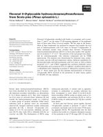
The bias of the fixed part of the diameter growth model was
examined by plotting the residuals as a function of the pre-
dicted variable and predictors of the model (figure 1). The
residuals of the fixed model part are correlated within each
Psurvive()
lkjt
1
1
b
0
b

1
BAL
lkjt
b
2
dbh
lkjt
T
lkt

´
+´+
èø
æö
–
èø
æö
exp+
e
lkjt
+=
Psurvive
()
lkjt
1
1
b
0
b
1

BAL
lkjt
b
2
id5
lkjt
´+´+()–()exp+
e
lkjt
+=
bias
y
i
y
ˆ
i
–()
å
n
=
bias%100
y
i
y
ˆ
i
–()n¤
å
y
ˆ

i
n¤
å

´=
RMSE
y
i
y
ˆ
i
–()
å
2
n 1–
=
RMSE%100
y
i
y
ˆ
i
–()
å
2
n 1–()¤
yˆ
i
n¤
å

´=
y
ˆ
i
Table II. Estimates of the parameters and variance components of
the diameter growth model (Eq. (1)), height model (Eq. (2)) and self-
thinning model (Eq. (3)).
Parameter Diameter growth
model (Eq. 1)
Height model
(Eq. 2)
Self-thinning
model (Eq. 3)
b
0
b
1
b
2
b
3
b
4
b
5
b
6
R
2
4.1786

–0.0070
–8.0476
0.6945
–0.0042
–1.1092
0.0764
0.0206
0.0821
0.3373
0.2400
0.5546
–0.3317
–0.0015
-
-
-
-
-
-
1.4553
0.8900
5.2060
–1.8150
0.0212
-
-
-
-
-
-

0.0030
0.9700
s
pl
2
s
tr
2
s
e
2
Individual-tree models for Scots pine 5
plot and tree (part of the residual variation is explained by ran-
dom plot and tree factor). This should be taken into account
when analysing figure 1. However, no obvious dependencies
or patterns that indicate systematic trends between the residu-
als and the independent variable can be found. The bias
showed a positive trend only when the predicted diameter
growth exceeded 2 cm per 5-year-period (figure 1), but diam-
eter growth greater than 2 cm is very rare. The relative RMSE
value for the diameter growth model was 64.1%.
The estimated height model describes tree height as a func-
tion of diameter at breast height, age, dominant height and
dominant diameter (Eq. (2)). Due to the form of equation (2),
the height of a tree with dominant diameter is equal to the
dominant height of the stand. Furthermore, when the age of the
stand increases the height differences between dominant trees
and the other trees in the stand are less pronounced. The esti-
mated height model had a R
2

value of 0.89. The relative bias
for the height model was 0.10% and the RMSE was 8.29%
(table III). There were no obvious trends in the bias of the
height model (figure 2).
3.2. Mortality models
The self-thinning model describes the relationship between
the square mean diameter and number of trees per hectare in a
stand (Eq. (3)). The R
2
value was 0.97, with an RMSE of 0.003
(table III). According to the model, the better the site the
higher the stocking level of the stand with differences between
sites being more pronounced in young stands (figure 3). The
relative bias and RMSE value for the self-thinning model were
0.23 and 17%, respectively. Owing to the logarithmic transfor-
mation of the predicted variable, a correction factor
should be added to the constant of equation (3).
The probability of a tree in P. sylvestris stands to survive the
next 5 years was estimated by two different models (Eqs. (4)
Table III. Absolute and relative biases and RMSEs of the diameter
growth model (Eq. (1)), height model (Eq. (2)) and self-thinning
model (Eq. (3)).
Criteria Diameter growth
model (Eq. 1)
Height model
(Eq. 2)
Self-thinning
model (Eq. 3)
Bias
Bias %

RMSE
RMSE %
0.0124 cm 5yr
–1
1.2
0.6600 cm 5yr
–1
64.1
0.0153 m
0.10
1.2000 m
8.29
4.30 trees ha
–1
0.23
325 trees ha
–1

17.00
Figure 1. Mean residuals (bias) of the diameter growth model as a function of stand age, basal area, site index, competition index (BAL),
predicted diameter growth and tree diameter.
s
st
2
2¤
6 M. Palahí et al.
and (5)) for two different situations. Equation 5 is used when
information on the past 5-year diameter growth of the subject
tree is available. Equation 4 is used when only average diam-
eter growth is available for the subject tree. The probability of

a tree surviving is best explained by its past diameter growth
and its competition index (Eqs. (4) and (5), table IV). The
Wald tests show that the parameter estimates of equations (4)
and (5) are significant (P < 0.05) (table IV). By analysing
equations (4) and (5) it can be deduced that the more sup-
pressed the tree is (the greater the competition index), the
smaller is the survival probability. The greater is the past
diameter growth (average growth or past 5 years growth), the
Table IV. Estimated parameters, their standard errors (S.E.), statistical significance and odds ratios for the logistic mortality models
(Eqs. (4) and (5))
a
.
Parameter Estimate S.E Wald statistics Significance Odds ratio (exp(b))
Mortality model 1 (Eq. 4)
b
0
b
1

b
2

c
2
-value
3.954
–0.035
2.297
94.039
0.286

0.005
0.613
190.821
43.788
14.021
0.000
0.000
0.000
-
0.965
9.943
Mortality model 2 (Eq. 5)
b
0
b
1
b
2
c
2
-value
2.938
–0.020
2.719
620.180
0.175
0.005
0.139
280.530
15.010

382.350
0.000
0.000
0.000
-
0.980
15.160
a
c
2
: Chi-square value.
Figure 2. Mean residuals (bias) of the height model as a function of stand age, dominant height, dominant diameter, tree diameter and predicted
tree height.
Individual-tree models for Scots pine 7
greater is the probability of a tree surviving. The probability
ratios of the covariates show that the past growth (Eq. (4)) and
5-year diameter growth (Eq. (5)) have the strongest relative
effect on the probability of a tree surviving. With continuous
variables, the probability ratio describes the change of proba-
bility per one unit change of covariate. This means for instance
that the probability of survival becomes 15 times higher
(Eq. (5)) with 1 cm increase in the past 5-year diameter
growth.
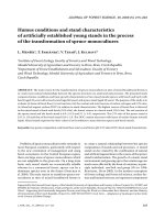
3.3. Simulation results
Figure 4 shows examples of actual and simulated stand
development for four stands with site indices 26, 19, 14 and
15 m at 100 years, respectively. The four selected plots cover
the range of variation in site index and stand age among the
plots used to develop the growth and mortality models.
Figure 4 shows that the model set developed in this study ena-

bles a very accurate long-term simulation of stand develop-
ment for the four selected stands.
Figure 5 shows the measured and predicted changes of dif-
ferent stand variables for all plots in all the measurements. It
is evident from these figures that there is no bias in the predic-
tions by the model set. However, the predicted range of varia-
tion in the 5-year change in basal area, mean diameter and
mean height is smaller than the observed change. This is
mainly due to the fact that the diameter growth model explains
Figure 3. Actual and predicted maximum number
of living trees per hectare as a function of mean
square diameter (D) estimated using the self-
thinning model (Eq. (3)). Each curve indicates the
self-thinning limit for a different site. The points
from the same plot are joined. Plots from the same
site class have the same symbol.
Figure 4. Measured and simulated stand development in four sample plots with site indexes 14, 15, 19 and 26 m at 100 years. The solid line
is the measured development and the dashed line is the simulated development. N is number of trees per hectare; G is basal area; H
g
is basal-
area-weighted mean height and D
g
is basal-area-weighted mean diameter.
8 M. Palahí et al.
only part of the variation in diameter increment. It should also
be noticed that the growth was simulated by using only the
fixed part of equation (1).
4. DISCUSSION
This study presented individual-tree models for P. sylves-
tris stands in north-east Spain based on permanent sample

plots measured an average of 5 times and ranging in site index
from 14 to 26 m at 100 years. In fitting the models, both meas-
ured dominant height and site index were used as predictors.
The site index model developed by Palahí et al. [19] can be
used to obtain dominant height when applying the models in
simulations. To predict mortality below the self-thinning limit,
the logistic survival functions may be used. When the self-
thinning limit is reached the logistic mortality functions may
be used to select the dead trees (those trees with the lowest sur-
vival probability).
In this study the slope (–1.815) of the self-thinning line is
different from the one given by Reineke [23] (–1.605), but it
is very similar to the slope obtained for Scots pine by Rojo and
Montero [26] in the Sistema Central (–1.836) and by Rio et al.
[25] for stands in the Sistema Ibérico and Central (–1.829) in
Spain. Hynynen [11] obtained for Scots pine in Finland a slope
equal to –1.844. This reflects a rather constant value for this
species in spite of changing environmental conditions.
According to this study, the intercept of the self-thinning line
was found to vary according to site index. This is in accord-
ance with the results obtained by Hynynen [11] for Scots pine
in Finland.
The data set in this study had limitations, which caused
problems in the modelling work and that can affect the model
predictions. The total number of plots available was only 24.
However, a good feature of the data was that the development
of plots was observed for a long time, up to 36 years. The data
did not have a representation of very young stands (under
33 years) and there was not much data from stands beyond the
normal rotation age (only 3 plots were measured at ages older

than 100 years). In addition, human errors associated with
diameter measurements were common. The breast height
diameter may not have been measured at exactly the same
height, and the direction of the diameter measurement may
have been different. This resulted in low precision of the diameter
Figure 5. Measured and predicted 5-year changes of all plots for all measurement intervals. N is number of trees per hectare; G is basal area;
H
g
is basal-area-weighted mean height and D
g
is basal-area-weighted mean diameter.
Individual-tree models for Scots pine 9
increment observations, which are differences of two succes-
sive dbh measurements. This is reflected in the value of the
coefficient of determination (0.24). The precision of the diam-
eter growth predictions, therefore, needs to be viewed within
the data constraints exposed above.
Height growth models could not be developed because
there were not enough sample tree heights per plot measured
more than once. The height model developed in this study is
useful for predicting tree heights, for instance in inventory sit-
uations when the dominant height and tree diameters are
measured, but all trees are not measured by height. The model
predicts tree height accurately and, therefore, it can be used for
growth simulation as well.
Examples of simulated stand development were used to
demonstrate how the equations work together in long-term
simulations. Simulation results were presented for four stands,
which represent the range in site index (from 14 to 26 m at 100
years) of the data set. The system of equations developed in

this study appeared to provide accurate predictions of stand
development (figure 4). Therefore, the tree-level models
reported in this study could confidently be used to predict the
growth of different P. sylvestris stands on several sites in
Spain.
This study is the first, known by the authors, on individual-
tree growth models for Scots pine in Spain. Scots pine in Spain
is a species of great economic, ecological and social impor-
tance and the models presented in this study can provide
valuable information for further studies on optimising the
management and evaluating alternative management regimes
for the species.
Acknowledgments: Financial support for this project was given
by the Forest Technology Centre of Catalonia (Solsona, Spain). We
gratefully acknowledge the data provided by the Instituto Nacional de
Investigaciones Agrarias (Spain). We thank Mr. Tim Green for the
linguistic revision of the manuscript and Jo Van Brusselen and an
anonymous reviewer for the French translation of the abstract.
REFERENCES
[1] Alder D., A distance-independent tree model for exotic conifer
plantations in East Africa, For. Sci. 25 (1979) 59–71.
[2] Avila O.B., Burkhart H.E., Modeling survival of loblolly pine trees
in thinned and unthinned plantations, Can. J. For. Res. 22 (1992)
1878–1882.
[3] Bredenkamp B.V., Burkhart H.E., An examination of spacing
indices for Eucalyptus grandis, Can. J. For. Res. 20 (1990)
1909–1916.
[4] Cao Q.V., Prediction of annual diameter growth and survival for
individual trees from periodic measurements, For. Sci. 46 (1)
(2000) 127–131.

[5] Clutter J.L., Forston J.C., Piennar L.V., Brister G.H., Bailey R.L.,
Timber management – a quantitative approach, Wiley, New York,
1983.
[6] Drew T.J., Flewelling J.W., Some recent Japanese theories of yield
density relationships and their application to Monterey pine
plantations, For. Sci. 23 (1977) 517–534.
[7] Eerikäinen K., Predicting the height-diameter pattern of planted
Pinus kesiya stands in Zambia and Zimbabwe, For. Ecol. Manage.
(in press).
[8] Gadow K., Hui G., Modeling forest development, Faculty of Forest
and Wodland Ecology, University of Göttingen, 1998.
[9] González S.C., Bravo F., Density and population structure of the
natural regeneration of Scots pine (Pinus sylvestris L.) in the High
Ebro Basin (northern Spain), Ann. For. Sci. 58 (2001) 277–288.
[10] Hamilton D.A., Extending the range of applicability of an
individual tree mortality model, Can. J. For. Res. 20 (1990)
1212–1218.
[11] Hynynen J., Self-thinning models for even-aged stands of Pinus
sylvestris, Picea abies and Betula pendula, Scand. J. For. Res. 8
(1993) 326–336.
[12] Hynynen J., Predicting the growth response to thinning for Scots
pine stands using individual-tree growth models, Silva Fennica 29
(1995) 225–246.
[13] Lonsdale W.M., The self-thinning rule: dead or alive?, Ecology 71
(1990) 1373–1388.
[14] Lowell K.E., Mitchel R.J., Stand growth projections: Simultaneous
estimation of growth and mortality using a single probabilistic
function, Can. J. For. Res. 17 (1987) 1466–1470.
[15] Mabvurira D., Miina J., Individual-tree growth and mortality
models for Eucalyptus grandis (Hill) Maiden plantations in

Zimbabwe, For. Ecol. Manage. 161 (2002) 231–245.
[16] Monserud R.A., Simulation of forest tree mortality, For. Sci. 22
(1976) 438–444.
[17] Montero G., Cañellas I., Ortega C., Del Rio M., Results from a
thinning experiment in a Scots pine (Pinus sylvestris L.) natural
regeneration stand in the Sistema Ibérico Mountain Range (Spain),
For. Ecol. Manage. 145 (2001) 151–161.
[18] Munro D., Forest growth models – a prognosis, in: Fries J. (Ed.),
Growth models for tree and stand simulation, Proceedings of the
IUFRO working party S4.01-4, 1974, pp. 7–21.
[19] Palahí M., Tomé M., Pukkala T., Trasobares A., Montero G., Site
index model for Pinus sylvestris in north-east Spain, Manuscript
(2003).
[20] Pukkala T., Studies on the effect of spatial distribution of trees on
the diameter growth of Scots pine, Publications in Science No. 13.
University of Joensuu, 1988.
[21] Pukkala T., Predicting diameter growth in an even-aged Scots pine
stand with a spatial and non spatial model, Silva Fennica 23
(1989)101–116.
[22] Rautiainen O., Spatial yield model for Shorea robusta in Nepal,
For. Ecol. Manage. 119 (1999) 151–162.
[23] Reineke L.H., Perfecting a stand-density index for even-aged
forests, J. Agric. Res. 46 (1933) 627-638.
[24] Rio M. del., Régimen de claras y modelo de producción para Pinus
sylvestris L. en los sitemas Central e Ibérico. Tesis Doctoral,
ETSIM-UPM, Unpublished, 1998, 219 p.
[25] Rio M. del., Montero G., Bravo F., Analysis of diameter-density
relationships and self-thinning in non-thinned even-aged Scots pine
stands, For. Ecol. Manage. 142 (2001) 79–87.
[26] Rojo A., Montero G., El pino silvestre en la Sierra de Guadarrama,

Centro de publicaciones del Ministerio de Agricultura, Pesca y
Alimentación, 1996, 293 p.
[27] SAS Institute Inc., SAS/STAT
®
User’s guide, version 8, Cary, NC,
SAS Institute Inc., 1999, 3884 p.
[28] Shafii B., Moore J.A., Newberry J.D., Individual-tree diameter
growth models for quantifying within stand response to nitrogen
fertilisation, Can. J. For. Res. 20 (1990) 1149–1155.
[29] SPSS Inc., SPSS Base system syntax reference Guide. Release 9.0,
1999.
[30] Soares P., Tomé M., Skovsgaard J.P., Vanclay J.K., Evaluating a
growth model for forest management using continuous forest
inventory data, For. Ecol. Manage. 71 (1995) 251–265.
[31] Tennent R.B., Individual-tree growth model for Pinus radiata,
N. Z. J. For. Sci. 12 (1982) 62–70.
10 M. Palahí et al.
[32] Vanclay J.K., Compatible deterministic and stochastic predictions
by probabilistic modeling of individual trees, For. Sci. 37 (1991)
1656–1663.
[33] Vanclay J.K., Modelling forest growth and yield: Applications to
mixed tropical forests, CABI Publishing, Walingford, UK, 1994.
[34] Yoda K., Kira T., Ogawa H., Hozumi K., Self-thinning in
overcrowded pure stands under cultivated and natural conditions,
J. Biol. Osaka City Univ. 14 (1963) 107–129.
[35] Zeide B., Tolerance and self-tolerance of trees, For. Ecol. Manage.
13 (1985) 149–166.
[36] Zeide B., Analysis of the 3/2 power law of self-thinning, For. Sci.
33 (1987) 517–537.
[37] Zhang S., Amateis R.L., Burkhart H.E., Constraining individual

tree diameter increment and survival models for Loblolly pine
plantations, For. Sci. 43 (1997) 414–423.
To access this journal online:
www.edpsciences.org