Báo cáo lâm nghiệp:"Shoot growth and phenology modelling of grafted Stone pine (Pinus pinea L.) in Inner Spain" potx

527
Ann. For. Sci. 60 (2003) 527–537
© INRA, EDP Sciences, 2003
DOI: 10.1051/forest:2003046
Original article
Shoot growth and phenology modelling of grafted Stone pine
(Pinus pinea L.) in Inner Spain
Sven MUTKE, Javier GORDO, José CLIMENT, Luis GIL*
U.D. Anatomía, Fisiología y Genética Forestal, ETS Ingenieros de Montes, Universidad Politécnica de Madrid,
Ciudad Universitaria s/n, 28040 Madrid, Spain
(Received 26 April 2002; accepted 13 November 2002)
Abstract – Shoot elongation, flowering phenology, branch thickening, needle and cone growth was monitored during four years in grafted stone
pines in Inner Spain. The relevance of environmental influence on growth and flower regulation in Mediterranean stone pine as nut crop is
stressed. Different models of thermal time compute were compared for characterizing phenostage onset, shoot and cone growth response to
temperature. Non-linear regression models for relative length of preformed shoots and relative cone diameter were fitted in thermal-time scale.
Shoot-growth timing was characterized by a common degree-day sum between years. Correlation of June rainfall with shoot length and flower
bearing in the next year and with current needle and branch diameter growth was highly significant. Also, summer shoots and a second female
flowering occurred occasionally in leader branches in dependence on June rainfall, but cone-setting failed due to the absence of pollen.
Phenological model of the variation between years were consistent with observations in mature non-grafted stone pines.
stone pine (Pinus pinea) / growth and flowering phenology / phenology modelling / growing-degree-days
Résumé – Modélisation de la croissance des pousses et de la phénologie du Pin pignon greffé (Pinus pinea L.) en Espagne Centrale.
L’allongement des pousses, la phénologie de la floraison, l’épaississement des branches et le développement des aiguilles et des cônes ont été
suivis pendant quatre ans chez des pins pignon greffés dans une plantation située en Espagne centrale. L’influence des conditions
environnementales sur la croissance et la régulation de la floraison est étudiée sur le Pin pignon méditerranéen en tant que producteur de graines.
Différents modèles basés sur les sommes des températures (degrés jours) ont été comparés afin de caractériser les stades phénologiques et
l’influence de la température sur la croissance des pousses et des cônes. Des modèles de régression non-linéaire ont pu être estimés reliant la
longueur relative de la pousse préformée et le diamètre relatif des cônes avec l’échelle de temps thermique. La courbe de croissance des pousses
est caractérisée par une même somme de degrés-jour chaque année. Une corrélation significative est établie la pluviométrie du mois de juin et
la croissance des aiguilles et la croissance entre épaisseur des branches de l’année courante ou avec la longueur des pousses et la floraison portée
l’année suivante. La mise en place d’une pousse estivale et d’une seconde floraison femelle peuvent se produire occasionnellement sur les
branches maîtresses en relation avec les précipitations du mois de juin, cependant les cônes ne subissent aucune maturation en raison de

l’absence de pollen. Des modèles phénologiques de la variation entre années concorde avec des observations réalisées sur des Pins pignons
matures non greffés.
pin pignon (Pinus pinea L.) / phénologie de la croissance et de la floraison / modélisation de la phénologie / sommes des températures
1. INTRODUCTION
In the last decade, modelling of tree phenology has gained
new attention in forest science, due to the discussion about the
impact of climatic change on tree growth and forest ecosys-
tems functioning and stability [25, 27]. Moreover, emerging
functional-structural growth modelling needs a deeper view in
environment-plant interaction to gain accuracy [31, 33].
Whereas traditional forest modelling methods analysed stand
growth and structure using mass variables, some more recent
methods for individual tree-growth models explore a more
detailed representation based on the plant-architecture para-
digm [6, 30, 44]. This approach focuses on inherent, geneti-
cally determined topology and on quantitative laws of tree
geometry [4, 42]. To achieve environment sensibility, external
influences, e.g. the relationship between annual climate
parameters and growth must be taken into account [5, 47].
Air temperature is recognized as the main environment fac-
tor regulating phenological timing and growth rates in temper-
ate plants [7, 15, 47]. Phenology dependence on temperature is
related both to the amount of chilling units for budburst and to
the temperature-dependent acceleration of biological proc-
esses [3, 24]. Already De Candolle quantified in 1855 this
effect through the concept of thermal integral, a time-tempera-
ture product above a certain value t
0
[9]. This threshold value
has been shown to vary among species and provenances [3].

* Corresponding author:
528 S. Mutke et al.
The relevance of temperature as a regulation factor of tree phe-
nology in cold and temperate regions has been studied by
numerous authors [13, 25], but this relationship is less known
for Mediterranean forest species. There, water availability has
been usually regarded as the main environmental factor,
affecting growth amount rather than the timing of phenologi-
cal events [27]. Thus, the dependence of plant phenology on
temperature still must be studied also in the Mediterranean
region, in order to establish accurate models [18].
Stone pine is one of the most characteristic trees of the
Mediterranean flora, adapted to dry sandy or rocky soils where
it forms open stands, pure or mixed with maritime pine (Pinus
pinaster Ait.), some species of Juniperus or Quercus and other
understorey species. Like other temperate pines, stone pine
has a monopodial, cyclic growth pattern. Annual shoots, pre-
formed in buds on the apex of last year’s shoots, bear a subap-
ical whorl of lateral buds and female strobili [32]. In stone
pine, shoot elongation occurs mainly in spring; polycyclic
growth is rare in grown-up trees and if present, the second
growth unit is always quite shorter than the first one. Occa-
sionally, summer shoots may bear a second female flowering.
An outstanding trait of stone pine are the large cones (8–14 to
7–10 cm) with edible seeds (15–20 mm) that need three years
to ripen. In consequence, cones of three consecutive crops
coincide in the tree each spring, when the new strobili are
induced. Because of the commercial use of the edible kernels,
cones are the main yield of the stonepine forests, with higher
income for forest owners than timber. Actually, current breed-

ing and improvement programs aim to the potential use of
grafted stone pine as an alternative crop in specific plantations
for cone yield in farmlands, but further experimentation about
management techniques is still required [11, 38, 39]. Annual
cone production (200–600 kg per hectare) means a biomass
allocation similar to bole volume growth, which is less than
1m
3
/ha in common stonepine forests, stocking poor, exces-
sive draining soils. Hence, reproductive structures must be
taken into account in any functional-structural growth model.
Additionally, physiological stress due to the xeric growth con-
ditions may sharpen growth response to environment factors,
as observed in other pine species [41]. E.g., stone pine has a
strong masting habit like many Mediterranean species and
yearly income from pine forests varies widely. The very irreg-
ular fruitfulness has been related to climate factors and nega-
tive autocorrelations with previous crops [20]. Thus, yield
modelling with a non-sensitive approach would fail to inte-
grate these sources of between-years variance with great bio-
logical and economic importance. On the other hand, there is
no published information about the phenology of inland stone-
pine.
Most temperature-based phenological models published for
forest species concern two singular ontogenetic events: the
onset of budburst in cold and temperate climates [24, 25, 47]
and the flowering, especially in seed orchards [13, 15, 35].
Fewer studies have been published about shoot growth as
another aspect of ontogenetic development linked to spring
temperature in pines [2, 14, 23]. Shoot elongation is not a dis-

crete event but a continuous process observed by repeated
measurements. Moreover, Mediterranean pines like Pinus
pinea do not have well defined smooth winter buds, nor a clear
budburst, but the stem units of their long buds “just start elon-
gating” [14]. Phenological parameters are thus best derived
from growth curves rather than assessed visually as discrete
phenostages.
Temperature relevance for leaf expansion rate has been
stressed in non-woody species at organ, tissue and cell level
[22]. In roots and monocot leaves, processes involved in
growth show a linear response to thermal integral because one
clearly defined meristematic zone produces continuously and
at constant rate new cells which subsequently elongate,
whereas leaf growth in dicot species like sunflowers occurs in
whole the leaf area, thus not absolute, but relative growth rate
related to current size is constant in thermal time [21]. Both in
monocot and dicot leaf growth, cell division and cell elonga-
tion are nearby in time and space. Sequence is quite different
in preformed shoot growth of woody axes, like those in pines:
in temperate climates, differentiation (activity of apical meris-
tem) takes place during bud formation the year before and only
in following spring this preformed winter bud breaks dor-
mancy and elongate (subapical growth) [10, 32]. The final
length of pine shoots is determined mainly by the number of
stem units and less by their mean length [23, 28, 29]. On the
other hand, as shoot elongation consists in the expansion of
stem units (vacuole expansion) and does not depend on meris-
tematic activity [29], growth rate is not limited by the maxi-
mum cell division rate as leaf expansion is [22], but will be
determined by the expansion rate of the individual stem unit

and by the simultaneous or sequential elongation of these
units. By the same reasons, the response to temperature may
not be linear but sigmoid in time [14, 26]. It may be expressed
as relative growth referred to final length, in order to compare
shoots with different final length (numbers of stem units).
In opposition to annual plants, detailed measurements of
shoot elongation or actual temperature at individual organ
level are not easy to perform in crowns of mature trees. In
addition, detailed growth chamber or greenhouse experiments
are normally limited by tree size and age; so most experiences
have been performed on seedlings or saplings with immature
growth habit [22, 23]. In this context, the study on low grafted
trees offers the possibility to observe mature shoot growth in
field on an intermediate scale between physiological moni-
tored samples in controlled environment and real growth condi-
tions in forest stands. The main objective of the present paper
is to study the timing and climate influence on shoot and nee-
dle growth, flowering and cone development of stone pine in
a sample of grafted trees. Especially the response functions
that link shoot elongation and cone growth to thermal time are
analysed, in order to evaluate if the relation between growth
rate and thermal time can explain differences in phenology
between years.
2. MATERIALS AND METHODS
2.1. Site description and plant material
Field data were measured in the Meseta Norte provenance region
(central Douro Basin). This sedimentary plateau at 600–900 m a.s.l.
is the coldest and one of the driest areas of natural stonepine distribu-
tion. Actually, Inner Spain is the only native stonepine area far
from coastline. Its climate is not genuine Mediterranean, but has a

Growth and phenology modelling of Stone pine 529
continental tendency with hot, dry summers and long, harsh winters.
Average temperatures range from 10.1 to 13.5 ºC and occasional late
frosts occur up until May or June and early frosts from September or
October. Yearly rainfall ranges from 350 to 600 mm with a very
irregular distribution as much between years as between seasons [43].
The plant material for this study consisted of homoplastic grafted
stone pines in a clone bank, located at 4° 20' W, 41° 35' N and
890 m a.s.l. in Quintanilla, province of Valladolid. Average temper-
ature is 10.1 °C and rainfall reaches 447 mm. Scions came from high
cone-yield plus trees, mass-selected within the Meseta Norte stone-
pine stands. The ramets were planted in 1992 in 6 × 6 m setting in a
gap of an aged stonepine stand, so lateral pollination guarantees cone
setting. An automatic weather station within the clone bank records
daily maximum and minimum temperature and rainfall. The planta-
tion is not watered.
2.2. Experimental design
The sampling design was hierarchical, marking three grafts of
each of the three most cone-bearing clones of the plantation and three
branches in each of these nine ramets. During four years (1997–
2000), shoot elongation and diameter growth of branches and three-
year cones were monitored, and flowering was followed in these
27 apices. Shoot and cone measurements were taken once or twice a
week during the main growing period in spring and once a month in
the rest of the growing season, except in 1998, with lower measuring
frequencies. Total annual shoot growth was partitioned into spring
shoot and terminal bud/summer shoot. Branch diameter d
B
was meas-
ured monthly at the base of last year’s shoot. Pearson’s product-

moment correlations were used to estimate relationships between
spring-shoot growth parameters. Needle growth was measured in 1997
and 2000, while in the other two years only final needle length was
computed. The influence of rainfall on shoot and needle length and
cone diameter was studied by regression analysis. Average final values
in the four years were regressed against rainfall amount for each period
of one, two or three successive months between January and August.
Phenology of shoot and flower strobili development was assessed
after a categorical scale from stage A (close winter bud) to stage G
(formation of new terminal bud). Analyses focused on the three most
relevant to female flowering:
Stage D: on the shoot tip, strobili elongate still covered with bud
scales.
Stage F: the ovuliferous scales are separated to allow the pollen
grains to reach the micropyles and pollinate the ovules.
Stage G: the pollinated strobili close by swelling their scales. The
vegetative shoot tip has finished its elongation and a
whorl of long shoot buds is formed and topped by the
new terminal bud.
Female flowering phenology was monitored counting strobili per
shoot in each stage. Male flowering did not occur in the studied
grafts.
Characteristic dates corresponding to fixed percentages of spring
shoot and cone growth were interpolated between consecutive meas-
urements. These dates were T
0.1
, T
0.5
and T
0.9

, corresponding to 10%,
50% and 90% of the total growth. Average daily growth rate (ADG)
between T
0.1
and T
0.9
was calculated for each shoot and cone. The
branch-diameter data were too rare to estimate characteristic dates.
The relationship between heat sums and growth for each year was
examined graphically before a non-linear regression model was fitted
for spring shoot length at moment t with thermal time; cone growth
was modelled by analogous methods, though following methodology
refers only to shoots. Due to a late frost in early May 1997 that pre-
sumably damaged some shoots tip; in this year, data of six shoots and
two cones with erratic growth curves after this extreme meteorologi-
cal event were excluded from analysis.
During the elongation phase, the current length of each spring
shoot may be expressed by the relative or standardized growth
referred to final elongation, discounting the initial bud length:
(1)
where d: date [Julian days]; L
0
: winter bud length; L(d): shoot length
at d; L: inal spring shoot length; G(d): accumulative form of distribu-
tion function with G(–∞) = 0, G(∞)=1.
Winter bud length L
0
and final length L of each shoot were actual
measured data; hence fitting consisted in adjusting a growth function
G(dd) between 0 and 1. Chilling request for budburst was not consid-

ered in the present study, since about 1000 hours below 7 ºC occur
from September until January and 2000 until March in the study area.
Chilling was thus assumed widely enough for breaking bud dormancy.
As discussed before, the growth-rate dependence on temperature
may be expressed rather by the use of thermal time than by calendar
time as argument of function G. This variable can be computed by the
De Candolle’s definition of degree-days sum dd as a rectangular daily
approximation to the double integral of temperature curve t(T) above
threshold t
0
in time interval [T1; T2]:
d tdT
when t>t
0
, null else. Referred only to the temperature axis, this
response is a broken-line curve, constantly null below t
0
and linearly
increasing with temperature above t
0
. This definition should be com-
pleted by an upper threshold, when temperature reaches its optimum
and growth rate is constant in spite of further increments of t (or even
may decrease due to metabolism costs). This upper threshold is situ-
ated in species of temperate climate zones normally about 25–28 ºC
[3, 22]. The resulting constant/linear/constant broken line model of
biological relevance of environment temperature can be substituted
by a differentiable sigmoid curve, as is Sarvas’ forcing unit function
FU(t) (Eq. (2)) [15, 24]. The growth response between FU = 0 (no
response) to FU = 1 (maximum growth rate) to daily temperature

average t is formalized adjusting parameter w after subtracting char-
acteristic temperature t’ for which response reach half of its maxi-
mum [14, 24]:
(2)
where t
d
: daily mean temperature at day d [ºC]; t’: characteristic tem-
perature (inflexion point) [ºC]; w: slope parameter [ºC
–1
].
The FU distribution may be combined with an exponential growth
curve in the so calculated FU scale, adjusting this set of two equa-
tions. But whereas simple exponential function is symmetrical to
inflection point t’, the observed growth pattern in stone pine was quite
left skewed in both time and thermal-time scales. In those cases, rec-
ommended functions are double exponentials like Gumbel or Gom-
pertz, which are not symmetrical in the point of inflection [19]. Since
growth asymptote is standardized to the unity, a modified function
with two parameters b (location) and c (slope) was used. Parameter c
was negative, so the function that fulfils the limit conditions of equa-
tion (1) is:
(3)
where Σhu: daily approximation to thermal integral from starting day
d
0
to date d; b: moment of maximum growth (inflexion point of
cumulative distribution); c: slope parameter.
For comparison of both methods, the model was fitted for forcing-
units sum and also for degree-days sum as argument of G, the latter
L

d() L
0
LL
0
–()Gd()×+=
1
t
0
tT()
∫
T
1
T
2
∫
F
Ut
d
()
1
1 e
wt
d
t
′
–()
+
=
Ghu
d

0
d
∑




1 e
e
Σhu b–()–
c

–
–=
530 S. Mutke et al.
computed by a triangular approximation of daily thermal integral
(Tab. I). Calculating the thermal-time sum uses daily maximum and
minimum temperature during five or six months, so parameter calibra-
tion of the model formed by the set of two equations (heat unit amount
in time and non-linear growth response to it) can not be solved using
any standard mathematical optimisation procedure. Hence, model cal-
ibration was done by heuristic search comparing output of re-parame-
terized thermal-time model, in order to assign values to the unknown
model parameters so as to maximize the models fit to data by minimiz-
ing the residual variance [40], estimated by the coefficient of variance
of location parameter b between years. As thermometric input was
computed with 1 ºC precision, parameters of the heat-sum functions
were calibrated also to integers (except w with 0.05 precision). In addi-
tion, this technique allows analysing the sensitivity of the response
model to changes in input parameters and thus estimating its robust-

ness. In Inner Spain, the conventional starting date d
0
for thermal inte-
gral computing in horticultural phenology studies is February first (day
32 of Julian Calendar). In the studied region, this is quite earlier than
visible shoot-growth initiation in stone pine, though in this month root
activity recovers and it is in mid-February when resin flow starts to
cover pruning wounds [37]. But as in some studies in temperate climate
zones heat sum was computed from January First, these two alternative
starting dates and various values for characteristic temperature t’ (10,
12, 13, 14, 16 ºC) and slope parameter w (–0.20, –0.25, –0.30,
–0.35 ºC
–1
) were used to calculate different FU amounts correspond-
ing to each sample date, as well as amounts of degree-days for various
threshold temperatures t
0
(0, 1, 2, 3, 4, 5, 8, 12 ºC) with fixed superior
threshold 25 ºC. Since the registered daily mean temperatures in the
four springs were normally below 20 ºC and never exceeded 25 ºC,
degree-day model fitness was affected mainly by the lower threshold,
whereas accuracy of (here fixed) upper threshold estimation was sec-
ondary.
With the data of each individual spring shoot and cone growth,
growth parameters b and c were estimated for each of these alterna-
tive thermal-time approximations as independent variable, using the
DUD non-linear regression method of iterative NLIN procedure in
SAS

system [46]. Fitting each individual growth curve independ-

ently to thermal time allows obtaining individual growth parameters,
in order to detect outliers previously to mingling the data in means
and to study parameter distribution, correlations and differences
among groups. Moreover, the inherent non-linearity of metabolic
processes warns against using averages, because the non-linear func-
tion of the mean is seldom identical to the mean of the non-linear
functions and may lead to bias [47]. Residual minimization of indi-
vidual non-linear regression was not a valid criterion for model selec-
tion, as the consecutively measured values of the same shoot are not
independent data. Moreover, most cases presented R
2
above 0.95 or
yet 0.99 (analogous to the linear case, R
2
was computed as 1 – SSE/
CSS, where SSE is the error sum of squares obtained from non-linear
regression and CSS is the corrected total sum of squares for the depend-
ent variable). So model calibration methodology consisted in three
steps: (1) perform non-linear regressions for each shoot/cone growth
against each thermal-integral function; (2) evaluate accuracy of these
regressions by residual analysis and (3) study the distributions of
parameter values in dependence on thermal-integral model and param-
eters and select best model and parameterization.
In the next step, analysis of variance for parameter b and c values
were performed with clone and year as fixed effects and metric shoot/
cone variables (final length/diameter, branch diameter, number of
cones, number of flowers) by GLM procedure in SAS

[46]. Fulfill-
ing of ANOVA assumptions, especially the homogeneity of residual

variances, was checked by graphic residual analysis. After checking
normality of individual parameter values, great means were estimated
as 95%-confidence interval of means ± 1.96 standard deviation
between years.
3. RESULTS
3.1. Environment influences on shoot, needle and cone
growth
Spring shoot elongation took place mainly from April to
June (Fig. 1). Shoot growth was acropetal with a low growth
rate in early spring and its maximum at the end of May close
to the elongation stop, resulting in a left-skewed curve. In the
unusually warm spring of 1997, shoot phenology was antici-
pated by several weeks in comparison with the other years
(Figs. 1 and 2); but a night frost in May 8 damaged soft tissues
of some shoot (data of six shoots were excluded from results
Table I. Formulae of triangular approximation to the temperature
curve in one day. M: maximum temperature; m: minimum
temperature measured in the day; t
0
: inferior threshold temperature
of the model; t
s
: superior threshold temperature of the model [ºC].
(1) dd = 0 if m < M < t
0
< t
s
(2)
if m < t
0

< M < t
s
(3)
if t
0
< m < M < t
s
(4)
if t
0
< m < t
s
< M
(5) dd = t
s
– t
0
if t
0
< ts < m < M
dd
Mt
0
–()
2
2 Mm–()
=
dd
Mm+
2

t
0
–=
dd
M
2
m
2
Mt
s
–()
2
–+
2 Mm–()

t
0
–=
Figure 1. Average shoot elongation (  spring shoot;
- - - total annual growth) and cone growth (without
labels) of 27 sampled shoots in four years.
Growth and phenology modelling of Stone pine 531
nor are represented in the figures), and in the following cold,
rainy weeks shoot growth broke down. Numerous female
conelets necrotized also and aborted. On the contrary, late
frosts in the other measuring years had no influence on shoot
growth rate and produced no visible damage on shoots or
flower buds, less developed than in 1997. In 1999, low mid-
May temperatures reduced shoot elongation rate, too, but

growth recovered when temperatures rose (Fig. 2).
In the four measured years, June was the only period for
which rainfall was positively related with average final length
L of spring shoots of the next year (Fig. 3). This parameter
accounted for more than 99% of the variation of average
spring-shoot length between the four years. The rainfall of the
current growing season showed no influence on spring shoot
length, but June rain seemed to determine the presence of summer
shoots (lammas growth) in the same year (Fig. 3). These
proleptic shoots, either partially elongated or fully developed,
appeared in vigorous branches in 1997 and 1998, responding
to a June rainfall above 30 mm. Seven of the nine sampled
grafts expressed summer growth. A second female flowering
appeared in some of these summer shoots in July but strobili
aborted because of the lack of pollen. In fall, no shoot or cone
growth was observed. Average needle length and branch
diameter growth showed a direct relationship with current
June rainfall (Fig. 3), although with lower coefficients of
determination than those of next year’s shoot length. July or
August rainfall showed no effect on needle length and branch
thickening, though both grew until September. Needle growth
rate was nearly constant in time. The oldest (2 or 3 year old)
needle cohorts decayed and fell in June.
3.2. Phenology modelling
Growth pattern of occasional lammas shoots showed no
dependence on current temperature, temperature influence on
growth rate was thus modelled only for preformed spring
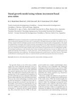
shoots and cones. In the graphic comparison of between-year
coefficient of variation of shoot growth parameters (Fig. 4),
only values near the optimum are represented. Ceteris paribus,

starting date February First performed always better than Jan-
uary First. Among the tested threshold temperatures, t
0
= 1ºC
showed the lowest coefficient of variation (1.13%) for average
location parameter b of shoot elongation. This value is quite
similar to the value 1.15% obtained for the forcing unit func-
tion when parameters are w=–0.2 ºC
–1
, t’ = 13 ºC (that is just
half the distance between best linear model’s thresholds 1º and
25 ºC). In fact, both curves are nearly proportional within the
range 5–21 ºC (Fig. 5) and gave thus nearly the same predic-
tion for growth curves in spring, when daily mean tempera-
tures rarely exceeded this values. Cone growth parameter b
had also low coefficient of variation between the three years
(1.47%) with t
0
= 1 ºC. Further results are thus shown for this
common threshold, although t
0
= 2ºC performed slightly bet-
ter for cone growth prediction (Cv 1.42%). Fitted individually
to thermal time above threshold 1 ºC, growth function (Eq. (3))
absorbed 99.38–99.998% (R
2
) of temporal variation of shoot
length and 99.61–99.94% for cone diameter even in atypical
spring 1997, though residuals evidenced certain lack of fitness
of the curves adjusted to cone growth (Figs. 7 and 8).

In the following (Tabs. II–IV), results are exposed only
referred to degree-days sum above 1 ºC, whereas redundant
references to FU model were omitted. The degree-day approach
was preferred for two reasons. (1) The inferior threshold tem-
perature of growth t
0
is a more intuitive concept than Sarvas’
characteristic temperature t’ and has a clearer biological inter-
pretation. (2) The degree-day sum models a local linear
dependence of biological processes on temperature below
upper threshold, without attempting to extrapolate for higher
temperatures, whereas the acceptation of the FU function,
though fitted mainly with data in its central nearly linear interval,
Figure 2. Current average shoot growth rate (—) of
27 sampled shoots and average temperature (- - -) in four
springs. Vertical scale: 1 unit = 2 mm/day; 1 unit = 5 ºC.

Figure 3. Tendencies of average shoot and needle length, branch
thickening and flower number in dependence on rainfall during June.
Left scale [mm]: a. spring shoot (next year); b. summer shoot; c.
needle. Right scale: d. diameter increment [mm]; e. flowers per apex
(next year).
532 S. Mutke et al.
would imply conceptually a consistent growth-rate increment
up to mean temperatures of 35 ºC (Fig. 5) that is biologically
fairly uncertain.
Shoot and cone growth phenology was quite similar in the
four years when expressed in thermal time (Fig. 6), except in
1997 when cold May reduced somewhat the anticipated flush-
ing. But even in this year, the rescaled shoot-growth curve is

smooth and lack the dramatic breakdown observed in time
scale (Fig. 1). Great mean values of the growth parameters
were b = 813 ± 18 dd and c = –170 ± 30 dd for spring shoots
(Tab. II). Analysis of variance showed no significant effect of
clone or year on shoot growth location parameter b, but both
factors as well as their interaction influenced significantly
slope parameter c (Tab. III). Parameter b depended also on
branch diameter, c on final shoot length, and parameters b and
c were significantly correlated. Cones presented a less pro-
nounced relative growth (c) and a later maximum (b) than
shoots, with average values b =1.094 ± 32 dd and c = –360 ±
73 dd. Actually, when shoot elongation was already finishing
(T
0.9
), cones reached just half their size (Tab. II). Cone growth
anticipated in early spring of 1997, though it was nearly linear
and coincident in the four years beyond 1000 degree days
(Fig. 6). Nevertheless, both cone growth parameter c and b
varied significantly between years and clones, also interac-
tions and correlation between b and c were present, whereas
final cone diameter did not influence the relative growth
parameters.
Monitoring phenology in thermal time reduced the range
between years for the moment of maximum shoot growth from
18 days in Julian time scale to 20 degree-days, which corre-
spond to the heat accumulated in less than two days, this is,
less than real sample frequency. For cone growth, these differ-
ences decreased from 13 days to 37 degree-days (less than
3 days) (Tab. II). The model parameterized with great mean
values of b and c achieved to predict at each sample date in the

four years current average spring-shoot length from degree-
days sum, winter-bud and final shoot length means with pre-
diction errors smaller than 25 mm; current average cone diameter
was predicted similarly with errors smaller than 10 mm (data
not included).
Total spring shoot elongation L was correlated with the
actual daily growth rate ADG of the shoot, but not with its
growth duration [dd
0.1
, dd
0.9
] (Tab. IV). The branch diameter
had a weak correlation with reproductive competence (NF, NC:
number of female flowers and cones) and a negative correla-
tion with the degree-day sums b, dd
0.1
, dd
0.5
and dd
0.9
, which
were correlated with each other. Slope parameter c was corre-
lated positively with growth rate ADG and growth onset dd
0.1
and negatively with growth finish dd
0.9
. Cone parameters b
and c were not correlated with parameters of bearing apex, but
they were correlated with each other.
3.3. Flower phenology

The onset of conelet phenostage showed a direct relation-
ship with the elongation of the bearing shoot (data not shown,
average values in Tab. II). Flower bud burst (stage D) took
place when half of the shoot growth had taken place and recep-
tivity (stage F) when shoot had nearly finished elongation. The
end of receptivity (stage G) occurred after shoot elongation
Figure 5. Best parameterisations of the two alternative thermal-
integral functions. Broken line model (degree days) and sigmoid
function (Forcing units).
Figure 4. Variability of Gompertz parameters b
and c for individual shoot elongation (a) and
cone growth (b) in dependence on thermal-time-
function parameters. Cv% Coefficients of varia-
tion between annual means in dependence on:
dd: degree-days sum above threshold tempera-
ture t
0
[ºC] from February First (ddf) or January
First (ddj) (lower axis); w / t’: FU function para-
meters [ºC
–1
/ ºC]: j: from January First, else
February First (upper axis).
Growth and phenology modelling of Stone pine 533
had ceased and had no apparent relationship with other shoot
events. The mean duration of stage F ranged from 12 to
21 days in the four sampling years (Tab. II). Variation in stage
onset was greater within than between trees or clones, so indi-
vidual antesis overlapped widely (data not included). In 1997,
stage D onset anticipated due to mild April weather, but cold

May conditions maintained flower phenology delayed at this
stage, beside frost damages already mentioned (Fig. 9).
4. DISCUSSION
Based on the here presented results, June showed to be an
essential moment in the annual development and biomass allo-
cation of stone pine in Inner Spain. In this month, all shoot
organs (apex, needles, branch cambium, cone yields of two
next years) are growing in direct competition for resources, as
well as flowering is performed and next year’s shoot and flow-
ers are induced. Therefore, the observed relevance of a single
environment factor, June rainfall, for all these traits, and also
for the presence of lammas growth in the same summer, indicates
a possibility to model accurately the environmental influence
through a few key variables. Linear growth-amount depend-
ence on rain indicates that water availability is the main limit-
ing environment factor in the field conditions far from its
saturation point. The observation that shoot length was prede-
termined by environment conditions during the bud formation
in June of the previous year agrees with the typical fixed
growth pattern in pines, where shoot length depends rather on
Figure 6. Predicted and observed average
relative spring-shoot and cone growth in
degree-day scale. Onset of female flowering-
stages: D  flower bud burst, F - - - receptivity;
G  close conelets.
Table II. Average growth parameters and flowering stages in four years of 27 sampled shoots. b: moment of maximal growth rate; c: slope
parameter; T
0.1
, T
0.5

, T
0.9
: degree-day sums and dates with 10, 50 and 90% of total growth, respectively; ADG: average daily growth rate;
stage D: female flower-bud burst; stage F: receptivity; stage G: closed conelets.
Shoot 1997 (n = 21) 1998 1999 2000 Mean
b 814 dd 5/10 820 dd 5/22 800 dd 5/28 818 dd 5/27 813 ± 18 dd
c –183 dd –158 dd –158 dd –186 dd –170 ± 30 dd
T
0.1
402 dd 3/31 465 dd 4/13 445 dd 4/27 401 dd 4/13 430 ± 64 dd
T
0.5
747 dd 5/3 763 dd 5/18 742 dd 5/24 750 dd 5/21 751 ± 17 dd
T
0.9
967 dd 5/24 952 dd 6/2 931 dd 6/6 973 dd 6/6 955 ± 36 dd
ADG 2.4 mm/day 4.0 mm/day 4.3 mm/day 3.2 mm/day 3.8 mm/d
Cone 1997 (n = 14) 1998 (n = 13) 1999 (n = 19) 2000 (n = 31) Mean
b 1 097 dd 6/2 1 108 dd 6/12 1 071 dd 6/14 1 101 dd 6/15 1 094 ± 32 dd
c –413 dd –359 dd – 332 dd –335 dd –360 ± 73 dd
T
0.1
168 dd 3/2 300 dd 3/21 324 dd 4/10 347 dd 4/3 285 ± 157 dd
T
0.5
946 dd 5/22 976 dd 6/4 949 dd 6/7 978 dd 6/7 962 ± 34 dd
T
0.9
1 441 dd 6/27 1 407 dd 7/1 1 348 dd 7/2 1 381 dd 7/2 1 394 ± 78 dd
Onset 1997 (n = 21) 1998 (n = 45) 1999 (n = 31) 2000 (n = 33) Mean

Stage D 757 dd 5/3 802 dd 5/20 745 dd 5/24 800 dd 5/25 776 dd
Stage F 1 042 dd 5/29 994 dd 6/5 1 021 dd 6/12 965 dd 6/5 1 005 dd
Stage G 1 226 dd 6/11 1 319 dd 6/26 1 223 dd 6/24 1 200 dd 6/21 1 242 dd
534 S. Mutke et al.
the number of stem-units preformed in the bud than on their
individual length [8, 14, 28, 29]. V.g., Pinus nigra Arn. in
Inner Turkey has visible terminal buds in April and shows a
dependence of next year’s leader length on April rainfall, and
no influence of current rainfall on leader length, but on needle
length [26]. The number of preformed stem units in shoots of
the same species depends in temperate France on rainfall in
summer of bud formation [23]. In polycyclic Pinus radiata D.
Don with both preformed and neo-formed growth, terminal
shoot length depends on both last and current year’s rainfall,
needle length only on current rainfall [17]. The study of rele-
vant growth events’ regulation opens the way to go forward in
the integration of (though one-year-delayed) environment sen-
sitivity in shoot growth modelling of woody plants, in spite of
the water storage and buffer function of gymnosperm xylem.
However, estimation of other relevant factors, v.g. endog-
enous morphogenetic gradients like vigour decline due to mer-
istem ageing, requires further field data from longer time-
series [44].
Environment temperature is confirmed by the established
phenological model of spring-shoot and cone growth as a
fairly relevant variable for phenology, at least before it sur-
passes upper threshold of optimal growth. As shoot elongation
is based on the expansion of preformed structures, growth
dependence on thermal time showed a common pattern of rel-
ative growth referred to final amount. The established model

Figure 7. Predicted and observed of relative
annual mean spring-shoot (a) and cone (b)
growth rate [percentile increment per degree
day].
Figure 9. Phenograms of Pinus pinea female flowering 1997–2000:
Proportion of flowers in consecutive stages. ,  D: flower bud
burst; S,U F: receptivity;

, G: close conelets (

27 sampled
shoots (filled symbols); 387 ramets (unfilled symbols)).
Standardized percentages, scale omitted for clarity.
Figure 8. Observed versus predicted values by individual regression
models of relative shoot (a) and cone growth (b).
Growth and phenology modelling of Stone pine 535
is consistent and absorbed most part of variation, even of the
important deviation of the phenological calendar in an extreme
year 1997. The computing of thermal integral was based on
data of the weather station in the plantation, though this air
temperature (measured in shadow) can be only a rough
approximation to temperatures at each shoot tip, which vary
widely depending on impact of direct sun radiation. The two
alternatively fitted linking models between temperature and
growth response gave nearly identical results and were not
very sensitive to parameter calibration (Fig. 4). In fact, in case
of the degree-days sum, a change of selected lower threshold
will imply only a linear variation of degree-days amount as
long as both daily maximum and minimum temperatures are
between inferior and superior threshold, whereas changes of

upper threshold do not change the heat sum at all (Tab. I).
On the other hand, the elongation pattern of summer shoots
showed no clear dependence on current air-temperature, sur-
passing the upper threshold. July noon temperatures exceeded
largely 30 ºC, so respiration loss and water stress overcame
temperature-dependent acceleration of metabolic processes.
The occasionally performed polycyclic growth and flowering
in the studied stone pines deviate from the normal strict mono-
cyclic growth pattern of mature trees of the species. In the
rainy summer of 1997, thirty percent of the grafts at Quinta-
nilla exhibited lammas shoots and flowers, and so did numerous
young though sexually already mature trees of the surrounding
stands [37]. Neo-formed growth is a frequent capability in
pine saplings and has been interpreted as a sign of shoot vigour
or as ecophysiological flexibility of temperate pines with gen-
erally fixed growth pattern [16, 32, 34, 36]. The dependence of
summer shoot performing on June rain seems to indicate that
full dormancy of terminal buds is not immediate after their for-
mation but delays until the summer rest, if it is not skipped in
favourable years by lammas growth – as in this case in 1997,
when rather short preformed spring-shoots were compensated
by this additional growth.
Cone-growth response to the current air temperature was
less clear than in shoot expansion. Cones showed a nearly lin-
ear development in thermal time, but the model failed to expli-
cate differences of growth parameters b and c between years.
This may be due to mayor cone size and woody surface that
isolate cone interior from environment. On the other hand,
though differences in spring shoot and cone parameters were
significant between clones (except shoot’s b), the differences

between great means of the values of shoot and cone growth
parameters b and c found in this study and for other 27 grafts
(5 clones) of the clone bank sampled in 2000 were not signif-
icant (data not included in present study) [37]. In addition, a
complementary flower phenostage monitoring in 387 ramets
(98 clones) of the Clone Bank gave consistent results with the
here studied sample during the four sampling years (Fig. 9). In
Table III. Analysis of variance for shoot and cone growth
parameters. b: moment of maximal growth rate; c: growth shape
parameter; dB: branch diameter; L: shoot length.
Shoot growth parameter b
Source SS (III type) df MS
Year 8346 3 2 782 N.S.
Clone 3609 2 1 805 N.S.
dB 28 206 1 28 206 ***
c 12 659 1 12 659 **
Residuals 143 677 92 1 562
Total (corr.) 205 181 99
Shoot growth parameter c
Source SS (III type) df MS
Year 19 550 3 6 517 ***
Clone 17 537 2 8 768 ***
Year × clone 11 106 6 1 851 **
L 3663 1 3 663 *
b 4567 1 4 567 **
Residuals 47 959 86 558
Total (corr.) 102 055 99
Cone growth parameter b
Source SS (III type) df MS
Year 16 648 3 5 549 ***

Clone 24 192 2 12 096 ***
Year × clone 39 936 6 6 656 ***
c 15 931 1 15 931 ***
Residuals 51 441 64 804
Total (corr.) 156 897 76
Cone growth parameter c
Source SS (III type) df MS
Year 32 308 3 10 770 ***
Clone 10 791 2 5 396 ***
Year × clone 4015 6 669 ***
b 4659 1 4 659 ***
Residuals 15 045 64 235
Total (corr.) 102 965 76
Tabl e IV. Pearson correlation coefficients of growth parameters for
27 shoots in 4 years. d
B
: branch diameter at base of last year’s shoot.
L: final spring shoot length. b, c: growth maximum and shape
parameter. dd
0.i
: day degrees when relative shoot elongation is
10·i%. NF: flower number. NC: cone number. ADG: average daily
growth rate. Empty cells: not significant. * Significant at 5.0% level;
** significant at 1.0% level; *** significant at 0.1% level.
d
B
0.3969
***
0.2529
*

–0.3617
***
–0.2715
**
–0.3917
***
–0.2566
**
L
0.8016
***
b –0.2082
*
c –0.2126
*
0.5921
***
–0.3064
**
dd
0.1
0.5154
***
0.3221
***
0.8025
***
dd
0.5
–0.2096

*
0.9661
***
0.5555
***
dd
0.9
–0.3563
***
0.9035
***
–0.6848
***
0.7623
***
N=100 NF NC ADG b c dd
0.1
dd
0.5
dd
0.9
536 S. Mutke et al.
1999, results were contrasted with data measured in non-
grafted, mature trees randomly chosen within the neighbour-
ing stand; mean phenology (points of maximum shoot and
cone growths b and phenostage onsets) was not significantly
different [37]. The results obtained in the sample may thus be
regarded as representative for the species in this site.
Finally, phenological calendar of the studied plantation in
Inner Spain (Tab. V) was compared with generical references

published for another stonepine clone bank, formed by grafts
of the same inland provenance, but planted in coastal lowland
site in Eastern Spain with higher average temperatures (16–
17 ºC), where winter vegetative stop is there nearly absent and
shoot flush takes place between March and May, pollination in
March or early April [1]. In order to simulate the effect of
warming (by translation of forest reproductive material to
lower altitude or latitude, or by global climate change) by pre-
dictions from the established phenological model, thermal
integral formula were introduced in a spreadsheet with daily
thermometric register of Quintanilla between 1995 and 2001.
Dates of maximum shoot growth (b = 813 dd) and flowering
(onset stage F = 1.005 dd) were estimated from fixed starting
date February first for real daily maximum and minimum tem-
perature curves in each spring and also for parallel curves 1, 2,
3, 4, 5 and 6 ºC above. Simulated daily mean temperatures did
not exceed in any case 23 ºC before reaching respective b and
F dates, so no forced extrapolation above upper threshold was
done. Each simulated 1 ºC increment of air temperature pro-
duced in average an anticipation of one week (6.5–7.6 days),
and the effect of a simulated increment of 6 ºC above the
actual thermic register was 38–45 days of phenological antic-
ipation, even without forwarding the starting date of degree-
day account in the soft lowland winter. These thumb-rule cal-
culations are in concordance with observed effects of the
recent climate change in Europe during the second half of 20th
century on tree phenology, where advance of growth onset is
estimated in 8 days due to a warming of 1 ºC in early spring
[12]. Thermal-time differences can explain thus the order of
magnitudes of the phenological delay between coastal and

inner Spain, though better external data would be needed for
accurate model validation.
The mean temperature increment due to climate change is
predicted for the Iberian Peninsula in 4–7 ºC during 21st cen-
tury by different scenarios [45], hence important phenological
and ecological changes may derivate. An anticipated phenol-
ogy of stone pine may increment the risk of late-frost injury in
growing tissues, as occurred in 1997. On the other hand, more
uncertainty exists about the long-term tendency of rainfall,
although actual reduction of the shoot length preformed in dry
years indicates that stone pine is already at present on the bor-
ders of water deficit.
Highlighting the practical applications of the present paper
for the management of grafted plantations, the modelled phe-
nology response to thermal time can provide accurate predic-
tions of growth and flowering in a certain advance. This
allows to program cultural operations like scion-collection or
controlled pollinations based on automatically registered
meteorological data, reducing the time-wasting direct pheno-
logical monitoring in field. The observed dependence on June
rain confirms the accuracy of rainfall as a surrogate of plant
water availability in environment-sensitive growth and yield
models. Furthermore, it may provide a practical and cheap
way to increase leaf area and cone yield through a single
watering in that season in grafted plantations.
Acknowledgements: This study has been carried out within the
frame of the Genetic Improvement Programme of Pinus pinea,
funded by the regional government of Castile-Leon. We thank two
anonymous referees for their comments that helped to strengthen
considerably the original paper. Patrick Heuret kindly translated the

abstract to French. First author’s contribution is supported by a FPU
scholarship from MECD (Spanish Ministry of Education and
Culture).
REFERENCES
[1] Abellanas B., Pardos J.A., Seasonal development of female
strobilus of stone pine (Pinus pinea L.), Ann. Sci. For. 46 (1989)
51–53.
[2] Alía R., Gómez A., Agúndez M.D., Bueno M.A., Notivol E., Levels
of genetic differentiation in Pinus halepensis Mill. in Spain using
quantitative traits, isozymes, RAPDs and cp-microsatellites, in:
Müller-Starck G., Schubert R. (Eds.): Genetic Response of Forest
Systems to Changing Environmental Conditions, Vol. 70, Forestry
Sciences, Kluwer Academic Publishers, Dordrecht, 2001, pp. 151–
160.
[3] Baldini E., Arboricultura general, Mundi-Prensa, Madrid, 1992.
[4] Barthélémy D., Blaise F., Fourcaud T., Nicolini E., Modélisation et
simulation de l’architecture des arbres : Bilan et perspectives, Rev.
For. Fr. XLVII nº sp. (1995) 71–96.
[5] Bouchon J., Présentation de l’Action d’Intervention sur Programme
sur l’architecture des arbres fruitiers et forestiers, in: Bouchon J.
(Ed.), Architecture des arbres fruitiers et forestiers, Montpellier
(France), 23–25 novembre 1993, Les Colloques nº 74, INRA
Editions, Paris, 1995, pp. 7–16.
[6] Bouchon J., Houllier F., Une brève histoire de la modélisation de la
production des peuplements forestiers : place des méthodes
architecturales, in: Bouchon J. (Ed.), Architecture des arbres
fruitiers et forestiers. Montpellier (France), 23–25 novembre 1993,
Les Colloques nº 74, INRA Éditions, Paris, 1995, pp. 17–25.
[7] Burczyk J., Chalupka W., Flowering and cone production
variability and its effects on parental balance in a Scots pine clonal

seed orchard, Ann. Sci. For. 54 (1997) 129–144.
[8] Cannell M.G.R., Thompson S., Lines R., An analysis of inherent
differences in shoot growth within some northern temperate
conifers, in: Cannell M.G.R., Last F.T. (Eds.), Tree physiology and
yield improvement, Academic Press, New York, 1976, pp. 173–
205.
[9] Cara J.A. de, Gallego T., Gómez M., Agrometeorología 1997/98,
in: Calendario meteorológico 1999, Instituto Nacional de Meteo-
rología, Madrid, 1998, pp. 113–127.
Table V. Stonepine phenology in Inner Spain.
JFMAMJ JASO
Spring shoot elongation

Occasional summer shoot
Secondary growth
Needle growth
Flowering (x = pollination) x
2nd year cone growth
3rd year cone growth
Growth and phenology modelling of Stone pine 537
[10] Caraglio Y., Barthélémy D., Revue critique des termes relatifs à la
croissance et à la ramification des tiges des végétaux vasculaires,
in: Bouchon J., de Reffye Ph., Barthélémy D. (Eds.), Modélisation
et simulation de l'architecture des végétaux, INRA, Paris, 1997,
pp. 11–87.
[11] Catalán G., Current Situation and Prospects of the Stonepine as Nut
Producer, FAO - Nucis-Newsletter 7 (1998) 28–32.
[12] Chmielewski F.M., Rötzer Th., Response of tree phenology to
climate change across Europe, Agric. For. Meteorol. 108 (2001)
101–112.

[13] Chuine I., Cour P., Rousseau D.D., Selecting models to predict the
timing of flowering of temperate trees: implications for tree
phenology modelling, Plant Cell Environ. 22 (1999) 1–13.
[14] Chuine I., Aitken S.N., Ying C.C., Temperature thresholds of shoot
elongation in provenance of Pinus contorta, Can. J. For. Res. 31
(2001) 1444–1455.
[15] Chung M.S., Flowering Characteristics of Pinus sylvestris L. with
Special Emphasis on the Reproductive Adaptation to Local
Temperature Factor, Acta Forestalia Fennica 169 (1981) 5–68.
[16] Coudurier T., Barthélémy D., Chanson B., Courdier F., Loup C.,
Modélisation de l’architecture du Pin maritime Pinus pinaster Ait.
(Pinaceae) : Premiers résultats, in: Bouchon J. (Ed.), Architecture
des arbres fruitiers et forestiers. Montpellier (France), 23–25
novembre 1993, Les Colloques nº 74, INRA Éditions, Paris, 1995,
pp. 305–321.
[17] Cremer K.W., Relations between reproductive growth and
vegetative growth of Pinus radiata, For. Ecol. Manage. 52 (1992)
179–199.
[18] Desprez-Loustau M.L., Dupuis F., Variation in the phenology of
shoot elongation between geographic provenances of maritime pine
(Pinus pinaster) - implications for the synchrony with phenology of
the twisting rust fungus Melampsora pinitorca, Ann. Sci. For. 51
(1994) 553–568.
[19] Draper N.R., Smith H., Applied Regression Analysis, John Wiley
& Sons, New York, 1980.
[20] Gordo J., Mutke S., Gil L., La producción de piña de Pinus pinea
L. en los montes públicos de la provincia de Valladolid. in: Primer
Simposio del Pino Piñonero (Pinus pinea L.) (II) Valladolid, 2000,
pp. 269–278.
[21] Granier C., Tardieu F., Spatial and Temporal Analyses of

Expansion and Cell Cycle in Sunflower Leaves, Plant Physiol. 116
(1998) 991–1001.
[22] Granier C., Tardieu F., Is thermal time adequate for expressing the
effects of temperature on sunflower leaf development? Plant Cell
Environ. 21 (1998) 695–703.
[23] Guyon J.P., Influence du climat sur l’expression des composantes
de la croissance en hauteur chez le pin noir d’Autriche (Pinus nigra
Arn. ssp. nigricans), Ann. Sci. For. 43 (1986) 207–226.
[24] Hänninen H., Modelling bud dormancy release in trees from cool
and temperate regions, Acta Forestalia Fennica 213 (1990) 1–47.
[25] Hänninen H., Effects of climatic change on trees from cool and
temperate regions: an ecophysiological approach to modelling of
bud burst phenology, Can. J. Bot. 73 (1995) 183–199.
[26] Isik K., Seasonal course of height and needle growth in Pinus nigra
grown in summer-dry Central Anatolia, For. Ecol. Manage. 35
(1990) 261–270.
[27] Kramer K., Leionen I., Loustau D., The importance of phenology
for the evaluation of impact of climate change on growth of boreal,
temperate and Mediterranean forest ecosystems: an overview, Int.
J. Biometereol. 44 (2000) 67–75.
[28] Kremer A., Component Analysis of Height Growth, Compensation
between Components and Seasonal Stability of Shoot Elongation in
Maritime Pine (Pinus pinaster Ait.), in: Proceedings of IUFRO
Conference on Crop Physiology of Forest Trees, Helsinki, 1984.
[29] Kremer A., Décomposition de la croissance en hauteur du pin
maritime (Pinus pinaster Ait.) : architecture génétique et
application à la sélection précoce, Thèse de Doctorat, Université de
Paris XI, Centre d’Orsay, 1992.
[30] Kurth W., Die Simulation der Baumarchitektur mit
Wachstumsgrammatiken. Stochastische, sensitive L-Systeme als

formale Basis für dynamische, morphologische Modelle der
Verzweigungsstruktur von Gehölzen. Wissenschaftlicher Verlag
Berlin, Berlin, 1999.
[31] Kurth W., Sloboda B., Growth grammars simulating trees – an
extension of L-systems incorporating local variables and
sensitivity, Silva Fenn. 31 (1997) 285–295.
[32] Lanner R.M., Patterns of shoot development in Pinus and their
relationship to growth potential, in: Cannel M.G.R., Last F.T.
(Eds.), Tree physiology and yield improvement, Academic Press,
New York, 1976.
[33] Le Roux X., Sinoquet H., Foreword 2nd International Workshop of
Functional-Structural Tree Models, Ann. For. Sci. 57 (2000) 393–
394.
[34] Loup C., La variabilité architecturale chez le Pin d’Alep Pinus
halepensis Mill., in: Architecture, structure, mécanique de l’arbre,
Sixième Séminaire Interne, Laboratoire de mécanique et de génie
civil, Université de Montpellier II, 1993, pp 4–16.
[35] Matziris D.I., Genetic Variation in the Phenology of Flowering in
Black Pine, Silvae Genet. 43 (1994) 321–328.
[36] Meredieu C., Croissance et branchaison du Pin laricio (Pinus nigra
Arnold ssp. laricio (Poiret) Maire) : Élaboration et évaluation d’un
système de modèles pur la prévision de caractéristiques des arbres
et du bois, thèse de Doctorat, Université Claude Bernard-Lyon I,
1998.
[37] Mutke S., Fenología de Pinus pinea L. en un Banco Clonal
(Valladolid), MSc dissertation, Universidad de Valladolid, 2000.
[38] Mutke S., Díaz-Balteiro L., Gordo J., Análisis comparativo de la
rentabilidad comercial privada de plantaciones de Pinus pinea L. en
tierras agrarias de la provincia de Valladolid, Investig. Agrar. Sist.
Recur. For. 9 (2000) 269–303.

[39] Mutke S., Gordo J., Gil L., The Stone Pine (Pinus pinea L.)
Breeding Programme In Castile-Leon (Central Spain), FAO-
CIHEAM NUCIS-Newsletter 9 (2000) 50–55.
[40] Openshaw S., Openshaw C., Artificial Intelligence in Geography,
J. Wiley and Sons, Chichester, 1997.
[41] Parker A.J., Parker K.C., Faust T.D., Fuller M.M., The effects of
climatic variability on radial growth of two varieties of sand pine
(Pinus clausa) in Florida, USA, Ann. For. Sci. 58 (2001) 333–350.
[42] Perttunen J., Sievänen R., Nikinmaa E., Salminen H., Saarenmaa
H., Väkevä J., LIGNUM: A tree model based on simple structural
units, Ann. Bot. 77 (1996) 87–98.
[43] Prada M.A., Gordo J., de Miguel J., Mutke S., Catalán G., Iglesias
S., Gil L., Las regiones de procedencia de Pinus pinea L. en
España, Organismo Autónomo de Parques Naturales, Madrid,
1997.
[44] Reffye Ph. de, Dinouard P., Barthélémy D., Modélisation et
simulation de l'architecture de l'orme du Japon Zelkova serrata
(Thunb.) Makino (Ulmaceae) : La notion d’axe de référence, in:
Edelin C. (Ed.), L’arbre. Biologie et Développement, Naturalia
Monspeliensa nº h.s., 1991, pp. 251–266.
[45] Santos F.D., Forbes K., Moita R. (Eds.), Mudança Climática em
Portugal. Cenarios, Impactes e Medidas de Adaptação – SIAM.
Sumário Executivo e Conclusões, Gradivia, Lisboa, 2001.
[46] SAS Inc., SAS-STAT User’s Manual, Ver. 6.0, SAS Inc., 1996.
[47] Schwalm C., Ek A.R., Climate change and site: relevant
mechanisms and modelling techniques, For. Ecol. Manage. 150
(2001) 241–257.