Báo cáo lâm nghiệp: "Modelling juvenile-mature wood transition in Scots pine (Pinus sylvestris L.) using nonlinear mixed-effects models" ppsx
Bạn đang xem bản rút gọn của tài liệu. Xem và tải ngay bản đầy đủ của tài liệu tại đây (648.55 KB, 11 trang )
831
Ann. For. Sci. 61 (2004) 831–841
© INRA, EDP Sciences, 2005
DOI: 10.1051/forest:2004084
Original article
Modelling juvenile-mature wood transition in Scots pine
(Pinus sylvestris L.) using nonlinear mixed-effects models
Rüdiger MUTZ
a
*, Edith GUILLEY
b
, Udo H. SAUTER
c
, Gérard NEPVEU
b
a
Eidgenössische Technische Hochschule, Zähringerstrasse 24, 8092 Zürich, Switzerland
b
Équipe de Recherches sur la Qualité des Bois, LERFOB-Laboratoire d’Étude des Ressources Forêt-Bois, UMR INRA-ENGREF 1092,
Centre de Recherches de Nancy, INRA, 54280 Champenoux, France
c
Institut für Forstbenutzung und Forstliche Arbeitswissenschaft, Universität Freiburg, Werderring 6, 79085 Freiburg i. Br., Germany
(Received 27 March 2003; accepted 15 September 2004)
Abstract – Nonlinear mixed-effects-models are applied successfully to estimate the cambial age of juvenile-mature wood transition in Scots
pine sample trees from slow-grown stands. Till now segmented regression models are applied separately for each pith-to-bark-profile of wood
density. The nonlinear mixed-effects-model overcomes this limitation while consistently and efficiently estimating the transition point for the
whole sample. Furthermore standard errors can be calculated and impacts of stand and tree variables on the shape of pith-to-bark-curves can be
tested. Mean ring density, earlywood, and latewood density profiles from 99 trees were determined by X-ray densitometric analysis of disks
taken at 4-m stem height. The cambial age of transition from juvenile to mature wood is described according to nonlinear mixed-effects-models
based on latewood density profiles. The time-series nature of the data are taken into account. The segmented quadratic-linear model shows the
transition at cambial age of 21.77, which vary with the probability of 0.95 within the interval of [18.31; 26.85]. Impacts of tree variables or
stands on the location of the transition point were not found, but impacts of stands on the shape of pith-to-bark-curves.
Pinus silvestris / microdensitometry / nonlinear mixed effects model / pith-to-bark wood density profile / juvenile-adult transition point
Résumé – Modélisation du passage bois juvénile-bois adulte chez le pin sylvestre (Pinus sylvestris L.) à l’aide de modèles mixtes non
linéaires. Des modèles mixtes non linéaires ont été utilisés avec succès afin d’estimer l’âge (compté depuis la moelle) du passage bois juvénile-
bois adulte pour des pins sylvestres provenant de peuplements à croissance lente. Jusqu’à présent, des modèles de régression segmentés étaient
ajustés individuellement à chaque profil de densité du bois de la moelle à l’écorce. Le modèle mixte non linéaire permet de dépasser cette
limitation en estimant de manière efficace et cohérente l’âge du point de passage pour l’ensemble de la population échantillonnée. En outre, des
variances peuvent être estimées et les impacts des peuplements et des caractéristiques des arbres sur la forme des profils de densité du bois de
la moelle à l’écorce peuvent être testés. À cette fin, les profils de densité moyenne de cerne, de densité du bois initial et de densité du bois final
de 99 arbres ont été mesurés par exploration microdensitométrique de clichés radiographiques obtenus à partir d’échantillons prélevés dans des
disques découpés à 4 mètres de hauteur. L’âge compté depuis la moelle du passage bois juvénile-bois adulte a été identifié à partir de modèles
mixtes non linéaires appliqués aux profils de densité du bois final. La nature longitudinale des données a été prise en compte. Le modèle
segmenté linéaire quadratique retenu permet d’identifier un âge moyen de passage du bois juvénile au bois adulte de 21,77 ans assorti d’un
intervalle de confiance à 5 % de 18,31 à 26,85 ans. Si les impacts des variables “caractéristiques des arbres” et “peuplement” sur l’âge de
passage bois juvénile-bois adulte n’ont pas été identifiés comme significatifs, le peuplement est apparu avoir un effet sur la forme des courbes
d’évolution de la moelle à l’écorce du caractère considéré.
Pinus sylvestris / microdensitométrie / modèle mixte non linéaire / profil de la moelle à l’écorce / passage bois juvénile-bois adulte
1. INTRODUCTION
Juvenile wood is one of the most important source of
between-tree and intra-tree wood variation, particularly in conifers
[17, 25, 26]. Because of the impacts of juvenile wood charac-
teristics on the end products, it is necessary to have an accurate
estimation of the proportion and size of juvenile wood core in
a tree or sawlog. This allows the separation of juvenile from
mature materials, thus minimizing the negative influence on
end products [32]. The concept of juvenile wood and its for-
mation is discussed in numerous publications [30, 31, 40].
Juvenile wood forms a central core around the pith from the
base up to the top of the tree [41, 42] following the crown as it
grows. Juvenile wood is found in both softwoods and hard-
woods, and is usually of lower quality, especially in conifers,
than mature wood. Typically, properties of juvenile wood make
* Corresponding author:
832 R. Mutz et al.
a gradual transition toward those of mature wood. For example
in conifers higher ring width, longitudinal shrinkage and grain
angle, lower specific gravity, cell length and modulus of elas-
ticity is found in juvenile wood than in mature wood. The pro-
portion of juvenile wood in tree is mainly influenced by genetic
factors, tree species, size of growth rings up to a distinct cambial
age, and the active live crown. For Douglas-fir and Norway
spruce the size and length of the active live crown seems to reg-
ulate the quantity and quality of juvenile wood [9, 18].
Therefore the point at which the transition from juvenile to
mature wood occurs is a central issue affecting wood quality
and product value. However to estimate this boundary with suf-
ficient reliability is difficult.
For one reason some species show indistinct juvenile-
mature transition zone as spruce (Picea spp.), fir (Abies spp.)
and cypress (Cupressus spp.), some show clear transition from
juvenile to mature wood as Scots pine, spruce, Douglas-fir and
most hard pines [9]. Furthermore the boundary of this zone
depends upon the property measured [2]. Variables that have
been taken mostly into account are fibre length, fibril angle,
longitudinal shrinkage, lignin/cellulose ratio, and wood den-
sity. Among all these variables, which are closely connected to
end-product quality, wood density play a predominant role.
Especially X-ray densitometry, developed by Polge [28], pro-
vides a very efficient method to measure pith-to-bark density
profiles and to deduce the point of transition from juvenile to
mature wood. In the beginning a simple way to determine the
transition from juvenile to mature wood was to visually locate
the point on the plotted curve, where the increase in density
becomes smaller and smaller. The transition point can be
quickly and ocularly decided, but if the sample size increases
it is rather arduous. No one guarantees for reliability and objec-
tivity. Therefore the research looks for alternatives, especially
mathematical-statistical procedures to estimate the demarcation
line between juvenile and mature wood. This kind of approach
is further supported by successful research on early-wood-late-
wood transition. Koubaa, Zhang and Makni [16] suggest pol-
ynomial solution (inflection point) to estimate the transition
from earlywood to mature wood in black spruce instead of the
Mork-Index.
Several authors apply segmented regression analysis on the
pith-to-bark density profile data in order to estimate the demar-
cation line: Di Lucca [9], Cook and Barbour [5], Abdel-Gadir
and Krahmer [1] for second growth Douglas-fir and Danborg
[6] on Norway spruce, Evans et al. [11] for red alder, Bhat et al.
[3] for teak, Zhu-Jian et al. [40] for Japanese larch. For the two
regions of a tree stem, juvenile (core) and mature (outer), dif-
ferent regression lines will be supposed. With a nonlinear
regression analysis the regression parameters of the two regres-
sion curves are estimated and simultaneously the point of tran-
sition between the two zones [12]. This statistical approach is
not limited to certain species as pine or certain kind of data as
X-ray densitometry. The application of this method on data
from a point dentrometer can also be considered [36].
A serious problem of this approach arises, if the statistical
analysis does not take into account the time-series nature of the
data. Biased estimates of the regression parameters and the
demarcation line are the consequences [33]. Furthermore a
problem arises due to the procedure of estimation. The regres-
sion analysis was outperformed for each probe (pith-to-bark
density profile) separately at the first step, to aggregate the
results over all probes in the second. From a statistical point of
view this procedure can lead to rather inefficient estimates of
the population parameters, because the kind of distribution
function of the data and the special estimation procedure for the
whole sample are not seriously taken into consideration. In the
light of this methodical discussion the present publication
offers a statistical method, called nonlinear mixed effects-
model, which overcomes several disadvantages of the seg-
mented regression analysis, actually suggested in the scientific
literature mentioned above:
– efficient and consistent estimation of the parameters and
the point of the transition between juvenile and mature
wood for the whole sample are possible, based on known
distribution functions (f. ex. normal distribution) and esti-
mation procedures (f. ex. Maximum-Likelihood);
– the time-series nature of the data are taken into account
(autocorrelations of the residuals);
– estimates of the sample variability of the parameters are
given;
– it is possible to test, whether stands or properties of trees
(f. ex. d.bh., tree age) have any impact on the sample var-
iability of the parameters, especially the location of the
point of juvenile-mature-wood transition.
With nonlinear mixed effects models the scope of the
research questions in this scientific area will be expanded.
Through the shift from single probes to the whole sample it is
not only possible to estimate the juvenile-mature-wood transi-
tion out of pith-to-bark density profiles, but also to model
within-tree variability and to test the influences of different sil-
viculture regimes on wood density and on points of juvenile-
mature-wood transition. Mörling [22] found neither an effect
of fertilisation nor of thining on ring density of Scots pine in
Sweden. Hence this method combines the discussion about
juvenile wood with the discussion about modelling of wood
density [8, 15, 39]. Whereby mixed effect-model are wide
spreaded in wood science, until now nonlinear mixed effects
models are only used in wood science for modelling of branch-
iness [20, 21, 35].
The objectives of this study are four-folded:
– estimation of the juvenile-mature-wood transition of
Scots pine under the condition of autocorrelated residuals;
– estimation of the variability of parameters of the regres-
sion parameters for the whole sample;
– testing the impact of stands, d. bh., tree age on pith-to-bark
curves;
– simulating pith-to-bark density profiles for different
stands, representing different growth conditions.
2. MATERIALS AND METHODS
2.1. Tree sampling
A total of 99 trees were sampled from five different Scots pine
stands in southwest Germany. The stands are typical of the existing
resource of this species in the state Rhineland-Palatinate. Four of the
Modelling juvenile-mature wood transition in Scots pine 833
stands are from the “Pfaelzer Wald” and grow on very poor sites in
term of tree-available nutrients and water supply. The fifth stand rep-
resents slightly better growth conditions in the Rhine Valley. In both
areas the soils are predominantly sandy. Tree age ranged from 70 to
129 yr. All trees were dominant or codominant in the stands, and the
tree diameter at breast height including the bark ranged from 32 to
35 cm. A rough overview of the average growth rates in the stem at
the height 4 m of the 99 sample trees is given by the following data
(n = 8 574 values, aggregated over each year and tree): growth period
of cambial age 1–20 yr: 2.38 mm (range 0.51–4.42 mm); cambial age
21–50 yr: 1.15 mm (range 0.24–3.47 mm); cambial age 51–100 yr:
0.86 mm (range 0.11–3.08 mm). After the first 80–100 yr most sample
trees produced very small growth rings in the range of 0.10 to 0.25 mm.
This effect can be interpreted as a lack of vigor of the crown caused
by changes in water supply and intertree competition. This kind of
wood, known as “starved wood”, is characterized by very narrow
growth rings and small latewood percentages [18].
2.2. Measurements
From each tree a 4-cm-thick disk was taken at 4 m height for anal-
ysis of the density variation from pith-to-bark. A height of 4 m was
chosen instead of breast height, because other project objectives
required the butt log to used for lumber test. Other stem heights could
not taken into account because of project restrictions. The radial pith-
to-bark strips for the X-ray densitometry were taken from disk areas
free of compression wood, mostly perpendicular to the slope direction
of the terrain or to the largest radius of the tree crown.
Density profiles were obtained from each disk using the X-ray den-
sitometer at the Équipe de de Recherches sur la Qualité des Bois of
the LERFOB, INRA in Champenoux, France [28, 29]. Density meas-
urements were calibrated to 12% moisture content (weight at 12% MC/
volume at 12% MC). Each ring was divided into 20 equal length inter-
vals, each representing 5% of the ring width, and average density val-
ues were computed for each interval. These averages were used in all
further analyses as they are more stable than the raw measurements
[6]. A comprehensive discussion of possible shortcomings of X-ray
densitometry can be found in Schweingruber [34]. In order to do assess
both pith-to-bark and intra-ring density profiles, it was necessary to
distinguish earlywood from latewood. In addition to the standard def-
inition by Mork [23], which is based on the ratio of cell-wall thickness
to lumen diameter, there are two techniques for automatically identi-
fying the earlywood-latewood boundary during the X-ray scanning
process. The simplest way is to use a predefined density threshold. A
ring-specific threshold was used in this study, computed as the average
of the minimum and maximum density values within ring [24]. The
data, which are obtained and processed, consist of average values for
each growth ring: ring width, mean ring density, earlywood width, ear-
lywood density, latewood width, latewood density.
2.3. Modelling strategy with nonlinear mixed-effects
models
The first step of the analysis is to select the appropriate density var-
iable in order to determine the transition between juvenile and mature
wood for the Scots pine material. The density variables are plotted and
visually assessed. If there are any clear differentiation between juve-
nile and mature wood in one variable, this variable will be used for
further analyses. Typically wood density increases from pith to bark
with a steep slope in the first 20 years from the pith and a flat slope in
the mature wood. To model the juvenile-mature wood transition zone
there is a need for two separate regressions to obtain reasonable fits
for the whole profile from pith-to-bark. The juvenile part can be
described best by a quadratic curve, the mature part regardless of the
trend direction by a linear curve. With segmented regression a statis-
tical model is given, which can simultaneously estimate the parameters
of the two curves and the breakpoint between juvenile and mature
wood [1, 5, 9–11, 33].
The following segmented regression model for y
j
was assumed,
whereby x
0
is the demarcation line between juvenile and mature wood:
if x
j
< x
0
(1)
y
j
= b
0
+ b
1
x
j
+ b
2
x
j
2
+ e
j
e
j
= N(0, σ
e
2
)
otherwise
y
j
= b
0
+ b
1
x
0
+ b
2
x
0
2
+ b
3
(x
j
– x
0
) + e
j
e
j
= N(0, σ
e
2
).
The x-values (age from the pith) ranges for j from 1 to k. The x
0
–
value is considered the maximum of the quadratic function:
x
0
= –b
1
/(2b
2
).
What was not taken into account until now is the time series nature
of the data. The wood formation in one year depends heavily on the
wood formation of the year before because of several factors (f. ex.
climatic cycles). This time series nature are neglected by several
authors, which can lead to biased estimates of the regression param-
eters and the demarcation line [33]. Therefore the objective of the sec-
ond step was to find a general time series process that generates most
of the individual tree time series using the ARIMA (Autoregressive
Integrated Moving average) concept [4]. In the simple case of an
autoregressive model of first order (AR(1)), the residuals e
j
in (2) are
autocorrelated as follows:
e
j
= ρ e
j–1
+ ε
j
ε
j
~ N(0, σ
ε
2
I). (2)
Whereas the procedure described above can be applied only to sin-
gle pith-to-bark-profiles, nonlinear mixed-effects-models allow to
estimate the parameters of the segmented regression and the juvenile
and adult transition for the whole sample of pith-to-bark profiles, sta-
tistically consistently and efficiently. Therefore the variability of the
demarcation line in a sample of i = 1 to N trees can be estimated. The
equation (1) can be expanded as follows (model M
2
):
if x
ij
< x
0i
(3)
y
ij
=(b
0
+ u
0i
) + (b
1
+ u
1i
)x
ij
+ (b
2
+ u
2i
)x
ij
2
+ e
ij
otherwise
y
ij
=(b
0
+ u
0i
) + (b
1
+ u
1i
)x
0i
+ (b
2
+ u
2i
)x
0i
2
+ (b
3
+ u
3i
) (x
ij
– x
0i
) + e
ij
whereby u
0i
, u
1i
, u
2i
, u
3i
, e
ij
are random components, which vary ran-
domly over the sample according to a normal distribution with the var-
iances σ
2
u0
, σ
2
u1
, σ
2
u2
, σ
2
u3
and σ
2
e
, whereby the autocorrelation struc-
ture for e
ij
(Eq. (2)) will be considered. The parameters b
0
, b
1
, b
2
, b
3
build up the fixed-effects-model for the whole sample, which can be
tested separately (model M
1
). This nonlinear mixed effects model be
estimated by an algorithm proposed by Pinheiro and Bates [27]: In the
first step, the jth observation on the ith tree is modelled as
y
ij
= f(ϕ
ij
, x
ij
)+ e
ij
j = 1, , k
i
, i = 1, , N (4)
where f is a nonlinear function of a tree-specific parameter vector ϕ
ij
and of the predictor x
ij
, e
ij
is a normally distributed noise term with a
certain autocorrelation structure. N is the total number of trees and k
i
is the total number of rings for the disk of tree i. In the second step the
tree-specific parameter vector is modelled as
ϕ
ij
=A
ij
β + B
ij
u
i
;
u
i
∼ N(0, σ
2
D)(5)
834 R. Mutz et al.
where β is a p-dimensional vector of fixed population parameters, u
i
is a q-dimensional random effects vector associated with the ith tree,
A
ij
and B
ij
are design matrices for the fixed and random effects respec-
tively, and σ
2
D is a (general) variance-covariance matrix. Whether it
is worthwhile to apply such complex nonlinear mixed effects models
as presented in equation (3) the variability on the two levels “tree” and
“pith to bark” has to be estimated, as follows (model M
0
):
y
ij
= β
0
+u
0i
+e
ij
(6)
with e
ij
follows an autocorrelation process as in equation (2).
Equation (3) is called unconditional nonlinear mixed effects
model, because the random factors are estimated without any consid-
eration of factors, which have an impact on the variability of the
parameters of the individual model (d.bh, age of the tree, ). If such
impact factors z
ki
are taken into account, equation (3) can be trans-
formed in a conditional model with several impact factors (f. ex. stand
effects) on the tree level, represented by interactions terms with param-
eters on the pith-to-bark-level, as follows with stand as impact factor
(model M
3
)
if x
ij
< x
0i
(7)
y
ij
= b
0i
+ b
1i
x
ij
+ b
2i
x
ij
2
+ e
ij
otherwise
y
ij
= b
0i
+ b
1i
x
0i
+ b
2i
x
0i
2
+ b
3i
(x
ij
– x
0i
) + e
ij
where
b
0i
= b
0
+ b
4i
z
1i
+ b
5i
z
2i
+ b
6i
z
3i
+ b
7i
z
4i
+ u
0i
b
1i
= b
1
+ b
8i
z
1i
+ b
9i
z
2i
+ b
10i
z
3i
+ b
11i
z
4i
+ u
1i
b
2i
= b
2
+ u
2i
b
3i
= b
3
+ u
3i
whereby z
1i
, z
2i
, z
3i
, z
4i
are a dummy variables (effect coding) of the
five stands. The last conditional model will be constructed with age
of the tree, diameter at breast hight (d.bh) and mean ring width per tree
as impact factors (model M
4
)
if x
ij
< x
0i
(8)
y
ij
= b
0i
+ b
1i
x
ij
+ b
2i
x
ij
2
+ e
ij
otherwise
y
ij
= b
0i
+ b
1i
x
0i
+ b
2i
x
0i
2
+ b
3i
(x
ij
– x
0i
) + e
ij
where
b
0i
= b
0
+ b
4i
z
1i
+ b
5i
z
2i
+ b
6i
z
2i
+ b
7i
z
2i
+ u
0i
b
1i
= b
1
+ b
8i
z
1i
+ b
9i
z
2i
+ b
10i
z
2i
+ b
11i
z
2i
+ u
1i
b
2i
= b
2
+ u
2i
b
3i
= b
3
+ u
3i
.
Different methods can be used to estimate the parameters in model
(4) [7, 13, 19, 27]. Here the algorithm of the SAS-MACRO “NLIN-
MIX” Release 6.12 from Wolfinger [37, 38] was used. There are a few
publications, which demonstrate the successful application of uncon-
ditional nonlinear mixed effects models in wood science [14, 20].
To sum up this discussion, the data analysis was outperformed in
six steps: In the first place a suitable ringwood variable will be selected
to optimally separate mature from juvenile wood. In the second place
an individual tree model shall be found to describe pith-to-bark-pro-
files at best for all trees, which takes into account the time-series nature
of the data (Eq. (2)). In the third place the question must be answered,
whether there is enough variability on the two levels of analysis (tree
level vs. pith-to-bark-level) to justify a multilevel model (model M
0
).
In the fourth place the unconditional nonlinear fixed-effects model
(model M
1
) and mixed-effects model (model M
2
) were tested. In the
final model impact factors on the tree level are added to explain the
variability of the individual models (model M
3
, M
4
, M
3r
). In the final step
a simulation of pith-to-bark profiles for the five stands will be done.
3. RESULTS AND DISCUSSION
3.1. Search for a suitable ringwood variable
as indicator of the juvenile-mature-wood-
demarcation-line
The sampling method produced usable density profiles for
99 sample trees, which included the whole range of growth
rings from pith to bark. The data obtained and processed con-
sisted of average values of ring width, mean ring density, ear-
lywood width, earlywood density, latewood density for each
growth ring. The density variables reflect the textural changes
of the tracheids caused by age-dependent development of the
cambium cells and thus suitable for further consideration. For
each sample tree, all density variables were plotted as pith-to-
bark profiles and visually assessed to select a suitable indicator.
The plots show more or less uniform curve patterns for the den-
sity variables (mean wood density, early wood density, late
wood density). Mean wood density as earlywood density
increases from pith to bark with a slightly steeper slope in the
first 20 years from the pith (e.g., tree No. 83, Fig. 1). This type
of curves is not suitable for a clear differentiation between juve-
nile and mature wood. In contrast the latewood density curves
first increased rapidly for about twenty years and thereafter
either remained at a relatively high density level, increased
slightly, or decreased (Fig. 2). These curves make it possible
to separate two different zones interpreted as juvenile and
mature growth.
Figure 1. Earlywood density (kg/m³) in relation to age from the pith
(years) for tree 53.
Modelling juvenile-mature wood transition in Scots pine 835
3.2. Search for a suitable individual tree model
The radial development of latewood density can be divided
into two different zones. This indicates the need for two sepa-
rate regressions to obtain reasonable fits for the whole profile
from pith to bark: the juvenile section is best described by a
quadratic curve; the mature section of the curve can be
described at best with a linear function. Figure 2 illustrates the
segmented regression model for one tree (tree No. 53). The seg-
mented regression estimates simultaneously the parameters of
the two combined regression function (see Eq. (1)) and the
demarcation line x
0
. ARIMA-models are fitted preliminary for
each tree. A first-order-autoregressive process of the residuals
was adequate for most of the trees.
3.3. Initial mixed-effects-model M
0
for the explainable
variance
Before mixed-effects models should be applied, it must be
guaranteed at first, that there is enough variability on the dif-
ferent levels under consideration. Table I shows the results for
the unconditional model M
0
(Eq. (6)), which allows the inter-
cept b
0i
to vary randomly between trees in contrast to the var-
iability within trees [10]. An AR(1)-process was estimated with
a high value of the autoregressive parameter (ρ = 0.71). The
variance-components of u
0i
und e
ij
σ
2
u0
and σ
2
e
summed up to
the total variance, which was corrected by the autocorrelation
of the residuals.
Therefore it is possible to express the variability of each level
as proportion to the total variance: 14.82% of the variance of
latewood density is accounted by the tree level and 85.18% by
the pith-to-bark-level. In total there is enough variability on the
two levels to justify the application of mixed-effects models.
3.4. Unconditional nonlinear mixed-effects-model M
2
With nonlinear mixed-effects model the segmented regres-
sion for a single tree can be extended to the whole sample of
trees, in order to estimate the demarcation line between juvenile
and adult wood for the whole sample. Table II shows the result
of the unconditional nonlinear-mixed-effects model (Eq. (3)).
The variance of the residuals σ
2
e
decreases from 11 003.7
(Tab. I) in M
0
to 4 698.64 in M
1
. That means, that 57.29% of
the variance of the residuals of the initial model is accounted
by the nonlinear mixed-effects-model. All parameters of the
fixed-effects-model, which describe the total function for the
whole sample, are significant (α = 0.05). Whereas β
0
, β
1
, β
2
characterize the juvenile part of the pith-to-bark-profile, β
3
describes the linear function of the adult part of the profile, here
with a negative slope for all trees. Concerning the random part
of the nonlinear mixed effects model only the variance com-
ponents of the intercept σ
2
u0
and the linear function σ
2
u3
are sig-
nificant (α = 0.05). Finally, the demarcation between juvenile
and adult wood can be derived from the estimated parameters
as maximum of the quadratic function of the juvenile part:
x
0
=–β
1
/(2 β
2
) = –36.01/(2 – 0.83) = 21.69. The juvenile-mature
wood transition was determined at cambial age of about
22 years. These results give us an impression about the varia-
bility of the pith-to-bark-profiles in latewood-density: the var-
iability of the pith-to-bark profiles between trees is high at the
pith and in the adult part of the profile, represented by the inter-
cept and the slope of the linear function. But there is no much
variability between trees in the juvenile part of the profile, rep-
resented by the quadratic function of the segmented regression.
Therefore it is not reasonable to construct a confidence interval
of the demarcation line out of the non significant variance com-
ponents. Beside of that estimating the variance of x
0
from the
Table I. Mixed-effects-model M
0
: explainable variance.
Fixed effects Estimate s.e. t
β
0
872.27 5.17 168.68*
Random effects
Level 2 “Tree” Variance s.e. z
u
0j
σ
2
u0
1 914.91 375.70 5.10*
Level 1 “Cambial age”
AR(1)-process ρ 0.71 0.008 88.91*
e
ji
σ
2
e
11 003.70 308.97 35.61*
s.e. = standard error of the estimated parameters, t = t-test-value, z = z-test-value, AR(1) = first order autoregressive process. * p < 0.05.
Figure 2. Latewood density (kg/m
3
) in relation to age from the pith
(years) for tree 53. A segmented quadratic-linear model is fitted with
the transition point of juvenile-mature wood as vertical line.
836 R. Mutz et al.
variance components of a ratio term is only possible under cer-
tain conditions. Furthermore it can be stated, that there is a sig-
nificant autocorrelation of the residuals about ρ = 0.35.
3.5. Conditional nonlinear mixed-effects model M
3
,
M
4
, M
3r
Nonlinear mixed-effects models provide not only unbiased
consistent estimates of the demarcation line, but also possibil-
ities to examine the impacts of several tree variables on the var-
iability of pith-to-bark curves, respectively on the variability of
the transition between juvenile and adult wood. Two such con-
ditional models (M
3
, M
4
) are examined. The first one tests the
impact of the stand effects on the shape of the pith-to-bark pro-
files (see Eq. (7)), the second one examines the impact of age
of the tree, diameter at breast height (d.bh) and mean ring width
per tree on latewood-density curves (see Eq. (8)). The variance
component of σ
2
u1
was set to zero, because it is not significant.
Afterwards the variance-component σ
2
u2
will be significant.
Table III shows the different mixed effects models, which
are compared using three different information criteria: the
Schwarz’s bayesian criterion (SBC), the Akaike information
criterion (AIC) and the negative doubled loglikelihood of the
residuals [10]. The Akaike information criterion appears to be
the criterion of choice to compare models with alternative
suites of fixed-effects and variance-component-parameters.
The greater the value of these criteria, the better the model fits.
The initial model M
0
and the model M
1
, which only includes
the fixed-effects and won’t be treated further, are worse than
the following unconditional or conditional models. If one have
to decide between conditional model M
3
and M
4
, one have to
prefer conditional model M
3
due to its higher values in SBC,
AIC and loglikelihood-value. This significance demonstrates
the great impact of the stand factor on the shape of the pith-to-
bark-curves in comparison to the impact of tree age, mean ring
width and diameter at breast height. More precisely the stand
factor has statistically significant impact on the intercept of the
pith-to-bark-profiles and on the slope of the linear function in
the adult wood zone of the curve. Therefore the revised model
M
3r
consists only of the significant parts of model M
3
. As
Table IV shows, all parameters of the nonlinear fixed effects-
model β
0
–β
3
are significant. The point of transition between
juvenile and adult wood for the whole sample can be derived
Table II. Unconditional nonlinear mixed-effects-model M
2
. The rows β
0
–β
2
correspond to the first part of the fixed-effects segmented regres-
sion model (intercept, linear, quadratic trend), β
3
to the second part of the fixed-effects segmented regression model. The parameters of u
0i
-u
3i
correspond to the variance components of the random effects. AR(1) is the autocorrelation coefficient.
Fixed effects Estimate s.e. t
Nonlinear model A β
0
548.96 8.07 67.98*
B β
1
36.01 1.18 30.44*
C β
2
–0.83 0.04 –19.38*
D β
3
–1.21 0.12 –9.38*
Random effects
Level 2 “Tree” Variance s.e. z
u
0i
σ
2
u0
1 936.69 408.25 4.74*
u
1i
σ
2
u1
0.91 2.39 0.38
u
2i
σ
2
u2
0.0048 0.0039 1.22
u
3i
σ
2
u3
1.052 0.19 5.43*
Level 1 “Cambial age”
AR(1) ρ 0.35 0.01 32.61*
e
ji
σ
2
e
4 698.64 85.41 55.01*
s.e. = standard error of estimated parameters, t = t-test-value, z = z-test-value, AR(1) = first order autoregressive process. * p < 0.05.
Table III. Model-fit tests.
Model Description SBC AIC –2LogL(Res)
M
0
Explainable variance –49594.0 –49584.0 99161.92
M
1
Fixed-effects-model –49100.3 –49093.3 98182.55
M
2
Unconditional nonlinear mixed model –48601.6 –48580.4 97148.71
M
3
Conditional nonlinear mixed model I –48584.7 –48567.0 97124.01
M
4
Conditional nonlinear mixed model II –48603.6 –48586.0 97161.96
M
3r
Final model (revised model M
3
) –48570.9 –48553.2 97096.49
SBC = Schwarz’s Bayesian Criterion, AIC = Akaike’s Information Criterion, –2LogL(Res) = –2 × loglikelihood of the residuals.
Modelling juvenile-mature wood transition in Scots pine 837
as mentioned above: x
0
=–β
1
/(2 β
2
) = –36.14/(2–0.83) =
21.77. It cannot be found any significant impacts of stands on
the parameters β
1
, β
2
. In other words there are no sharply dif-
ferent transition zones between stands.
However, the pith-to-bark-profiles show for each stand dif-
ferent shapes of curves, especially different starting points
(intercept) and different slopes in the adult zone, represented
by the significant parameters β
4
–β
1
: due to the effect-coding
of the stand effects the parameter β
0
represents the starting
point of the mean pith-to-bark-profile for the whole sample
(548.61 kg/m
3
), whereas the latewood density at the pith of
stand 1 and 4 exceeds this intercept about 19 kg/m
3
, the late-
wood density at the pith of stand 2 (3 and 5) falls below this
intercept about –18.98 kg/m
3
(–23.24 kg/m
3
–4.22 kg/m
3
).
If one adds the parameters for each stand β
8
–β
11
to the slope
parameter β
3
one get the slope for each stand: –0.63 (stand 1);
–1.14 (stand 2); –0.079 (stand 3); –1.12 (stand 4); –1.14 (stand 5).
Firstly, all stands show on average decreasing latewood density
in the adult zone, indicated by a negative slope for each stand.
Secondly, in contrast to stands 2, 4 and 5 with a sharp decrease
in latewood density in the adult zone, stand 1 and 3 show rather
flat curves in this pith-to-bark-area, whereas stand 3 represents
slightly better growth conditions than the other ones.
Until now we assumed implicitly that there are no variability
of pith-to-bark-curves within stands, respectively between
trees in stand. This assumption cannot be maintained consid-
ering the random effects-part of the mixed-effects model M
3r
:
the model yields still significant variance components of the
random effects of the intercept (σ
2
u0
= 1772.5), of the quadratic
part of the segmented regression (σ
2
u2
= 0.0064) and the linear
slope in the adult zone (σ
2
u3
= 0.827), although stand effects are
included in the model. These variance components allow us not
only to calculate a shell, in which individual pith-to-bark-pro-
files can be met at a certain probability as electrons within the
shell of an atomic nucleus, but also to define a confidence inter-
val for the transition point x
0
= β
1
/(2 β
2
). In the following the
concept of “confidence interval” is not quite understood in its
classical sense as standard error of parameters, but in the sense
of variability of parameters between individuals, here trees.
The variability of the transition point x
0
can be defined as a
division between two variables x
0
+ u
x0
=(β
1
+u
1
)/(2 (β
2
+u
2
)),
whereby u
x0
, u
1
and u
2
are random effect-variables, normally
distributed. Generally it is not possible to derive a valid esti-
mate of the variance components σ
2
ux0
from the division of two
variables. However under certain conditions a confidence interval
of the point of transition can be estimated. In this special case
only the variance component of u
2
is significant and has to be
considered. Therefore it is possible to define a 95%-confidence-
interval for the random effect u
2
: ± 1.96 = ± 0.1568.
The quadratic parameter varies at a probability of 95% from β
2
–0.1568 = –0.9868 till β
2
+ 0.1568 = –0.673 between trees.
Finally, a 95%-confidence interval of the transition point x
0
can
Table IV. Final conditional nonlinear mixed-effects-model M
3r
. The rows β
0
–β
3
correspond to the fixed-effects segmented regression model
(intercept, linear, quadratic trend, linear slope), β
4
–β
7
to the fixed-effects of the stand factor, β
8
–β
11
to the interaction stand factor × linear
slope of the segmented regression. The parameter u
0i
–u
3i
are the corresponding random effects. AR(1) is the autocorrelation coefficient.
Fixed effects Estimate s.e. t
Nonlinear model A
β
0
548.61 7.99 68.67*
B β
1
36.14 1.19 30.40*
C β
2
–0.83 0.04 –19.19*
D β
3
–1.14 0.12 –9.65*
Stands 1 β
4
19.00 9.87 1.93
2 β
5
–18.98 9.70 –1.96
3 β
6
–23.24 9.73 –2.39*
4 β
7
19.00 9.69 1.96*
Stands × D1β
8
0.51 0.22 2.36*
2 β
9
0.002 0.206 0.01
3 β
10
0.35 0.28 1.24
4 β
11
0.02 0.22 0.11
Random effects
Level 2 “Tree” Variance s.e. z
u
0i
σ
2
u0
1772.50 327.90 5.41*
u
2i
σ
2
u2
0.0064 0.0016 3.95*
u
3i
σ
2
u3
0.827 0.157 5.27*
Level 1 “Cambial age”
AR(1) ρ 0.35 0.01 32.73*
Residual e
ji
σ
2
e
4699.80 85.18 55.17*
s.e. = standard error of estimated parameters, t=t-test-value, z=z-test-value, AR(1) = first order autoregressive process. * p < 0.05.
0.0064
838 R. Mutz et al.
be calculated as follows [x
0
= –36.14/(2 – 0.9868); x
0
= –36.14/
(2 – 0.673)] = [18.31; 26.85].
Last but not least, one can compare the variance components
of u
0
and u
3
of model M
2
(Tab. III) with the components of M
3r
to estimate the size of impact of the stand factor on the varia-
bility of pith-to-bark profiles. The variability of the intercept
of model M
2
decreases from σ
2
u0
= 1936.69 (M
2
) to
σ
2
u0
= 1772.5 (M
3r
). In other words, 8.5% of the variability of
the intercepts u
0
and 21.3 % (= (1.052–0.827)/1.052) of the var-
iance of the linear slope in the adult zone u
3
is explained by
stand effects.
3.6. Simulation
After improving the model and its fitting with our data, the
last stage was to include them in a growth simulator. Mixed-
effects-model offer the great opportunity for simulation: The
fixed-effects model yields the mean tendency, the random
effect model with the matrix of the variance-covariance com-
ponents result in several possible tendencies within the popu-
lation. Here this variance-covariance-matrix is used for two
objectives. Firstly, a 95%-confidence interval of pith-to-bark
profiles per tree can be created for each stand, to represent the
amount of variability of pith-to-bark-profiles of each stand in
comparison to the mean profile of latewood density. If the cov-
ariances of the parameters are neglected (σ
01
= σ
02
= σ
12
=0),
the total variance of random effects can be easily estimated with
respect to the estimated parameter σ
2
u0
, σ
2
u2
, σ
2
u3
and x
0
in
Table IV, as follows:
if x
ij
< x
0
(6)
var(u
0i
+u
2i
x
ij
2
) = σ
2
u0
+ σ
2
u2
x
ij
4
=1772.5 + 0.0064 x
ij
4
otherwise
var(u
0i
+ u
2i
x
0
2
+ u
3i
(x
ij
– x
0
)) = σ
2
u0
+ σ
2
u2
x
0
4
+ σ
2
u3
(x
ij
– x
0
)
2
=1772.5 + 0.0064 21.77
4
+ 0.827 (x
ij
– 21.77)
2
.
The 95%-confidence interval as a shell of the pith-to bark-
profiles around the mean curve of a stand, derived by the fixed-
effects-model, is defined as ± 1.96 . Figure 3 (a–e) shows
for each stand the mean predicted curve, the 95%-confidence-
interval of pith-to-bark profiles and the point of transition from
juvenile to adult wood and its confidence interval. As men-
tioned above only significant differences between stands in the
starting point of the mean curve and the slope in the adult zone
can be observed. Therefore the curves look very similar. Nev-
ertheless stand Dahn I, Elmstein-South I and II show higher
intercepts of the curves (~600kg/m
3
). Among all Elmstein-
South II shows the sharpest negative slope in the adult zone.
Secondly, the matrix of the variance-covariance-compo-
nents serves not only for confidence intervals, but also for the
possibility of a simulation of pith-to-bark-profiles of the same
population from which the sample was drawn. For each equa-
tion constructed with mixed effects model procedure, we had
to generate values of parameters (for example u
0
, u
2
) from nor-
mal distribution with mean 0 and the given variance-covari-
ance-matrix V, whereby the covariances are fixed to zero.
Firstly, we generated a random vector g from a normal distri-
bution with mean 0 and identity variance-covariance-matrix,
using the SAS-function “Normal”. Secondly, g is transformed
to a N(0,V) by multiplying it by a lower triangular matrix L such
that L’L = V (Cholesky-decomposition with SAS-IML-func-
tion “root”) [21]. To obtain a single pith-to-bark profile of a
stand one vector of random components u
0
, u
2
and u
3
was
drawn from this sample and added to the fixed effects param-
eters of β
0
, β
2
and β
3
, respectively for each stand.
On the last stage the residuals had to be simulated. As men-
tioned above a random variable with known distribution and
error variance was constructed. With respect to the first order
autoregressive process a corresponding Ω-Matrix, derived from
the estimated autoregressive parameter, serves to transform the
generated random variable to the residuals with the known
autocorrelation structure [33]. The result of this growth-simu-
lation is displayed in Figure 3 (f–j). Such individual pith-to-
bark-profiles deviate slightly from the mean profile of the
stand, but stay within the confidence-interval of the stand pro-
files with a probability of 0.95. Certain waves in the residuals
are quite apparently picturing the autocorrelated data.
4. DISCUSSION
The point at which the transition from juvenile to mature
wood occurs is a central issue affecting wood quality and prod-
uct value. However, to estimate this boundary with sufficient
reliability is difficult. One reason for this difficulty is that some
species as spruce (Picea spp.) or cypress(Cupressus spp.) show
indistinct juvenile-mature transition zone, some show clear
transition from juvenile to mature wood as Douglas-fir and
Hard pines. Another reason is, that there are missing appropri-
ate statistical methods to obtain consistent, efficient and relia-
ble estimates of the transition point parameter. Until now seg-
mented regression models were used to estimate [1, 5, 9, 11,
33] the transition point. However this method suffers from esti-
mating the demarcation line between juvenile and adult wood
for each tree separately without any consideration about statis-
tical distributions.
The nonlinear mixed-effects-model discussed in the present
paper try to overcome this limitation while retaining a compar-
ative simplicity and interpretability that we hope will contribute
to its adoption by others. It is now possible to derive efficient
and consistent estimates for the transition point in a population
from a sample drawn from that population, whereby the time-
series nature of the data can be taken into account. Concerning
the investigated sample of 99 Scots pine the mean transition
point as consistent estimate of the population value estimation
is 21.77 year. One can estimate the standard error and confi-
dence-interval for the transition point. In this case the transition
points vary with the probability of 95% within the interval of
[18.31; 26.85]. But there is thus far no general mathematical
solution to estimate the standard error of a division out of the
standard errors of the parameters of the division.
Furthermore one cannot make any general inferences con-
cerning Scots pine, because there is missing a sampling strat-
egy, which takes random samples from the full range of Scots
pine population. Additionally, the design of the study, which
var
Modelling juvenile-mature wood transition in Scots pine 839
Figure 3. Simulation of mean pith-to-bark profiles for stands (a–e) and for single trees (f–j). For each stand a stand curve is fitted with the
95%-confidence interval for the predicted individual profiles as dotted lines, the transition point x
0
as vertical line and its 95%-confidence
interval as dotted vertical line (a–e). For a sampled tree the segmented regression model is fitted with the transition point as vertical line and
the simulated individual values as dots (f–j).
840 R. Mutz et al.
focus on the most usable and valuable wood, allowed only to
take disks from one height (4 m). Therefore the estimated tran-
sition point is restricted to this height.
The suggested method offers the possibility to test whether
the stand factor or properties of trees (f. ex. d.bh., tree age) have
any impact on the sample variability of the parameters, espe-
cially on the location of the point of juvenile-mature-wood-
transition. Certain information criteria allow to evaluate and
compare different models, to select the best fitting one. Here
we do not find any significant impact of age of the tree, diameter
at breast height (d.bh) and mean ring width per tree on late-
wood-density curves. Only the stand factor has certain impacts
on the beginning of the pith-to-bark-profiles and on the linear
slope in the adult zone. Around 8.5% of the variability of
the intercepts and 21.3% of the variance of the linear slope in the
adult zone is explained by the stand factor. The location of the
transition between juvenile and adult zone does not vary
between stands.
The estimated random and fixed effects allows a simulation
of pith-to-bark profiles, which are sampled from the same pop-
ulation as the observed sample, which can be used as growth
simulator. The statistic-software SAS offers the possibility to
calculate nonlinear mixed-effects models either with the
MACRO NLINMIX or the new procedure PROC NLINMIX
in the actual release. In S-PLUS procedure for nonlinear mixed-
effects models belongs to the standard equipment.
To sum up, we can say, that nonlinear mixed effects models
allow not only to estimate consistently and efficiently the juve-
nile-mature wood transition point for a population, but also
make it possible to test, whether there are significant differ-
ences between pith-to-bark-curves and whether this variability
can be explained by certain tree or stand variables. The estima-
tion procedure simultaneously take into account the time-series
nature of the data. The results can be used for simulation of tree
growth as one element of a forest management system.
REFERENCES
[1] Abdel-Gadir A.Y., Krahmer R.L., Estimating the age of demarca-
tion of juvenile and mature wood in Douglas-fir, Wood Fiber Sci.
25 (1993) 242–249.
[2] Bendtsen B.A., Senft J.F., Mechanical and anatomical properties in
individual growth rings of plantation grown cottonwood and
loblolly pine, Wood Fiber Sci. 18 (1978) 23–28.
[3] Bhat K.M., Priya P.B., Rugmini P., Characterisation of juvenile
wood in teak, Wood Sci. Technol. 34 (2001) 517–532.
[4] Box G.E.P., Jenkins G.M., Time series analysis, San Francisco,
1970, 553 p.
[5] Cook J.A., Barbour R.J., The use of segmented regression analysis
in the determination of juvenile and mature wood properties,
Reports CFS No. 31, Forintek Canada, Corp., Vancouver, BC,
1989, 53 p.
[6] Danborg F., Density variations and demarcation of the juvenile
wood in Norway spruce, Forskningsserien No.10-1994, Danish
Forest and Landscape Research Institute, Lyngby, 1994, 78 p.
[7] Davidian M., Giltinan D.M., Nonlinear models for repeated measu-
rement data, London, 1995, 359 p.
[8] Degron R., Nepveu G., Prévision de la variabilité intra- et interabre
de la densité du bois de Chêne rouvre (Quercus petraea Liebl.) par
modélisation de largeurs et des densités des bois initial et final en
fonction de l’âge cambial, de la largeur de cerne et du niveau dans
l’arbre, Ann. Sci. For. 53 (1996) 1019–1030.
[9] Di Lucca C.M., Juvenile-mature wood transition, in: Kellogg R.M.,
Second growth Douglas-fir: Its management and conversion for
value, Special Publication, No. Sp-32, Forintek, Canada Crop.,
Vancouver, 1989, 173 p.
[10] Engel U., Einführung in die Mehrebenenalyse, Opladen, 1998,
280 p.
[11] Evans J.W., Senft J.F., Green D.W., Juvenile wood effect in red
alder: analysis of physical and mechanical data to delineate juvenile
and mature wood zones, For. Prod. J. 50 (2000) 75–87.
[12] Gallant A.R., Nonlinear statistical models, New York, 1987, 610 p.
[13] Goldstein H., Nonlinear multilevel models with an application to
discrete response data, Biometrics 78 (1991) 45–51.
[14] Gregoire T.G., Schabenberger O., Barrett J.P., Linear modelling of
irregularly spaced, unbalanced, longitudinal data from permanent-
plot measurements, Can. J. For. Res. 25 (1995) 137–156.
[15] Guilley E., Hervé J C., Huber F., Nepveu G., Modelling variability
of within-ring density components in Quercus petraea Liebl. with
mixed-effect models and simulating the influence of contrasting sil-
viculture on wood density, Ann. For. Sci. 56 (1999) 449–458.
[16] Koubaa A., Zhang S.Y.T., Makni S., Defining the transition from
early wood to latewood in black spruce based on intra-ring wood
density profiles from X-ray densitometry, Ann. For. Sci. 59 (2002)
511–518.
[17] Krahmer R.L., Fundamental anatomy of juvenile and mature wood,
in: Proc. Technical Workshop: Juvenile wood – What does it mean
to forest management and forest products? For. Prod. Res. Soc.
Madison, 1986, 56 p.
[18] Kucera B., A hypothesis relating current annual height increment to
juvenile and wood formation in Norway spruce, Wood Fiber Sci. 26
(1994) 152–167.
[19] Lindstrom M.J., Bates D.M., Nonlinear mixed effects models for
repeated measures data, Biometrics 46 (1990) 673–687.
[20] Maguire D.A., Johnston S.R., Cahill J., Predicting branch diameters
on second growth Douglas-fir from tree-level descriptors, Can. J.
For. Res. 29 (1999) 1829–1840.
[21] Meredieu C., Colin F., Hervé J C., Modelling branchiness of Cor-
sican pine with mixed-effects models (Pinus nigra Arnold ssp. lari-
cio (Poiret) Maire), Ann. For. Sci. 55 (1998) 359–374.
[22] Mörling T., Evaluation of annual ring width and ring density deve-
lopment following fertilisation and thinning of Scots pine, Ann.
For. Sci. 59 (2002) 29–40.
[23] Mork E., Die Qualität des Fichten-Holzes unter Rücksichtnahme
auf Schleif/Papierholz, Der Papier-Fabrikant 26 (1928) 741–747.
[24] Mothe F., Duchanois G., Zanier B., Leban J.M., Analyse microden-
sitométrique appliquée au bois: méthode de traitement des données
utilisées à l’INRA-ERQB (programme CERD), Ann. Sci. For. 55
(1998) 301–313.
[25] Mutz R., Inhomogenität des Roh- und Werkstoffs Holz. Konzep-
tuelle, methodisch-statistische und empirische Implikationen für
holzkundliche Untersuchungen, Hamburg, 1998, 336 p.
[26] Panshin A.J., de Zeeuw C., Textbook of Wood Technology, 4th ed.
New York, 1980, 452 p.
[27] Pinheiro J.C., Bates D.M., Approximations to the log-likelihood
function in the nonlinear mixed-effects model, J. Comp. Graph.
Stat. 4 (1995) 12–35.
[28] Polge H., Établissement des courbes de variation de la densité du
bois par exploration densitométrique de radiographies d’échan-
tillons prélevés à la tarière sur des arbres vivants, Ann. Sci. For. 23
(1966) 1–206.
[29] Polge H., Fifteen years of wood radiation densitometry, Wood Sci.
Technol. 12 (1978) 187–196.
[30] Rendle B.J., Fast-grown coniferous timber – some anatomical con-
siderations. Q. J. For. (1959) 1–7.
[31] Rendle B.J., Juvenile and adult wood, J. Inst. Wood Sci. 5 (1960)
58–61.
Modelling juvenile-mature wood transition in Scots pine 841
[32] Sauter U.H., Technologische Holzeigenschaften der Douglasie
(Pseudotsuga menziesii (Mirb.) Franco) als Ausprägung unters-
chiedlicher Wachstumsbedingungen. Dissertation an der Forstwiss.
Fakultät der Universität Freiburg, 1992, 221 p.
[33] Sauter U.H., Mutz R., Munro B.D., Determining juvenile-mature
wood transition in Scots pine using latewood density, Wood Fiber
Sci. 31 (1999) 416–425.
[34] Schweingruber F., Der Jahrring: Standort, Methodik, Zeit und
Klima in der Dendrochronologie, Bern, 1983, 234 p.
[35] Wilhelmson L., Arlinger J., Spangeberg K., Lundquist S O., Grahn
T., Hedenberg Ö., Olsson L., Models for predicting wood proper-
ties in stems of Picea abies and Pinus sylvestris in Sweden, Scand.
J. For. Res. 17 (2002) 330–350.
[36] Wimmer R., Geoffrey M.D., Evans R., High resolution analysis of
radial growth and wood density in Eucalyptus nitens, grown under
different irrigation regimes, Ann. For. Sci. 59 (2002) 519–524.
[37] Wolfinger R.D., Laplace’s approximation for nonlinear mixed
models, Biometrika 80 (1993) 719–795.
[38] Wolfinger R.D., Fitting nonlinear mixed models with the new
NLMIXED procedure, SAS Institute, Inc., Cary, N.C. No. 287,
1999, 120 p.
[39] Zhang S.Y., Eyono Owundi R., Nepveu G., Mothe F., Dhôte J.,
Modelling wood density in European oak (Quercus petraea and
Quercus robur) and simulating the silvicultural influence, Can. J.
For. Res. 23 (1993) 2587–2593.
[40] Zhu-Jian J., Nakano T., Hirakawa Y., Zhu J.J., Effects of radial
growth rate on selected indices of juvenile and mature wood of the
Japanese larch, J. Wood Sci. 46 (2000) 417–422.
[41] Zobel B.J., Van Buijtenen J.P., Wood Variation. Its causes and con-
trol, Heidelberg, 1989.
[42] Zobel B.J., Tabert J.B., Applied forest tree improvement, New
York, 1984.
To access this journal online:
www.edpsciences.org