PHÂN TÍCH TƯỜNG CHO TRẬN ĐỘNG ĐẤT pdf
Bạn đang xem bản rút gọn của tài liệu. Xem và tải ngay bản đầy đủ của tài liệu tại đây (606.34 KB, 38 trang )
RETAINING WALL ANALYSES
FOR EARTHQUAKES
The following notation is used in this chapter:
SYMBOL DEFINITION
a Acceleration (Sec. 10.2)
a Horizontal distance from W to toe of footing
a
max
Maximum horizontal acceleration at ground surface (also known as peak ground acceleration)
A
p
Anchor pull force (sheet pile wall)
c Cohesion based on total stress analysis
c′ Cohesion based on effective stress analysis
c
a
Adhesion between bottom of footing and underlying soil
d Resultant location of retaining wall forces (Sec. 10.1.1)
d
1
Depth from ground surface to groundwater table
d
2
Depth from groundwater table to bottom of sheet pile wall
D Depth of retaining wall footing
D Portion of sheet pile wall anchored in soil (Fig. 10.9)
e Lateral distance from P
v
to toe of retaining wall
F, FS Factor of safety
FS
L
Factor of safety against liquefaction
g Acceleration of gravity
H Height of retaining wall
H Unsupported face of sheet pile wall (Fig. 10.9)
k
A
Active earth pressure coefficient
k
AE
Combined active plus earthquake coefficient of pressure (Mononobe-Okabe equation)
k
h
Seismic coefficient, also known as pseudostatic coefficient
k
0
Coefficient of earth pressure at rest
k
p
Passive earth pressure coefficient
k
v
Vertical pseudostatic coefficient
L Length of active wedge at top of retaining wall
m Total mass of active wedge
M
max
Maximum moment in sheet pile wall
N Sum of wall weights W plus, if applicable, P
v
P
A
Active earth pressure resultant force
P
E
Pseudostatic horizontal force acting on retaining wall
P
ER
Pseudostatic horizontal force acting on restrained retaining wall
P
F
Sum of sliding resistance forces (Fig. 10.2)
P
H
Horizontal component of active earth pressure resultant force
P
L
Lateral force due to liquefied soil
P
p
Passive resultant force
CHAPTER 10
10.1
Ch10_DAY 10/25/01 3:16 PM Page 10.1
P
R
Static force acting upon restrained retaining wall
P
v
Vertical component of active earth pressure resultant force
P
1
Active earth pressure resultant force (P
1
ϭ P
A
, Fig. 10.7)
P
2
Resultant force due to uniform surcharge
Q Uniform vertical surcharge pressure acting on wall backfill
R Resultant of retaining wall forces (Fig. 10.2)
s
u
Undrained shear strength of soil
W Total weight of active wedge (Sec. 10.2)
W Resultant of vertical retaining wall loads
 Slope inclination behind the retaining wall
␦,
cv
Friction angle between bottom of wall footing and underlying soil
␦,
w
Friction angle between back face of wall and soil backfill
Friction angle based on total stress analysis
′ Friction angle based on effective stress analysis
␥
b
Buoyant unit weight of soil
␥
sat
Saturated unit weight of soil
␥
t
Total unit weight of the soil
Back face inclination of retaining wall
avg
Average bearing pressure of retaining wall foundation
mom
That portion of bearing pressure due to eccentricity of N
Equal to tan
Ϫ1
(a
max
/g)
10.1 INTRODUCTION
A retaining wall is defined as a structure whose primary purpose is to provide lateral support
for soil or rock. In some cases, the retaining wall may also support vertical loads. Examples
include basement walls and certain types of bridge abutments. The most common types of
retaining walls are shown in Fig. 10.1 and include gravity walls, cantilevered walls, counter-
fort walls, and crib walls. Table 10.1 lists and describes various types of retaining walls and
backfill conditions.
10.1.1 Retaining Wall Analyses for Static Conditions
Figure 10.2 shows various types of retaining walls and the soil pressures acting on the walls
for static (i.e., nonearthquake) conditions. There are three types of soil pressures acting on
a retaining wall: (1) active earth pressure, which is exerted on the backside of the wall;
(2) passive earth pressure, which acts on the front of the retaining wall footing; and
(3) bearing pressure, which acts on the bottom of the retaining wall footing. These three
pressures are individually discussed below.
Active Earth Pressure. To calculate the active earth pressure resultant force P
A
, in kilo-
newtons per linear meter of wall or pounds per linear foot of wall, the following equation
is used for granular backfill:
P
A
ϭ
1
⁄2 k
A
␥
t
H
2
(10.1)
where k
A
ϭ active earth pressure coefficient, ␥
t
ϭ total unit weight of the granular backfill,
and H ϭ height over which the active earth pressure acts, as defined in Fig. 10.2. In its sim-
plest form, the active earth pressure coefficient k
A
is equal to
k
A
ϭ tan
2
(45° Ϫ
1
⁄2) (10.2)
10.2 CHAPTER TEN
Ch10_DAY 10/25/01 3:16 PM Page 10.2
RETAINING WALL ANALYSES FOR EARTHQUAKES 10.3
FIGURE 10.1 Common types of retaining walls. (a) Gravity walls of stone, brick, or plain concrete. Weight
provides overturning and sliding stability. (b) Cantilevered wall. (c) Counterfort, or buttressed wall. If backfill
covers counterforts, the wall is termed a counterfort. (d) Crib wall. (e) Semigravity wall (often steel reinforce-
ment is used). ( f ) Bridge abutment. (Reproduced from Bowles 1982 with permission of McGraw-Hill, Inc.)
where ϭfriction angle of the granular backfill. Equation (10.2) is known as the active
Rankine state, after the British engineer Rankine who in 1857 obtained this relationship.
Equation (10.2) is only valid for the simple case of a retaining wall that has a vertical rear
face, no friction between the rear wall face and backfill soil, and the backfill ground surface
is horizontal. For retaining walls that do not meet these requirements, the active earth pressure
Ch10_DAY 10/25/01 3:16 PM Page 10.3
coefficient k
A
for Eq. (10.1) is often determined by using the Coulomb equation (see Fig. 10.3).
Often the wall friction is neglected (␦ϭ0°), but if it is included in the analysis, typical
values are ␦ϭ
3
⁄4 for the wall friction between granular soil and wood or concrete walls
and ␦ϭ20° for the wall friction between granular soil and steel walls such as sheet pile
walls. Note in Fig. 10.3 that when the wall friction angle ␦ is used in the analysis, the active
10.4 CHAPTER TEN
TABLE 10.1 Types of Retaining Walls and Backfill Conditions
Topic Discussion
Types of retaining walls As shown in Fig. 10.1, some of the more common types of retaining
walls are gravity walls, counterfort walls, cantilevered walls, and crib
walls (Cernica 1995a). Gravity retaining walls are routinely built of
plain concrete or stone, and the wall depends primarily on its massive
weight to resist failure from overturning and sliding. Counterfort walls
consist of a footing, a wall stem, and intermittent vertical ribs (called
counterforts) which tie the footing and wall stem together. Crib walls
consist of interlocking concrete members that form cells which are
then filled with compacted soil.
Although mechanically stabilized earth retaining walls have become
more popular in the past decade, cantilever retaining walls are still
probably the most common type of retaining structure. There are many
different types of cantilevered walls, with the common feature being a
footing that supports the vertical wall stem. Typical cantilevered walls
are T-shaped, L-shaped, or reverse L-shaped (Cernica 1995a).
Backfill material Clean granular material (no silt or clay) is the standard recommendation
for backfill material. There are several reasons for this recommendation:
1. Predictable behavior: Import granular backfill generally has a
more predictable behavior in terms of earth pressure exerted on the
wall. Also, expansive soil-related forces will not be generated by
clean granular soil.
2. Drainage system: To prevent the buildup of hydrostatic water pres-
sure on the retaining wall, a drainage system is often constructed at
the heel of the wall. The drainage system will be more effective if
highly permeable soil, such as clean granular soil, is used as backfill.
3. Frost action: In cold climates, frost action has caused many retaining
walls to move so much that they have become unusable. If freezing
temperatures prevail, the backfill soil can be susceptible to frost
action, where ice lenses form parallel to the wall and cause horizontal
movements of up to 0.6 to 0.9 m (2 to 3 ft) in a single season (Sowers
and Sowers 1970). Backfill soil consisting of clean granular soil and
the installation of a drainage system at the heel of the wall will help
to protect the wall from frost action.
Plane strain condition Movement of retaining walls (i.e., active condition) involves the shear
failure of the wall backfill, and the analysis will naturally include the
shear strength of the backfill soil. Similar to the analysis of strip footings
and slope stability, for most field situations involving retaining structures,
the backfill soil is in a plane strain condition (i.e., the soil is confined
along the long axis of the wall). As previously mentioned, the friction
angle is about 10 percent higher in the plane strain condition compared
to the friction angle measured in the triaxial apparatus. In practice,
plane strain shear strength tests are not performed, which often results in
an additional factor of safety for retaining wall analyses.
Ch10_DAY 10/25/01 3:17 PM Page 10.4
earth pressure resultant force P
A
is inclined at an angle equal to ␦. Additional important
details concerning the active earth pressure follow.
1. Sufficient movement: There must be sufficient movement of the retaining wall in
order to develop the active earth pressure of the backfill. For dense granular soil, the
amount of wall translation to reach the active earth pressure state is usually very small (i.e.,
to reach active state, wall translation Ն 0.0005H, where H ϭ height of wall).
2. Triangular distribution: As shown in Figs. 10.2 and 10.3, the active earth pressure
is a triangular distribution, and thus the active earth pressure resultant force P
A
is located at
a distance equal to
1
ր3H above the base of the wall.
3. Surcharge pressure: If there is a uniform surcharge pressure Q acting upon the entire
ground surface behind the wall, then an additional horizontal pressure is exerted upon the retain-
ing wall equal to the product of k
A
and Q. Thus the resultant force P
2
, in kilonewtons per linear
RETAINING WALL ANALYSES FOR EARTHQUAKES 10.5
FIGURE 10.2a Gravity and semigravity retaining walls. (Reproduced from NAVFAC DM-7.2, 1982.)
FIGURE 10.2b Cantilever and counterfort retaining walls. (Reproduced from NAVFAC DM-7.2, 1982.)
Ch10_DAY 10/25/01 3:17 PM Page 10.5
10.6 CHAPTER TEN
FIGURE 10.2c Design analysis for retaining walls shown in Fig. 10.2a and b. (Reproduced from
NAVFAC DM-7.2, 1982.)
Ch10_DAY 10/25/01 3:17 PM Page 10.6
meter of wall or pounds per linear foot of wall, acting on the retaining wall due to the sur-
charge Q is equal to P
2
ϭ QHk
A
, where Q ϭ uniform vertical surcharge acting upon the
entire ground surface behind the retaining wall, k
A
ϭ active earth pressure coefficient [Eq.
(10.2) or Fig. 10.3], and H ϭ height of the retaining wall. Because this pressure acting
upon the retaining wall is uniform, the resultant force P
2
is located at midheight of the
retaining wall.
4. Active wedge: The active wedge is defined as that zone of soil involved in the
development of the active earth pressures upon the wall. This active wedge must move lat-
erally to develop the active earth pressures. It is important that building footings or other
RETAINING WALL ANALYSES FOR EARTHQUAKES 10.7
FIGURE 10.3 Coulomb’s earth pressure (k
A
) equation for static conditions. Also shown is the Mononobe-
Okabe equation (k
AE
) for earthquake conditions. (Figure reproduced from NAVFAC DM-7.2, 1982, with
equations from Kramer 1996.)
Ch10_DAY 10/25/01 3:17 PM Page 10.7
load-carrying members not be supported by the active wedge, or else they will be subjected to
lateral movement. The active wedge is inclined at an angle of 45° ϩ/2 from the horizontal,
as indicated in Fig. 10.4.
Passive Earth Pressure. As shown in Fig. 10.4, the passive earth pressure is developed
along the front side of the footing. Passive pressure is developed when the wall footing
moves laterally into the soil and a passive wedge is developed. To calculate the passive
resultant force P
p
, the following equation is used, assuming that there is cohesionless soil in
front of the wall footing:
P
p
ϭ
1
⁄2 k
p
␥
t
D
2
(10.3)
where P
p
ϭ passive resultant force in kilonewtons per linear meter of wall or pounds per
linear foot of wall, k
p
ϭ passive earth pressure coefficient, ␥
t
ϭ total unit weight of the soil
located in front of the wall footing, and D ϭ depth of the wall footing (vertical distance
from the ground surface in front of the retaining wall to the bottom of the footing). The passive
earth pressure coefficient k
p
is equal to
k
p
ϭ tan
2
(45° ϩ
1
⁄2) (10.4)
where ϭfriction angle of the soil in front of the wall footing. Equation (10.4) is known
as the passive Rankine state. To develop passive pressure, the wall footing must move lat-
erally into the soil. The wall translation to reach the passive state is at least twice that
required to reach the active earth pressure state. Usually it is desirable to limit the amount
of wall translation by applying a reduction factor to the passive pressure. A commonly used
reduction factor is 2.0. The soil engineer routinely reduces the passive pressure by one-half
(reduction factor ϭ 2.0) and then refers to the value as the allowable passive pressure.
10.8 CHAPTER TEN
FIGURE 10.4 Active wedge behind retaining wall.
Ch10_DAY 10/25/01 3:17 PM Page 10.8
Footing Bearing Pressure. To calculate the footing bearing pressure, the first step is to sum
the vertical loads, such as the wall and footing weights. The vertical loads can be represented
by a single resultant vertical force, per linear meter or foot of wall, that is offset by a distance
(eccentricity) from the toe of the footing. This can then be converted to a pressure distrib-
ution by using Eq. (8.7). The largest bearing pressure is routinely at the toe of the footing,
and it should not exceed the allowable bearing pressure (Sec. 8.2.5).
Retaining Wall Analyses. Once the active earth pressure resultant force P
A
and the pas-
sive resultant force P
p
have been calculated, the design analysis is performed as indicated
in Fig. 10.2c. The retaining wall analysis includes determining the resultant location of
the forces (i.e., calculate d, which should be within the middle third of the footing), the
factor of safety for overturning, and the factor of safety for sliding. The adhesion c
a
between the bottom of the footing and the underlying soil is often ignored for the sliding
analysis.
10.1.2 Retaining Wall Analyses for Earthquake Conditions
The performance of retaining walls during earthquakes is very complex. As stated by
Kramer (1996), laboratory tests and analyses of gravity walls subjected to seismic forces
have indicated the following:
1. Walls can move by translation and/or rotation. The relative amounts of translation and rota-
tion depend on the design of the wall; one or the other may predominate for some walls, and
both may occur for others (Nadim and Whitman 1984, Siddharthan et al. 1992).
2. The magnitude and distribution of dynamic wall pressures are influenced by the mode of
wall movement, e.g., translation, rotation about the base, or rotation about the top (Sherif et
al. 1982, Sherif and Fang 1984a, b).
3. The maximum soil thrust acting on a wall generally occurs when the wall has translated or
rotated toward the backfill (i.e., when the inertial force on the wall is directed toward the
backfill). The minimum soil thrust occurs when the wall has translated or rotated away from
the backfill.
4. The shape of the earthquake pressure distribution on the back of the wall changes as the wall
moves. The point of application of the soil thrust therefore moves up and down along the back
of the wall. The position of the soil thrust is highest when the wall has moved toward the soil
and lowest when the wall moves outward.
5. Dynamic wall pressures are influenced by the dynamic response of the wall and backfill and
can increase significantly near the natural frequency of the wall-backfill system (Steedman
and Zeng 1990). Permanent wall displacements also increase at frequencies near the natural
frequency of the wall-backfill system (Nadim 1982). Dynamic response effects can also
cause deflections of different parts of the wall to be out of phase. This effect can be par-
ticularly significant for walls that penetrate into the foundation soils when the backfill soils
move out of phase with the foundation soils.
6. Increased residual pressures may remain on the wall after an episode of strong shaking has
ended (Whitman 1990).
Because of the complex soil-structure interaction during the earthquake, the most com-
monly used method for the design of retaining walls is the pseudostatic method, which is
discussed in Sec. 10.2.
10.1.3 One-Third Increase in Soil Properties for Seismic Conditions
When the recommendations for the allowable soil pressures at a site are presented, it is com-
mon practice for the geotechnical engineer to recommend that the allowable bearing pressure
RETAINING WALL ANALYSES FOR EARTHQUAKES 10.9
Ch10_DAY 10/25/01 3:17 PM Page 10.9
and the allowable passive pressure be increased by a factor of one-third when performing
seismic analyses. For example, in soil reports, it is commonly stated: “For the analysis of
earthquake loading, the allowable bearing pressure and passive resistance may be increased
by a factor of one-third.” The rationale behind this recommendation is that the allowable
bearing pressure and allowable passive pressure have an ample factor of safety, and thus for
seismic analyses, a lower factor of safety would be acceptable.
Usually the above recommendation is appropriate if the retaining wall bearing material
and the soil in front of the wall (i.e., passive wedge area) consist of the following:
●
Massive crystalline bedrock and sedimentary rock that remains intact during the earthquake.
●
Soils that tend to dilate during the seismic shaking or, e.g., dense to very dense granular
soil and heavily overconsolidated cohesive soil such as very stiff to hard clays.
●
Soils that have a stress-strain curve that does not exhibit a significant reduction in shear
strength with strain.
●
Clay that has a low sensitivity.
●
Soils located above the groundwater table. These soils often have negative pore water
pressure due to capillary action.
These materials do not lose shear strength during the seismic shaking, and therefore an
increase in bearing pressure and passive resistance is appropriate.
A one-third increase in allowable bearing pressure and allowable passive pressure
should not be recommended if the bearing material and/or the soil in front of the wall (i.e.,
passive wedge area) consists of the following:
●
Foliated or friable rock that fractures apart during the earthquake, resulting in a reduction
in shear strength of the rock.
●
Loose soil located below the groundwater table and subjected to liquefaction or a sub-
stantial increase in pore water pressure.
●
Sensitive clays that lose shear strength during the earthquake.
●
Soft clays and organic soils that are overloaded and subjected to plastic flow.
These materials have a reduction in shear strength during the earthquake. Since the mate-
rials are weakened by the seismic shaking, the static values of allowable bearing pressures
and allowable passive resistance should not be increased for the earthquake analyses. In fact,
the allowable bearing pressure and the allowable passive pressure may actually have to
be reduced to account for the weakening of the soil during the earthquake. Sections 10.3
and 10.4 discuss retaining wall analyses for the case where the soil is weakened during the
earthquake.
10.2 PSEUDOSTATIC METHOD
10.2.1 Introduction
The most commonly used method of retaining wall analyses for earthquake conditions is
the pseudostatic method. The pseudostatic method is also applicable for earthquake slope
stability analyses (see Sec. 9.2). As previously mentioned, the advantages of this method
are that it is easy to understand and apply.
10.10 CHAPTER TEN
Ch10_DAY 10/25/01 3:17 PM Page 10.10
Similar to earthquake slope stability analyses, this method ignores the cyclic nature of
the earthquake and treats it as if it applied an additional static force upon the retaining wall.
In particular, the pseudostatic approach is to apply a lateral force upon the retaining wall.
To derive the lateral force, it can be assumed that the force acts through the centroid of the
active wedge. The pseudostatic lateral force P
E
is calculated by using Eq. (6.1), or
P
E
ϭ ma ϭ a ϭ W ϭ k
h
W (10.5)
where P
E
ϭ horizontal pseudostatic force acting upon the retaining wall, lb or kN.
This force can be assumed to act through the centroid of the active
wedge. For retaining wall analyses, the wall is usually assumed to have
a unit length (i.e., two-dimensional analysis)
m ϭ total mass of active wedge, lb or kg, which is equal to W/g
W ϭ total weight of active wedge, lb or kN
a ϭ acceleration, which in this case is maximum horizontal acceleration
atground surface caused by the earthquake (a ϭ a
max
), ft/s
2
or m/s
2
a
max
ϭ maximum horizontal acceleration at ground surface that is induced by
the earthquake, ft/s
2
or m/s
2
. The maximum horizontal acceleration is
also commonly referred to as the peak ground acceleration (see Sec. 5.6)
a
max
/g ϭ k
h
ϭ seismic coefficient, also known as pseudostatic coefficient (dimen-
sionless)
Note that an earthquake could subject the active wedge to both vertical and horizontal
pseudostatic forces. However, the vertical force is usually ignored in the standard pseudo-
static analysis. This is because the vertical pseudostatic force acting on the active wedge
usually has much less effect on the design of the retaining wall. In addition, most earthquakes
produce a peak vertical acceleration that is less than the peak horizontal acceleration, and
hence k
v
is smaller than k
h
.
As indicated in Eq. (10.5), the only unknowns in the pseudostatic method are the weight
of the active wedge W and the seismic coefficient k
h
. Because of the usual relatively small
size of the active wedge, the seismic coefficient k
h
can be assumed to be equal to a
max
/g.
Using Fig. 10.4, the weight of the active wedge can be calculated as follows:
W ϭ
1
⁄2 HL␥
t
ϭ
1
⁄2 H [H tan (45° Ϫ
1
⁄2 )] ␥
t
ϭ
1
⁄2 k
A
1/2
H
2
␥
t
(10.6)
where W ϭ weight of the active wedge, lb or kN per unit length of wall
H ϭ height of the retaining wall, ft or m
L ϭ length of active wedge at top of retaining wall. Note in Fig. 10.4 that the active
wedge is inclined at an angle equal to 45° ϩ
1
⁄2 . Therefore the internal angle
of the active wedge is equal to 90° Ϫ (45° ϩ
1
⁄2 ) ϭ 45° Ϫ
1
⁄2 . The length
L can then be calculated as L ϭ H tan (45° Ϫ
1
⁄2 ) ϭ Hk
A
1/2
␥
t
ϭ total unit weight of the backfill soil (i.e., unit weight of soil comprising active
wedge), lb/ft
3
or kN/m
3
Substituting Eq. (10.6) into Eq. (10.5), we get for the final result:
P
E
ϭ k
h
W ϭ
1
⁄2 k
h
k
A
1/2
H
2
␥
t
ϭ
1
⁄2 k
A
1/2
(H
2
␥
t
) (10.7)
Note that since the pseudostatic force is applied to the centroid of the active wedge, the
location of the force P
E
is at a distance of
2
⁄3H above the base of the retaining wall.
a
max
ᎏ
g
a
max
ᎏ
g
W
ᎏ
g
RETAINING WALL ANALYSES FOR EARTHQUAKES 10.11
Ch10_DAY 10/25/01 3:17 PM Page 10.11
10.2.2 Method by Seed and Whitman
Seed and Whitman (1970) developed an equation that can be used to determine the horizontal
pseudostatic force acting on the retaining wall:
P
E
ϭ H
2
␥
t
(10.8)
Note that the terms in Eq. (10.8) have the same definitions as the terms in Eq. (10.7).
Comparing Eqs. (10.7) and (10.8), we see the two equations are identical for the case where
1
⁄2 k
A
1/2
ϭ
3
⁄8. According to Seed and Whitman (1970), the location of the pseudostatic force
from Eq. (10.8) can be assumed to act at a distance of 0.6H above the base of the wall.
10.2.3 Method by Mononobe and Okabe
Mononobe and Matsuo (1929) and Okabe (1926) also developed an equation that can be
used to determine the horizontal pseudostatic force acting on the retaining wall. This
method is often referred to as the Mononobe-Okabe method. The equation is an extension
of the Coulomb approach and is
P
AE
ϭ P
A
ϩ P
E
ϭ
1
⁄2 k
AE
H
2
␥
t
(10.9)
where P
AE
ϭ the sum of the static (P
A
) and the pseudostatic earthquake force (P
E
). The equa-
tion for k
AE
is shown in Fig. 10.3. Note that in Fig. 10.3, the term is defined as
ϭtan
Ϫ1
k
h
ϭ tan
Ϫ1
(10.10)
The original approach by Mononobe and Okabe was to assume that the force P
AE
from
Eq. (10.9) acts at a distance of
1
⁄3H above the base of the wall.
10.2.4 Example Problem
Figure 10.5 (from Lambe and Whitman 1969) presents an example of a proposed concrete
retaining wall that will have a height of 20 ft (6.1 m) and a base width of 7 ft (2.1 m). The
wall will be backfilled with sand that has a total unit weight ␥
t
of 110 lb/ft
3
(17.3 kN/m
3
),
friction angle of 30°, and an assumed wall friction ␦ϭ
w
of 30°. Although
w
ϭ 30° is
used for this example problem, more typical values of wall friction are
w
ϭ
3
⁄4 for the
wall friction between granular soil and wood or concrete walls, and
w
ϭ 20° for the wall
friction between granular soil and steel walls such as sheet pile walls. The retaining wall is
analyzed for the static case and for the earthquake condition assuming k
h
ϭ 0.2. It is also
assumed that the backfill soil, bearing soil, and soil located in the passive wedge are not
weakened by the earthquake.
Static Analysis
Active Earth Pressure. For the example problem shown in Fig. 10.5, the value of the
active earth pressure coefficient k
A
can be calculated by using Coulomb’s equation (Fig. 10.3)
and inserting the following values:
●
Slope inclination: ϭ0 (no slope inclination)
●
Back face of the retaining wall: ϭ0 (vertical back face of the wall)
a
max
ᎏ
g
a
max
ᎏ
g
3
ᎏ
8
10.12 CHAPTER TEN
Ch10_DAY 10/25/01 3:17 PM Page 10.12
RETAINING WALL ANALYSES FOR EARTHQUAKES 10.13
FIGURE 10.5a Example problem. Cross section of proposed retaining wall and resultant forces
acting on the retaining wall. (From Lambe and Whitman 1969; reproduced with permission of John
Wiley & Sons.)
Ch10_DAY 10/25/01 3:17 PM Page 10.13
●
Friction between the back face of the wall and the soil backfill: ␦ϭ
w
ϭ 30°
●
Friction angle of backfill sand: ϭ30°
Inputting the above values into Coulomb’s equation (Fig. 10.3), the value of the active
earth pressure coefficient k
A
ϭ 0.297.
By using Eq. (10.1) with k
A
ϭ 0.297, total unit weight ␥
t
ϭ 110 lb/ft
3
(17.3 kN/m
3
), and
the height of the retaining wall H ϭ 20 ft (see Fig. 10.5a), the active earth pressure resultant
force P
A
ϭ 6540 lb per linear foot of wall (95.4 kN per linear meter of wall). As indicated in
Fig. 10.5a, the active earth pressure resultant force P
A
ϭ 6540 lb/ft is inclined at an angle
of 30° due to the wall friction assumptions. The vertical (P
v
ϭ 3270 lb/ft) and horizontal
(P
H
ϭ 5660 lb/ft) resultants of P
A
are also shown in Fig. 10.5a. Note in Fig. 10.3 that even
10.14 CHAPTER TEN
FIGURE 10.5b Example problem (continued). Calculation of the factor of safety for overturning and the
location of the resultant force N. (From Lambe and Whitman 1969; reproduced with permission of John
Wiley & Sons.)
Ch10_DAY 10/25/01 3:17 PM Page 10.14
with wall friction, the active earth pressure is still a triangular distribution acting upon the
retaining wall, and thus the location of the active earth pressure resultant force
P
A
is at a distance of
1
⁄3H above the base of the wall, or 6.7 feet (2.0 m).
Passive Earth Pressure. As shown in Fig. 10.5a, the passive earth pressure is developed
by the soil located at the front of the retaining wall. Usually wall friction is ignored for the
passive earth pressure calculations. For the example problem shown in Fig. 10.5, the passive
resultant force P
p
was calculated by using Eqs. (10.3) and (10.4) and neglecting wall friction
and the slight slope of the front of the retaining wall (see Fig. 10.5c for passive earth pres-
sure calculations).
RETAINING WALL ANALYSES FOR EARTHQUAKES 10.15
FIGURE 10.5c Example problem (continued). Calculation of the maximum bearing stress and the factor
of safety for sliding. (From Lambe and Whitman 1969, reproduced with permission of John Wiley & Sons.)
Ch10_DAY 10/25/01 3:17 PM Page 10.15
Footing Bearing Pressure. The procedure for the calculation of the footing bearing
pressure is as follows:
1. Calculate N: As indicated in Fig. 10.5b, the first step is to calculate N (15,270 lb/ft),
which equals the sum of the weight of the wall, footing, and vertical component of the
active earth pressure resultant force (that is, N ϭ W ϩ P
A
sin
w
).
2. Determine resultant location of N: The resultant location of N from the toe of the
retaining wall (that is, 2.66 ft) is calculated as shown in Fig. 10.5b. The moments are
determined about the toe of the retaining wall. Then the location of N is equal to the dif-
ference in the opposing moments divided by N.
3. Determine average bearing pressure: The average bearing pressure (2180 lb/ft
2
) is
calculated in Fig. 10.5c as N divided by the width of the footing (7 ft).
4. Calculate moment about the centerline of the footing: The moment about the center-
line of the footing is calculated as N times the eccentricity (0.84 ft).
5. Section modulus: The section modulus of the footing is calculated as shown in Fig. 10.5c.
6. Portion of bearing stress due to moment: The portion of the bearing stress due to the
moment (
mom
) is determined as the moment divided by the section modulus.
7. Maximum bearing stress: The maximum bearing stress is then calculated as the sum
of the average stress (
avg
ϭ 2180 lb/ft
2
) plus the bearing stress due to the moment
(
mom
ϭ 1570 lb/ft
2
).
As indicated in Fig. 10.5c, the maximum bearing stress is 3750 lb/ft
2
(180 kPa). This
maximum bearing stress must be less than the allowable bearing pressure (Chap. 8). It is also
a standard requirement that the resultant normal force N be located within the middle third
of the footing, such as illustrated in Fig. 10.5b. As an alternative to the above procedure,
Eq. (8.7) can be used to calculate the maximum and minimum bearing stress.
Sliding Analysis. The factor of safety (FS) for sliding of the retaining wall is often
defined as the resisting forces divided by the driving force. The forces are per linear meter
or foot of wall, or
FS ϭ (10.11)
where ␦ϭ
cv
ϭ friction angle between the bottom of the concrete foundation and bearing soil;
N ϭ sum of the weight of the wall, footing, and vertical component of the active earth pres-
sure resultant force (or N ϭ W ϩ P
A
sin
w
); P
p
ϭ allowable passive resultant force [P
p
from
Eq. (10.3) divided by a reduction factor]; and P
H
ϭ horizontal component of the active earth
pressure resultant force (P
H
ϭ P
A
cos
w
).
There are variations of Eq. (10.11) that are used in practice. For example, as illustrated
in Fig. 10.5c, the value of P
p
is subtracted from P
H
in the denominator of Eq. (10.11), instead
of P
p
being used in the numerator. For the example problem shown in Fig. 10.5, the factor of
safety for sliding is FS ϭ 1.79 when the passive pressure is included and FS ϭ 1.55 when
the passive pressure is excluded. For static conditions, the typical recommendations for
minimum factor of safety for sliding are 1.5 to 2.0 (Cernica 1995b).
Overturning Analysis. The factor of safety for overturning of the retaining wall is
calculated by taking moments about the toe of the footing and is
FS ϭ (10.12)
Wa
ᎏᎏ
1
⁄3P
H
H Ϫ P
v
e
N tan ␦ϩP
p
ᎏᎏ
P
H
10.16 CHAPTER TEN
Ch10_DAY 10/25/01 3:17 PM Page 10.16
where a ϭ lateral distance from the resultant weight W of the wall and footing to the toe of the
footing, P
H
ϭ horizontal component of the active earth pressure resultant force, P
v
ϭ vertical
component of the active earth pressure resultant force, and e ϭ lateral distance from the
location of P
v
to the toe of the wall. In Fig. 10.5b, the factor of safety (ratio) for overturning is
calculated to be 3.73. For static conditions, the typical recommendations for minimum factor
of safety for overturning are 1.5 to 2.0 (Cernica 1995b).
Settlement and Stability Analysis. Although not shown in Fig. 10.5, the settlement and
stability of the ground supporting the retaining wall footing should also be determined. To
calculate the settlement and evaluate the stability for static conditions, standard settlement
and slope stability analyses can be utilized (see chaps. 9 and 13, Day 2000).
Earthquake Analysis. The pseudostatic analysis is performed for the three methods outlined
in Secs. 10.2.1 to 10.2.3.
Equation (10.7). Using Eq. (10.2) and neglecting the wall friction, we find
k
A
ϭ tan
2
(45° Ϫ
1
⁄2) ϭ tan
2
(45° Ϫ
1
⁄2 30°) ϭ 0.333
Substituting into Eq. (10.7) gives
P
E
ϭ
1
⁄2 k
A
1/2
(H
2
␥
t
)
ϭ
1
⁄2 (0.333)
1/2
(0.2) (20 ft)
2
(110 lb/ft
3
) ϭ 2540 lb per linear foot of wall length
This pseudostatic force acts at a distance of
2
⁄3H above the base of the wall, or
2
⁄3H ϭ
2
⁄3(20 ft)
ϭ 13.3 ft. Similar to Eq. (10.11), the factor of safety for sliding is
FS ϭ (10.13)
Substituting values into Eq. (10.13) gives
FS ϭϭ1.17
Based on Eq. (10.12), the factor of safety for overturning is
FS ϭ (10.14)
Inserting values into Eq. (10.14) yields
FS ϭϭ1.14
Method by Seed and Whitman (1970). Using Eq. (10.8) and neglecting the wall friction,
we get
P
E
ϭ
H
2
␥
t
ϭ
3
⁄
8 (0.2) (20 ft)
2
(110 lb/ft
3
) ϭ 3300 lb per linear foot of wall length
This pseudostatic force acts at a distance of 0.6H above the base of the wall, or 0.6H ϭ
(0.6)(20 ft) ϭ 12 ft. Using Eq. (10.13) gives
a
max
ᎏ
g
3
ᎏ
8
55,500
ᎏᎏᎏᎏᎏ
1
⁄3(5660)(20) Ϫ 3270(7) ϩ
2
⁄3(20)(2540)
Wa
ᎏᎏᎏ
1
⁄3P
H
H Ϫ P
v
e ϩ
2
⁄3HP
E
15,270 tan 30° ϩ 750
ᎏᎏᎏ
5660 ϩ 2540
N tan ␦ϩP
p
ᎏᎏ
P
H
ϩ P
E
a
max
ᎏ
g
RETAINING WALL ANALYSES FOR EARTHQUAKES 10.17
Ch10_DAY 10/25/01 3:17 PM Page 10.17
FS ϭϭ ϭ1.07
Similar to Eq. (10.14), the factor of safety for overturning is
FS ϭ (10.15)
Substituting values into Eq. (10.15) gives
FS ϭϭ1.02
Mononobe-Okabe Method. We use the following values:
(wall inclination) ϭ 0°
(friction angle of backfill soil) ϭ 30°
 (backfill slope inclination) ϭ 0°
␦ϭ
w
(friction angle between the backfill and wall) ϭ 30°
ϭtan
Ϫ1
k
h
ϭ tan
Ϫ1
ϭ tan
Ϫ1
0.2 ϭ 11.3°
Inserting the above values into the K
AE
equation in Fig. 10.3, we get K
AE
ϭ 0.471.
Therefore, using Eq. (10.9) yields
P
AE
ϭ P
A
ϩ P
E
ϭ
1
⁄2 k
AE
H
2
␥
t
ϭ
1
⁄2 (0.471)(20)
2
(110) ϭ 10,400 lb per linear foot of wall length
This force P
AE
is inclined at an angle of 30° and acts at a distance of 0.33H above the
base of the wall, or 0.33H ϭ (0.33)(20 ft) ϭ 6.67 ft. The factor of safety for sliding is
FS ϭϭ (10.16)
Substituting values into Eq. (10.16) gives
FS ϭϭ1.19
The factor of safety for overturning is
FS ϭ (10.17)
Substituting values into Eq. (10.17) produces
FS ϭϭ2.35
55,500
ᎏᎏᎏᎏᎏ
1
⁄
3
(20)(10,400)(cos 30°) Ϫ (10,400)(sin 30°)(7)
Wa
ᎏᎏᎏᎏ
1
⁄
3
H P
AE
cos
w
Ϫ P
AE
sin
w
e
(3000 ϩ 9000 ϩ 10,400 sin 30°)(tan 30°) ϩ 750
ᎏᎏᎏᎏᎏ
10,400 cos 30°
(W ϩ P
AE
sin
w
) tan ␦ϩP
p
ᎏᎏᎏ
P
AE
cos
w
N tan ␦ϩP
p
ᎏᎏ
P
H
a
max
ᎏ
g
55,500
ᎏᎏᎏᎏᎏ
1
⁄
3
(5660)(20) Ϫ 3270(7) ϩ 0.6(20)(3300)
Wa
ᎏᎏᎏ
1
⁄
3
P
H
H Ϫ P
v
e ϩ 0.6HP
E
15,270 tan 30° ϩ 750
ᎏᎏᎏ
5660 ϩ 3300
N tan ␦ϩP
p
ᎏᎏ
P
H
ϩ P
E
10.18 CHAPTER TEN
Ch10_DAY 10/25/01 3:17 PM Page 10.18
Summary of Values. The values from the static and earthquake analyses using k
h
ϭ a
max
/g
ϭ 0.2 are summarized below:
Location of
PE or PAE Factor of Factor of
PE or PAE , above base safety for safety for
Type of condition lb/ft of wall, ft sliding overturning
Static P
E
ϭ 0 — 1.69
*
3.73
Equation
P
E
ϭ 2,540
2
⁄3H ϭ 13.3 1.17 1.14
(10.7)
Earthquake Seed and
P
E
ϭ 3,300 0.6H ϭ 12 1.07 1.02
(k
h
ϭ 0.2) Whitman
Mononobe-Okabe P
AE
ϭ 10,400
1
⁄3H ϭ 6.7 1.19 2.35
*
Factor of safety for sliding using Eq. (10.11).
For the analysis of sliding and overturning of the retaining wall, it is common to accept a
lower factor of safety (1.1 to 1.2) under the combined static and earthquake loads. Thus the
retaining wall would be considered marginally stable for the earthquake sliding and over-
turning conditions.
Note in the above table that the factor of safety for overturning is equal to 2.35 based on
the Mononobe-Okabe method. This factor of safety is much larger than that for the other two
methods. This is because the force P
AE
is assumed to be located at a distance of
1
⁄3H above
the base of the wall. Kramer (1996) suggests that it is more appropriate to assume that P
E
is
located at a distance of 0.6H above the base of the wall [that is, P
E
ϭ P
AE
Ϫ P
A
, see Eq. (10.9)].
Although the calculations are not shown, it can be demonstrated that the resultant location
of N for the earthquake condition is outside the middle third of the footing. Depending on the
type of material beneath the footing, this condition could cause a bearing capacity failure or
excess settlement at the toe of the footing during the earthquake.
10.2.5 Mechanically Stabilized Earth Retaining Walls
Introduction. Mechanically stabilized earth (MSE) retaining walls are typically composed
of strip- or grid-type (geosynthetic) reinforcement. Because they are often more economical
to construct than conventional concrete retaining walls, mechanically stabilized earth retaining
walls have become very popular in the past decade.
A mechanically stabilized earth retaining wall is composed of three elements: (1) wall
facing material, (2) soil reinforcement, such as strip- or grid-type reinforcement, and
(3) compacted fill between the soil reinforcement. Figure 10.6 shows the construction of a
mechanically stabilized earth retaining wall.
The design analyses for a mechanically stabilized earth retaining wall are more complex
than those for a cantilevered retaining wall. For a mechanically stabilized earth retaining
wall, both the internal and external stability must be checked, as discussed below.
External Stability—Static Conditions. The analysis for the external stability is similar to
that for a gravity retaining wall. For example, Figs. 10.7 and 10.8 present the design analysis
for external stability for a level backfill condition and a sloping backfill condition. In both
RETAINING WALL ANALYSES FOR EARTHQUAKES 10.19
Ch10_DAY 10/25/01 3:17 PM Page 10.19
Figs. 10.7 and 10.8, the zone of mechanically stabilized earth mass is treated in a similar
fashion as a massive gravity retaining wall. For static conditions, the following analyses
must be performed:
1. Allowable bearing pressure: The bearing pressure due to the reinforced soil mass
must not exceed the allowable bearing pressure.
10.20 CHAPTER TEN
FIGURE 10.6 Installation of a mechanically stabilized earth retaining wall. The arrow points to the wall
facing elements, which are in the process of being installed.
FIGURE 10.7 Static design analysis for mechanically stabilized earth retaining wall having horizontal
backfill. (Adapted from Standard Specifications for Highway Bridges, AASHTO 1996.)
Ch10_DAY 10/25/01 3:17 PM Page 10.20
2. Factor of safety for sliding: The reinforced soil mass must have an adequate factor of
safety for sliding.
3. Factor of safety for overturning: The reinforced soil mass must have an adequate factor
of safety for overturning about point O.
4. Resultant of vertical forces: The resultant of the vertical forces N must be within the
middle one-third of the base of the reinforced soil mass.
5. Stability of reinforced soil mass. The stability of the entire reinforced soil mass (i.e.,
shear failure below the bottom of the wall) should be checked.
Note in Fig. 10.7 that two forces P
1
and P
2
are shown acting on the reinforced soil mass.
The first force P
1
is determined from the standard active earth pressure resultant equation
[Eq. (10.1)]. The second force P
2
is due to a uniform surcharge Q applied to the entire
ground surface behind the mechanically stabilized earth retaining wall. If the wall does not
have a surcharge, then P
2
is equal to zero.
Figure 10.8 presents the active earth pressure force for an inclined slope behind the
retaining wall. As shown in Fig. 10.8, the friction ␦ of the soil along the backside of the
reinforced soil mass has been included in the analysis. The value of k
A
would be obtained
RETAINING WALL ANALYSES FOR EARTHQUAKES 10.21
FIGURE 10.8 Static design analysis for mechanically stabilized earth retaining wall having sloping backfill.
(Adapted from Standard Specifications for Highway Bridges, AASHTO 1996.)
Ch10_DAY 10/25/01 3:17 PM Page 10.21
from Coulomb’s earth pressure equation (Fig. 10.3). As a conservative approach, the friction
angle ␦ can be assumed to be equal to zero, and then P
H
ϭ P
A
. As indicated in both Figs. 10.7
and 10.8, the minimum width of the reinforced soil mass must be at least
7
⁄10 times the height
of the reinforced soil mass.
External Stability—Earthquake Conditions. For earthquake conditions, the most com-
monly used approach is the pseudostatic method. The pseudostatic force can be calculated
from Eqs. (10.7), (10.8), or (10.9). Once the pseudostatic force and location are known,
then the five items listed in “External Stability—Static Conditions” would need to be
checked. Acceptable values of the factors of safety for sliding and overturning are typically
in the range of 1.1 to 1.2 for earthquake conditions.
Internal Stability. To check the static stability of the mechanically stabilized zone, a slope
stability analysis can be performed in which the soil reinforcement is modeled as horizontal
forces equivalent to its allowable tensile resistance. For earthquake conditions, the slope
stability analysis could incorporate a pseudostatic force (i.e., Sec. 9.2.4). In addition to calcu-
lating the factor of safety for both the static and earthquake conditions, the pullout resistance
of the reinforcement along the slip surface should be checked.
Example Problem. Using the mechanically stabilized earth retaining wall shown in
Fig. 10.7, let H ϭ 20 ft, the width of the mechanically stabilized earth retaining wall ϭ 14 ft,
the depth of embedment at the front of the mechanically stabilized zone ϭ 3 ft, and there
is a level backfill with no surcharge pressures (that is, P
2
ϭ 0). Assume that the soil behind and
in front of the mechanically stabilized zone is a clean sand having a friction angle ϭ30°, a
total unit weight of ␥
t
ϭ 110 lb/ft
3
, and there will be no shear stress (that is, ␦ϭ0°) along
the vertical back and front sides of the mechanically stabilized zone. For the mechanically
stabilized zone, assume the soil will have a total unit weight ␥
t
ϭ 120 lb/ft
3
and ␦ϭ23°
along the bottom of the mechanically stabilized zone. For earthquake design conditions,
use a
max
ϭ 0.20g. Calculate the factor of safety for sliding and for overturning for both the
static and earthquake conditions.
Solution: Static Analysis
k
A
ϭ tan
2
(45° Ϫ
1
⁄2) ϭ tan
2
[45° Ϫ
1
⁄2(30°)] ϭ 0.333
k
p
ϭ tan
2
(45° ϩ
1
⁄2) ϭ tan
2
[45° ϩ
1
⁄2(30°)] ϭ 3.0
P
A
ϭ
1
⁄2k
A
␥
t
H
2
ϭ
1
⁄2(0.333)(110)(20)
2
ϭ 7330 lb/ft
P
p
ϭ
1
⁄2k
p
␥
t
D
2
ϭ
1
⁄2 (3.0)(110)(3)
2
ϭ 1490 lb/ft
With reduction factor ϭ 2,
Allowable P
p
ϭ 740 lb/ft
For sliding analysis:
FS ϭ Eq. (10.11) , where P
A
ϭ P
H
W ϭ N ϭ HL␥
t
ϭ (20)(14)(120 lb/ft
3
) ϭ 33,600 lb per linear foot of wall length
N tan ␦ϩP
p
ᎏᎏ
P
A
10.22 CHAPTER TEN
Ch10_DAY 10/25/01 3:17 PM Page 10.22
FS ϭϭ2.05
For overturning analysis: Taking moments about the toe of the wall gives
Overturning moment ϭ P
A
ϭ 7330 ϭ 48,900
Moment of weight ϭ 33,600 ϭ 235,000
FS ϭϭ4.81
Solution: Earthquake Analysis. Using Eq. (10.7), we get
P
E
ϭ
1
⁄2 k
A
1/2
(a
max
/g) (H
2
␥
t
) ϭ
1
⁄2 (0.333)
1/2
(0.20)(20)
2
(110) ϭ 2540 lb/ft
For sliding analysis, use Eq. (10.13):
FS ϭϭ ϭ1.52
For overturning analysis, use Eq. (10.14) with P
v
ϭ 0.
FS ϭϭ ϭ2.84
In summary,
Static conditions:
FS sliding ϭ 2.05
FS overturning ϭ 4.81
Earthquake conditions (a
max
ϭ 0.20g):
FS sliding ϭ 1.52
FS overturning ϭ 2.84
10.3 RETAINING WALL ANALYSES FOR
LIQUEFIED SOIL
10.3.1 Introduction
Retaining walls are commonly used for port and wharf facilities, which are often located in
areas susceptible to liquefaction. Many of these facilities have been damaged by earthquake-
induced liquefaction. The ports and wharves often contain major retaining structures, such
33,600(7)
ᎏᎏᎏ
1
⁄
3
(7330)(20) ϩ
2
⁄
3
(20)(2540)
Wa
ᎏᎏ
1
⁄3P
H
H ϩ
2
⁄3HP
E
33,600 tan 23° ϩ 740
ᎏᎏᎏ
7330 ϩ 2540
N tan ␦ϩP
p
ᎏᎏ
P
H
ϩ P
E
235,000
ᎏ
48,900
14
ᎏ
2
20
ᎏ
3
H
ᎏ
3
33,600 tan 23° ϩ 740
ᎏᎏᎏ
7330
RETAINING WALL ANALYSES FOR EARTHQUAKES 10.23
Ch10_DAY 10/25/01 3:17 PM Page 10.23
as seawalls, anchored bulkheads, gravity and cantilever walls, and sheet pile cofferdams,
that allow large ships to moor adjacent to the retaining walls and then load or unload cargo.
Examples of liquefaction-induced damage to retaining walls are presented in Sec. 3.4.3.
There are often three different types of liquefaction effects that can damage the retaining
wall:
1. Passive wedge liquefaction: The first is liquefaction of soil in front of the retaining
wall. In this case, the passive resistance in front of the retaining wall is reduced.
2. Active wedge liquefaction: In the second case, the soil behind the retaining wall
liquefies, and the pressure exerted on the wall is greatly increased. Cases 1 and 2 can act
individually or together, and they can initiate an overturning failure of the retaining wall or
cause the wall to progressively slide outward (localized lateral spreading) or tilt toward the
water. Another possibility is that the increased pressure exerted on the wall could exceed
the strength of the wall, resulting in a structural failure of the wall.
Liquefaction of the soil behind the retaining wall can also affect tieback anchors. For
example, the increased pressure due to liquefaction of the soil behind the wall could break
the tieback anchors or reduce their passive resistance.
3. Liquefaction below base of wall: The third case is liquefaction below the bottom of the
wall. Many waterfront retaining walls consist of massive structures, such as the concrete box
caissons shown in Fig. 3.31. In this case, the bearing capacity or slide resistance of the wall is
reduced, resulting in a bearing capacity failure or promoting lateral spreading of the wall.
10.3.2 Design Pressures
The first step in the analysis is to determine the factor of safety against liquefaction for the soil
behind the retaining wall, in front of the retaining wall, and below the bottom of the wall. The
analysis presented in Chap. 6 can be used to determine the factor of safety against liquefaction.
The retaining wall may exert significant shear stress into the underlying soil, which can
decrease the factor of safety against liquefaction for loose soils (i.e., see Fig. 9.24). Likewise,
there could be sloping ground in front of the wall or behind the wall, in which case the factor
of safety against liquefaction may need to be adjusted (see Sec. 9.4.2).
After the factor of safety against liquefaction has been calculated, the next step is to
determine the design pressures that act on the retaining wall:
1. Passive pressure: For those soils that will be subjected to liquefaction in the passive
zone, one approach is to assume that the liquefied soil has zero shear strength. In
essence, the liquefied zones no longer provide sliding or overturning resistance.
2. Active pressure: For those soils that will be subjected to liquefaction in the active zone,
the pressure exerted on the face of the wall will increase. One approach is to assume zero
shear strength of the liquefied soil (that is, ′ ϭ 0). There are two possible conditions:
a. Water level located only behind the retaining wall: In this case, the wall and the
ground beneath the bottom of the wall are relatively impermeable. In addition, there is
a groundwater table behind the wall with dry conditions in front of the wall. The thrust
on the wall due to liquefaction of the backfill can be calculated by using Eq. (10.1) with
k
A
ϭ 1 [i.e., for ′ ϭ 0, k
A
ϭ 1, see Eq. (10.2)] and ␥
t
ϭ␥
sat
(i.e., ␥
sat
ϭ saturated unit
weight of the soil).
b. Water levels are approximately the same on both sides of the retaining wall: The
more common situation is that the elevation of the groundwater table behind the wall
is approximately the same as the water level in front of the wall. The thrust on the
wall due to liquefaction of the soil can be calculated by using Eq. (10.1) with k
A
ϭ 1
[i.e., for ′ ϭ 0, k
A
ϭ 1, see Eq. (10.2)] and using ␥
b
(buoyant unit weight) in
place of ␥
t
.
10.24 CHAPTER TEN
Ch10_DAY 10/25/01 3:17 PM Page 10.24
The only difference between the two cases is that the first case includes the unit
weight of water (␥
sat
ϭ␥
b
ϩ␥
w
), while the second case does not include ␥
w
because
it is located on both sides of the wall and hence its effect is canceled out.
In addition to the increased pressure acting on the retaining wall due to liquefaction,
consider a reduction in support and/or resistance of the tieback anchors.
3. Bearing soil: For the liquefaction of the bearing soil, use the analysis in Sec. 8.2.
10.3.3 Sheet Pile Walls
Introduction. Sheet pile retaining walls are widely used for waterfront construction and
consist of interlocking members that are driven into place. Individual sheet piles come in
many different sizes and shapes. Sheet piles have an interlocking joint that enables the indi-
vidual segments to be connected together to form a solid wall.
Static Design. Many different types of static design methods are used for sheet pile walls.
Figure 10.9 shows the most common type of static design method. In Fig. 10.9, the term H
represents the unsupported face of the sheet pile wall. As indicated in Fig. 10.9, this sheet
pile wall is being used as a waterfront retaining structure, and the elevation of the water in
front of the wall is the same as that of the groundwater table behind the wall. For highly
permeable soil, such as clean sand and gravel, this often occurs because the water can
quickly flow underneath the wall in order to equalize the water levels.
In Fig. 10.9, the term D represents that portion of the sheet pile wall that is anchored in
soil. Also shown in Fig. 10.9 is a force designated as A
P
. This represents a restraining force
on the sheet pile wall due to the construction of a tieback, such as by using a rod that has a
RETAINING WALL ANALYSES FOR EARTHQUAKES 10.25
FIGURE 10.9 Earth pressure diagram for static design of sheet pile wall. (From NAVFAC DM-7.2, 1982.)
Ch10_DAY 10/25/01 3:17 PM Page 10.25