Coastal and Estuarine Risk Assessment - Chapter 4 docx
Bạn đang xem bản rút gọn của tài liệu. Xem và tải ngay bản đầy đủ của tài liệu tại đây (186.5 KB, 24 trang )
©2002 CRC Press LLC
Enhancing Belief during
Causality Assessments:
Cognitive Idols
or Bayes’s Theorem?
Michael C. Newman and David A. Evans
CONTENTS
4.1 Difficulty in Identifying Causality
4.2 Bacon’s Idols of the Tribe
4.3 Idols of the Theater and Certainty
4.4 Assessing Causality in the Presence of Cognitive and Social Biases
4.5 Bayesian Methods Can Enhance Belief or Disbelief
4.6 A More Detailed Exploration of Bayes’s Approach
4.6.1 The Bayesian Context
4.6.2. What Is Probability?
4.6.3 A Closer Look at Bayes’s Theorem
4.7 Two Applications of the Bayesian Method
4.7.1 Successful Adjustment of Belief during Medical Diagnosis
4.7.2 Applying Bayesian Methods to Estuarine Fish Kills
and
Pfiesteria
.
4.7.2.1 Divergent Belief about
Pfiesteria piscicida
Causing Frequent Fish Kills
4.7.2.2 A Bayesian Vantage for the
Pfiesteria
-Induced Fish
Kill Hypothesis
4.8 Conclusion
Acknowledgments
References
4.1
DIFFICULTY IN IDENTIFYING CAUSALITY
At the center of every risk assessment is a causality assessment. Causality assess-
ments identify the cause–effect relationship for which risk is to be estimated. Despite
4
©2002 CRC Press LLC
this, many ecological risk assessments pay less-than-warranted attention to carefully
identifying causality, and concentrate more on risk quantification. The compulsion
to quantify for quantification’s sake (i.e., Medawar’s
idola quantitatis
1
) contributes
to this imbalance. Also, those who use logical shortcuts for assigning plausible
causality in their daily lives
2
are often unaware that they are applying shortcuts in
their professions. A zeal for method transparency
(e.g., U.S. EPA
3
) can also diminish
soundness if sound methods require an unfamiliar vantage for assessing causality.
Whatever the reasons, the imbalance between efforts employed in causality assess-
ment and risk estimation is evident throughout the ecological risk assessment liter-
ature. Associated dangers are succinctly described by the quote, “The mathematical
box is a beautiful way of wrapping up a problem, but it will not hold the phenomena
unless they have been caught in a logical box to begin with.”
4
In the absence of a
solid causality assessment, the most thorough calculation of risk will be inadequate
for identifying the actual danger associated with a contaminated site or exposure
scenario. The intent of this chapter is to review methods for identifying causal
relations and to recommend quantification of belief in causal relations using the
Bayesian approach.
Most ecological risk assessors apply rules of thumb for establishing potential
cause–effect relationships. Site-use history and hazard quotients are used to select
chemicals of potential concern. Cause–effect models are then developed with basic
rules of disease association.
3
This approach generates expert opinions or weight-of-
evidence conjectures unsupported by rigor or a quantitative statement of the degree
of belief warranted in conclusions. Expert opinion (also known as global introspec-
tion) relies on the informed, yet subjective, judgment of acknowledged experts; this
process is subject to unavoidable cognitive errors as evidenced in analyses of failed
risk assessments such as that associated with the
Challenger
space shuttle disaster.
5,6
The weight- or preponderance-of-evidence approach produces a qualitative judgment
if information exists with which “a
reasonable
person reviewing the available infor-
mation
could
agree that the conclusion was plausible.”
7
Some assessments apply
such an approach in a very logical and effective manner, e.g., the early assessments
for tributyltin effects in coastal waters.
8,9
Although these and many other applications
of such an approach have been very successful, the touchstone for the weight-of-
evidence process remains indistinct plausibility.
4.2 BACON’S IDOLS OF THE TRIBE
How reliable are expert opinion and weight-of-evidence methods of causality assess-
ment? It is a popular belief that, with experience or training, the human mind can
apply simple rules of deduction to reach reliable conclusions. Sir Arthur Conan
Doyle’s caricature of this premise is Sherlock Holmes who, for example, could
conclude after quick study of an abandoned hat that the owner “was highly intel-
lectual … fairly well-to-do within the last three years, although he has fallen upon
evil days. He had foresight, but less now than formerly, pointing to a moral retro-
gression, which, when taken with the decline of his fortunes, seems to indicate some
evil influence, probably drink, at work on him. This may account also for the obvious
fact that his wife has ceased to love him.”
10
As practiced readers of fiction, we are
©2002 CRC Press LLC
entertained by Holmes’s shrewdness only after willingly forgetting that Doyle had
complete control over the accuracy of Holmes’s conclusions. In reality, including
that surrounding ecological risk assessments, such conclusions and associated high
confidence would be ridiculous. In the above fictional case, Doyle clearly generated
the data that Holmes observed from the above set of conclusions the author had
previously formulated; equally valid alternative conclusions that could be drawn
from the observations were completely ignored
.
In the real world of scientific
activity, the causes of the observations remain unknown. Reversal of the direction
of causality to achieve an entertainingly high degree of belief is acceptable for fiction
but should be replaced by more rigorous procedures for fostering belief.
11
Simple
deductive (i.e., the hypotheticodeductive method of using observation to test a
hypothesis) or inductive (i.e., methods producing a general theory such as a causal
theory from a collection of observations) methods are sometimes insufficient for
developing a rational foundation for a cause–effect relationship. Nevertheless, such
informal conclusions are drawn daily in risk assessments.
Francis Bacon defined groupings of bad habits or “idols” causing individuals to
err in their logic.
12
One, idols of the tribe, encompasses mistakes inherent in human
cognition — errors arising from our limited abilities to determine causality and
likelihood. Formal study of such errors lead Piattelli-Palmarini
2
to conclude that
humans are inherently “very poor evaluators of probability and equally poor at
choosing between alternative possibilities.” As described below, expert opinion and
weight-of-evidence approaches are subject to such errors. Key among these cognitive
errors are anchoring, spontaneous generalization, the endowment effect, acquies-
cence, segregation, overconfidence, bias toward easy representation, familiarity, prob-
ability blindness, and framing.
2,13,14
Many of these general cognitive errors make their
appearance in scientific thinking or problem solving as confirmation bias
15
or precip-
itate explanation,
16
belief enhancement through repetition,
17
theory immunization,
18
theory tenacity,
15
theory dependence,
18,19
low-risk testing,
4,13
and similar errors.
All of these cognitive errors are easily described. Two, anchoring and confirma-
tion bias, are related. Anchoring is a dependency of belief on initial conditions: there
is a tendency toward one option that appears in the initial steps of the process.
2
The
flawed cognitive process results in a bias toward data or options presented at the
beginning of an assessment. The general phenomenon of spontaneous generalization
(the human tendency to favor popular deductions) is renamed “precipitate explana-
tion” in the philosophy of science and can be described in the present context as
the uncritical attribution of cause to some generally held mechanism of causality.
Although formally denounced as unreliable in modern science, precipitate explana-
tion emerges occasionally in environmental sciences. Other errors are less obvious
than precipitate explanation. Confirmation bias emerges in the hypotheticodeductive
or scientific method as the tendency toward tests or observations that bring support
to a favored theory or hypothesis. It is linked to the practice of low-risk testing,
which is the inclination to apply tests that do not place a favored theory in high
jeopardy of rejection. In an ideal situation, tests with high capacity to negate a theory
should be favored. Weak testing and the repeated invoking of a theory or casual
structure to explain a phenomenon can lead to enhanced belief based on repetition
alone, not on rigorous testing or scrutiny. Repetition is used to immunize a theory
©2002 CRC Press LLC
or favored causal structure from serious scrutiny or testing.
18
The endowment effect,
recognized easily in the psychology of financial investing, is the tendency to believe
in a failing investment’s profitability or theory’s validity despite the clear accumu-
lation of evidence to the contrary. There is an irrational hesitancy in withdrawing
belief from a failing theory. In scientific thinking, the endowment effect translates
into theory tenacity, the resistance to abandon a theory despite clear evidence refuting
it. Theory tenacity is prevalent throughout all sciences and science-based endeavors,
and ecological risk assessment is no exception. Many of these biases remain poorly
controlled because the human mind is poor at informally judging probabilities, i.e.,
subject to probability blindness. The theory dependence of all knowledge is an
inherent confounding factor. In part, the context of a theory dictates the types of
evidence that will be accumulated to enhance or reduce belief. For example, most
ecological risk assessments for chemically contaminated sites develop casual struc-
tures based on toxicological theories. Alternative explanations based on habitat
quality or loss, renewable resource-use patterns, infectious disease dynamics, and
other candidate processes are too rarely given careful consideration. Toxicology-
based theories dominate in formulating causality hypotheses or models. Other cog-
nitive errors include acquiescence, bias toward easy representation, and framing.
Acquiescence is the tendency to accept a problem as initially presented. Bias toward
easy representation is the tendency to favor something that is easy to envision. For
example, one might falsely believe that murders committed with handguns are a
more serious problem than deaths due to a chronically bad diet. The image of the
murder scenario is easier to visualize than the gradual and subtle effects of poor
diet. Framing emerges from our limited ability to assess risk properly. For example,
more individuals would elect to have a surgery if the physician stated that the success
rate of the procedure was 95%, rather than that the failure rate was 5%. The situation
is the same but the framing of the fact biases the perception of the situation.
4.3 IDOLS OF THE THEATER AND CERTAINTY
Bacon also described bad habits of logic associated with received systems of thought:
idols of the theater. One example from traffic safety is the nearly universally accepted
paradigm that seat belts save lives. To the contrary, Adams
20
suuggests that wide-
spread use of seat belts does not reduce the number of traffic fatalities. Many people
drive less carefully when they have the security of a fastened seatbelt, resulting in
more fatalities outside of the car. The number of people falling victim to the incau-
tious behavior of belted drivers has increased and negates the reduced number of
fatalities to drivers.
Kuhn
19
describes many social behaviors specific to scientific disciplines includ-
ing those easily identified as idols of the theater, e.g., maintaining belief in an
obviously failing paradigm. Such a class of flawed methods also seems prevalent in
ecological risk assessment. Some key theoretical and methodological approaches
are maintained in the field by a collective willingness to ignore contradictory evi-
dence or knowledge. (See Reference 21 for a more complete description of this
general behavior.) Even when fundamental limitations are acknowledged, acknowl-
edgment often comes in the form of an occultatio — a statement emphasizing
©2002 CRC Press LLC
something while appearing to pass it over. A common genre of ecotoxicological
occultatio includes statements such as the following, “Although ecologically valid
conclusions are not possible based solely on LC
50
data, extrapolation from existing
acute lethality data suggests that concentrations below
X
are likely to be protective
of the community.” Another example of our ability to ignore the obvious is that most
ecological risk assessments are, in fact, hazard assessments. Insufficient data are
generated to quantify the probability of the adverse consequence occurring. Instead,
the term
likelihood
is used to soften the requirement for quantitative assessment of
risk; and qualitative statements of likelihood become the accepted norm.
3
(This fact
was briefly acknowledged in Chapter 2 for EU-related risk assessment.)
The application of short-term LC
50
values to determine the hazard concentration
below which a species population remains viable in a community is another
example
7,22
already alluded to above. A quick review of population and community
ecology reveals that such an assumption is not tenable because it does not account
for pivotal demographic vital rates, e.g., birth or growth rates, and community
interactions. Further assumptions associated with prediction of ecological conse-
quences with short-term LC
50
/EC
50
data can be shown to be equally invalid. Two
examples are the uncritical acceptance of the individual tolerance concept and
trivialization of postexposure mortality.
23
The error of accepting such incorrect
assumptions is hidden under accreted layers of regulatory language. This codification
of error suggests what Sir Karl Popper
11
called the idol of certainty — the compulsion
to create the illusion of scientific certainty where it does not exist. It grows from
the general error of cognitive overconfidence. When rigorously examined, the con-
fidence of most humans in their assessments of reality tends to be higher than
warranted by facts.
4.4 ASSESSING CAUSALITY IN THE PRESENCE
OF COGNITIVE AND SOCIAL BIASES
How is causality established in the presence of so many cognitive and knowledge-
based biases? Ecological risk assessors follow qualitative rules of thumb to guide
themselves through causality assessments. Commonly, one of two sets of rules are
applied for noninfectious agents: Hill’s rules of disease association
24
and Fox’s rules
of ecoepidemiology.
25
The first is the most widely applied, although the recently
published U.S. EPA
“
Guidelines for Ecological Risk Assessment”
3
(Section 4.3.1.2)
focuses on Fox’s rules.
Hill
24
lists nine criteria for inferring causation or disease association with non-
infectious agents: strength, consistency, specificity, temporality, biological gradient,
plausibility, coherence, experiment, and analogy (Table 4.1). Fox
25
lists seven crite-
ria: probability, time order, strength of association, specificity of association, con-
sistency of association, predictive performance, and coherence (Table 4.2). Both
authors follow explanations of their rules with a call for temperance. They emphasize
that none of these rules allows causality to be definitively identified or rejected, but
are aids for compiling information prior to rendering an expert opinion or a judgment
from a preponderance of evidence. Therefore, these rules provide some degree of
protection against the cognitive and social errors described above.
©2002 CRC Press LLC
Hill’s aspects of disease association are applied below in a causality assessment
for putative polycyclic aromatic hydrocarbon (PAH)-linked cancers in English sole
(
Pleuronectes vetulus
) of Puget Sound (condensed from Reference 22). Field surveys
and laboratory studies were applied to assess causality for liver cancers in popula-
tions of this species endemic to contaminated sites.
1.
Strength of Association:
Horness et al.
26
measured lesion prevalence in
English sole endemic to areas having sediment concentrations of <DL to
6,300 ng PAH/g dry weight of sediments. There was very low prevalence of
lesions at low concentration sites and 60% prevalence at contaminated sites.
2.
Consistency of Association:
English sole from contaminated sites consis-
tently had high prevalence of precancerous and cancerous lesions.
26–28
Myers et al.
27
found no evidence of viral infection so that alternate expla-
nation was judged to be unlikely.
3.
Specificity of Association:
Prevalence of hepatic lesions in English sole at a
variety of Pacific Coast locations was used to generate logistic regression
models.
28
Included in these models were concentrations of a wide range of
TABLE 4.1
Hill’s Nine Aspects of Noninfectious Disease Association
Aspect Description
Strength Belief in an association increases if the strength of association is strong. An
exposed target population with extremely high prevalence of the disease
relative to an unexposed population suggests association and, perhaps,
causality.
Consistency Belief in an association increases with the consistency of association between
the agent and the disease, regardless of differences in other factors.
Specificity Belief is enhanced if the disease emerges under very specific conditions that
indicate exposure to the suspected disease agent.
Temporality To support belief, the exposure must occur before, or simultaneously with, the
expressed effect or disease. Disbelief is fostered by the disease being present
before any exposure to the agent was possible.
Biological
gradient
Belief is enhanced if the prevalence or severity of the disease increases with
increasing exposure to the agent. Of course, threshold effects can confound
efforts to document a concentration- or exposure-dependent effect.
Plausibility The existence of a plausible mechanism linking the agent to the expressed
disease will enhance belief.
Coherence Belief is enhanced if evidence for association between exposure to an agent and
the disease is consistent with existing knowledge.
Experiment Belief is enhanced by supporting evidence from experiments or quasi-
experiments. Experiments and some quasi-experiments have very high
inferential strength relative to uncontrolled observations.
Analogy For some agents, belief can be enhanced if an analogy to a similar agent–disease
association can be made. Belief in avian reproductive failure due to
biomagnification of a lipophilic pesticide may be fostered by analogy to a
similar scenario with DDT.
©2002 CRC Press LLC
pollutants in sediments. PAHs, polychlorinated biphenyls, DDT and its deriv-
atives, chlordane, and dieldrin were all significant (
␣
= 0.05) risk factors,
suggesting low specificity of association between PAHs and liver cancer.
4.
Temporal Sequence:
Temporal sequence is difficult to define clearly for
cancers with long periods of latency. However, Myers et al.
27,29
produced
lesions in the laboratory-exposed English sole that were indicative of early
stages in a progression toward liver cancer.
5.
Biological Gradient:
A biological gradient with a threshold was indicated
by the work of Myers et al.
29
and Horness et al.
26
6.
Plausible Biological Mechanism:
General liver carcinogenesis following
P-450-mediated production of free radicals and DNA adduct formation
was the clear mechanism for production of precancerous and cancerous
lesions. Myers et al.
29
documented the presence of DNA adducts in
English sole and correlated these adducts with lesions leading to cancer.
7.
Coherence with General Knowledge:
The results with English sole are
consistent with a wide literature on chemical carcinogenesis including
that for rodent cancers due to PAH exposure.
27,30
TABLE 4.2
Fox’s Rules of Practical Causal Inference
Aspect Description
Probability With sufficiently powerful testing, belief is enhanced by a statistically significant
association.
Time order
a
Belief is greatly diminished if cause does not precede effect.
Strength
b
Belief is enhanced if the strength of the association between the presumptive
cause and the effect (i.e., concordance of cause and disease, magnitude of
effect, or relative risk) is strong.
Specificity Given the difficulty of assigning causality when other competing disease agents
exist, specificity of the agent–disease association enhances belief.
Consistency
a,b
Belief is enhanced if the association between the agent and disease is consistent
regardless of the circumstances surrounding the association, e.g., regardless of
the victim’s age, sex, or occupation.
Predictive
performance
b
Belief is enhanced if the association is seen upon repetition of the observational
or experimental exercise.
Coherence Belief is enhanced if a hypothesis of causal association is effective in predicting
the presence or prevalence of disease.
Theoretical Belief is enhanced if the proposed association is consistent with existing theory.
Factual
a
Belief is enhanced if the proposed association is consistent with existing facts.
Biological Belief is enhanced if the proposed association is consistent with our current
body of biological knowledge.
Dose–response
b
Belief is enhanced if the proposed association displays a dose– or
exposure–response relationship. The dose– or exposure–response curve can be
linear or curvilinear including thresholds.
a
Strong inconsistency of these three rules can be used to reject causality.
b
Strong adherence to these four rules can be used as clear evidence of causality.
©2002 CRC Press LLC
8.
Experimental Evidence:
Laboratory exposure to high PAH concentrations
resulted in lesions characteristic of a progression to liver cancer.
29
9.
Analogy:
The general causal structure of PAH exposure, P-450-mediated
production of free radicals, DNA adduct formation, and the emergence
of cancer are consistent with many examples in the cancer literature.
Applying Hill’s criteria to this exemplary work, the conclusion would generally
be drawn that high PAH concentrations in sediments were likely the causal agent
for liver cancer lesions in English sole: high PAH concentrations in sediments will
result in significant risk of liver cancer in this coastal species. Yet it would be difficult
to aver that other carcinogens were not involved. It would also be difficult clearly
to quantify one’s belief in the relative dominance of PAHs vs. other carcinogens.
Despite such ambiguity, a recommendation might emerge that PAH concentrations
in sediments should be regulated to some concentration near or below the threshold
of the logistic models described above. The weakness in the causal hypothesis, i.e.,
Points 3 and 4 above, might become the focus for a party with financial liability. In
fact, this was the general strategy successfully taken by tobacco companies for many
years relative to tobacco-induced lung cancer.
24
4.5 BAYESIAN METHODS CAN ENHANCE BELIEF
OR DISBELIEF
Sir Karl Popper
18
and numerous others concluded that scientific methods producing
quantitative information are superior to qualitative methods. Relative to qualitative
methods, quantitative measurement and model formulation permit more explicit
statement of models (hypotheses), more rigorous testing (falsification), and clearer
statements of statistical confidence. These obvious advantages motivate consider-
ation of quantitative methods for enhancing belief during causality assessments. In
fact, but not often in practice, the application of Hill’s or Fox’s rules within an expert
opinion or weight-of-evidence process can be improved by a more explicit, mathe-
matical method.
The expert opinion and weight-of-evidence approaches are qualitative applica-
tions of abductive inference. Simply put, abductive inference is inference to the most
probable explanation. Josephson and Josephson
31
render abductive inference to the
following thought pattern:
1.
D
is a collection of data about a phenomenon.
2.
H
explains
D
, the collection of data.
3. No other hypothesis (
H
A
) explains
D
as effectively as
H
does.
4. Therefore,
H
is probably true.
The logic used in applying Hill’s aspects of disease association to liver cancers in
English sole was clearly abductive inference.
An obvious shortcoming with such abductive inference as a means of enhanc-
ing belief is its qualitative nature. Quantification would allow a much clearer
©2002 CRC Press LLC
statement of belief in the conclusion that “
H
is
probably
true.” Then, a hypothesis
of causality could be judged as false if it were sufficiently improbable.
32
Con-
versely, a highly probable hypothesis of causality could be judged as condition-
ally true. The conceptual framework for such an approach would be the follow-
ing.
32
Let
E
be a body of evidence and
H
be a hypothesis to be judged. Then
p
(
H
) is the probability of
H
being true irrespective of the existence of
E
and
p
(
H
|
E
) is the conditional probability of
H
being true given the presence of the
evidence,
E
. [
A
conditional probability is the probability of something given
another thing is true or present, i.e.,
p
(Disease|Positive Test Result) is the
probability of having a specific disease given that results of a diagnostic test
were positive.]
1.
E
provides support for
H
if
p
(
H
|
E
) >
p
(
H
)
2.
E
draws support away from
H
if
p
(
H
|
E
) <
p
(
H
)
3.
E
provides no confirming nor undermining information regarding
H
if
p
(
H
|
E) = p(H).
The degree of belief in H given a body of information E would be a function
of how different p(H|E) and p(H) are from one another. Abductive inference
about causality can be quantified with Bayes’s theorem (Equation 4.1) based on
this context.
(4.1)
In Equation 4.1, H is the hypothesis and E is the new data or evidence obtained
with the intent of assessing H. The posterior probability, p(H|E), is the proba-
bility of H being true given the new information, E. The prior probability (p(H))
is the probability of the hypothesis being true as estimated prior to E being
available. The p(E|H) is the conditional probability of E given H, it is called
the likelihood of E and is a function of H, and p(E) is the probability of E
regardless of H.
Bayes’s theorem can be applied to determine the level of belief in the hypoth-
esis after new information is acquired. The magnitude of the posterior probability
suggests the level of belief warranted by the information in hand together with
the prior belief in H. As more information is acquired, the posterior probability
can be used as the new prior probability and the process repeated. The process
can be repeated until the posterior probability is sufficient to decide whether the
hypothesis is probable or improbable. This iterative application of Bayes’s the-
orem is analogous to, but not equilvalent to, the hypotheticodeductive method in
which a series of hypotheses are tested until only one explanation remains
unfalsified. The dichotomous falsification process is replaced by one in which
the probability or level of belief changes during sequential additions of informa-
tion until the causality hypothesis becomes sufficiently plausible (probable) or
implausible (improbable).
pHE()
pH()pEH()•
pE()
ϭ
©2002 CRC Press LLC
4.6 A MORE DETAILED EXPLORATION
OF BAYES’S APPROACH
4.6.1 T
HE BAYESIAN CONTEXT
The Reverend Thomas Bayes died on 17 April 1761 in Tunbridge Wells, Kent,
England. In 1763, a paper by Bayes was read to the Royal Society at the request of
his friend, Richard Price. The paper
33
provided solution to the problem that was
stated as follows:
Given the number of times on which an unknown event has happened and failed [to
happen]: Required the chance that the probability of its happening in a single trial lies
somewhere between any two degrees of probability that can be named.
The 18th-century style is rather opaque to modern readers, but it can be seen that
the problem addresses the advancement of the “state of knowledge or belief” by
experimental results. The modern representation of Bayes’s result is encapsulated
in Equation 4.1. As this formulation may be similarly opaque to a reader unaccus-
tomed to dealing with probability calculations, the purpose of this section is to clarify
these statements.
4.6.2. WHAT IS PROBABILITY?
Bayesian methods are questioned by many statisticians, in large part because of the
way the interpretation of probability is extended. Accordingly, we will review how
probability can be defined. However, like pornography, while everyone knows what
probability is when they encounter it, no one finds it easy to define.
Most courses in probability or statistics introduce probability by considering some
kind of trial producing a result that is not predictable deterministically. A numerical
value between 0 and 1 can be associated with each possible result or outcome. This
value is the probability of that outcome. The classic example of such a trial is a coin
toss with two possible outcomes, heads or tails. If a large number of trials were made,
the ratio of the number of “heads” outcomes to the total number of trials almost
always seems to approach a limiting value, or at least fluctuates within a range of
values. The variability gets smaller as the number of trials increases. The probability
of the “heads” outcome is then defined as the value that this ratio usually appears to
stabilize around as the number of trials approaches infinity. It should be clear from
this definition that the actual, or “true,” value of the probability of an outcome cannot
be determined experimentally. The definition suffers from the defect that it contains
the words, “usually” and “almost always,” that are themselves expressions of a
probabilistic nature and is therefore circular. Probability is defined in terms of itself:
the definition is not logically valid. However, it is a very helpful model in developing
an understanding of stochastic events and dealing with them quantitatively.
The above is the frequentist approach to probability. It assists the prediction of
what will happen “in the long run” or “on the average” for a finite series of trials.
This is the sort of information that insurance companies or dedicated gamblers
require to improve their chances of making money.
©2002 CRC Press LLC
While insurance companies depend upon what happens in the long run with
many policies, the individual with a life insurance policy has only a single oppor-
tunity to die. A young person thinks little about obtaining life insurance, whereas
the older a person becomes, the more concerned he or she is in obtaining protection.
This is because the person’s degree of belief in the hypothesis “I will die next year”
increases as the years go by. Since the degree of belief is perceived as increasing,
it is an ordinal quantity and can be assigned a numerical value. A sensible scale to
choose is zero for absolute denial of the hypothesis and unity for certainty in the
truth of the statement. As Benjamin Franklin might have written:
db(death) = db(taxes) = 1,
where db( ) stands for degree of belief in ( ).
But what shall we do about intermediate cases? How shall a value be assigned
to a degree of belief? As noted above, one can accept that degrees of belief can be
ordered or compared; for example, one’s degree of belief in it raining today is lower
on a day with no clouds in the sky than it is on a day with low gray clouds and a
northeast wind. But, indeed, the weather forecast in the latter case could contain a
numerical value of an 80% probability of rain. In fact, this quantity is the forecaster’s
degree of belief in the statement “it will rain today.” How is it obtained?
If one examines closely the uses made of either probability or degrees of belief,
they are intended to suggest decisions with regard to actions: to take an umbrella,
to start a life insurance policy, to determine the premium of a policy, to publish
results, or to market a drug. In all cases, one incurs an up-front cost of some kind
that may or may not lead to a benefit greater than the cost. Whether we like it or
not, it finally comes down to gambling — the very purpose for which probability
studies were first made by Pascal and others. Accordingly, the interpretation of a
degree of belief of 80%, for example, is that the forecaster is willing to pay 80¢
in the hope of receiving $1.00 if it rains (and losing the 80¢ if it does not). Fairly
clearly, if there is 20% probability of rain, the forecaster is only willing to risk
losing 20¢. In this example, it appears that the assignment of degrees of belief is
very subjective. While there is some truth in this observation, probability consid-
erations can be used to generate values. Consider the case of tossing a fair coin,
that is, a perfectly symmetrical circular disk whose physical properties and appear-
ance are exactly the same irrespective of which side of the disk is viewed. Without
destroying the perfect physical symmetry, we mark one side of the disk “heads”
and call the other side “tails.” It is not unreasonable to assume that the degrees of
belief are
db(heads) = db(tails)
Denote this value by x. Thus, the amount of the bet on “heads” will be x. If one
makes two bets, one on heads and the other on tails, the total outlay is 2x. Because
the two events are exclusive, the total winnings for the two bets is guaranteed to be
$1. But this is betting on a certainty for which a fair outlay is $1 to win $1. Thus,
x equals 0.5. In this argument, the determination of the degrees of belief follows
©2002 CRC Press LLC
directly from the knowledge of the symmetry of the disk. If one does not have this
knowledge, one could initially hypothesize perfect symmetry giving a priori degrees
of belief as above. Subsequent experiments on actual tosses of the coin are then
needed to refine the degrees of belief in “heads” and “tails.” This procedure is the
essence of the Bayesian approach: a quantitative method for calculating how degrees
of belief are altered by experiments.
In the previous paragraphs, probability and degrees of belief become apparently
interchangeable terms. Not only do both take on values in the range 0 to 1, both
also obey the same algebra or rules of combination. Bayesians effectively say that
the frequentist and degree of belief contexts are just two interpretations of one
underlying notion of probability. There continues to be an ongoing battle between
statisticians who label themselves either Bayesians or frequentists. However, the
recent resurgence of Bayesian methods shows that the approach gives useful results.
The situation is somewhat analogous to the criticisms hurled by mathematicians at
Newton’s and Leibniz’s introduction of the concept of infinitesimals used in calculus.
It was rigorously unsupportable, but it worked perfectly in describing nature for the
physicists and astronomers. Calculus had to wait two centuries for the mathemati-
cians to put it on a sound footing.
4.6.3 A CLOSER LOOK AT BAYES’S THEOREM
Central to Bayesian methods is the concept of conditional probability or degrees of
belief. All probabilities are conditional because conditions of the system under
consideration must be known or assumed, as was the case above where the sym-
metrical coin was described in some detail. We will present a simple example to
demonstrate conditional probability.
Figure 4.1 shows a rectangle with two intersecting regions. Let this be a target
on which small ball bearings are dropped. Assume that the landing places are
randomly distributed throughout the rectangle. The following statements can be
made based on intuition:
p(U) = 1; p(A) = a; p(B) = b; p(AB) = c
FIGURE 4.1 A rectangle with two intersecting regions, representing a “target” onto which
small ball bearings can randomly drop.
©2002 CRC Press LLC
where the events U, A, B, AB are the ball falls in the rectangle, region A, region B,
the intersection of A and B, respectively. The rectangle has unit area and the areas
of regions A and B and their intersection are a, b, and c, respectively. Consider the
subset of cases where the ball falls in region A, i.e., the universe becomes region
A. An outcome of the experiment is the event “the ball falls in B, conditional that
it falls in A.” The probability of this outcome is denoted by p(B|A). Intuitively, this
will be given by c/a. Thus,
or
.
If instead, the region B is taken as the universe one obtains:
or
.
The two expressions for p(AB) lead to the following relation:
This is Bayes’s theorem in its simplest form, i.e., Equation 4.1. Its importance is in
relating the two conditional probabilities where the conditioning event and the
“observed” event are interchanged. It shows clearly that, in general, p(B|A) ≠ p(A|B).
As a homey example, this expression is just a symbolic way of stating: “All black-
birds are black birds, but not all black birds are blackbirds,” or
p(black bird|blackbird) = 1
p(blackbird|black bird) < 1
A more serious case of the confusion of the two probabilities can be found in
the use of racial or other profiling by law enforcement agencies. Suppose from arrest
records that police determine p(bearded man|drugs in car) = 0.8, i.e., the driver was
bearded in 80% of the cases where a traffic stop found drugs in the car. The result
of the profiling procedure is that bearded drivers are more likely to be stopped. The
assumption is that p(bearded man|drugs in car) is, if not 0.8, nonetheless large.
However, Bayes’s theorem gives:
Suppose that 0.1% of all traffic stops (without profiling) result in drugs being found
and that 5% of all drivers are bearded. We obtain p(drugs in car|bearded) = (0.8/0.05)
× 0.001 = 0.016. In traffic stops involving profiling, bearded drivers will have been
unnecessarily inconvenienced and harassed in 100% – 1.6% or 98.4% of the time.
pBA()
pAB()
pA()
ϭ
pAB() pBA()pA()иϭ
pAB()
pAB()
pB()
ϭ pAB() pAB()pB()иϭ
pBA()
pAB()pB()и
pA()
ϭ
p drugs in car bearded()
p bearded drugs in car()
p bearded()
p drugs in car()иϭ
©2002 CRC Press LLC
Bayes’s theorem is primarily used for transforming a priori degrees of belief in
a hypothesis to a posteriori degrees of belief as a result of experimental or observa-
tional data. Let p(H) represent one’s a priori degree of belief in a hypothesis, H. This
will be based on the present state of knowledge. A body of data, E, is amassed as a
result of experimentation or observation gathering. Bayes’s theorem then becomes
where p(H|E) is the a posteriori degrees of belief in H, and p(E|H) is called the
likelihood of the data, E, given the hypothesis. The remaining expression, p(E) is
the probability of the observations irrespective of a particular hypothesis and is, in
fact, the likelihoods summed over all possible hypotheses. This can be a complicated
or even impossible operation. A simplification can be made if one considers the
negation of H, usually written , meaning H is not true. Bayes gives
Dividing one equation by the other cancels out p(E):
(4.2)
The ratio of probabilities of an event to its negation or complement is called the
odds of the event. For the toss of a fair coin, the odds of “heads” is 1 (usually called
“evens”), for the roll of a fair die, the odds of a “6” is
1
/
5
, the odds of a throw less
than “3” is
2
/
4
=
1
/
2
. The above relationship in words is
Posterior Odds = Likelihood Ratio • Prior Odds (4.3)
4.7 TWO APPLICATIONS OF THE BAYESIAN METHOD
4.7.1 S
UCCESSFUL ADJUSTMENT OF BELIEF DURING
M
EDICAL DIAGNOSIS
The approach described above has been applied across many disciplines. An example
is provided here from medical diagnostics, a field where global introspection is
common but, on close study, has proved to be an inaccurate tool.
34
It illustrates the
improvement in appropriate belief occurring if the expert opinion approach was
replaced by a formal Bayesian analysis. The approach, formulations, and specific
example are taken from work by Lane, Hutchinson, and co-workers.
34–37
The context
is the application of likelihood ratios to modify prior odds for competing hypotheses
of causality, i.e., application of Equation 4.3.
pHE()
pEH()pH()и
pE()
ϭ
H
pHE()
pEH()pH()
pE()
ϭ
pHE()
pHE()
pEH()
pEH()
pH()
pH()
иϭ
©2002 CRC Press LLC
Lane
36
describes a case of a 38-year-old woman who lived in Gabon from 1981
to 1983. She took the antimalarial drug, chloroquine, during those years. Her pro-
phylactic medication was switched from chloroquine to amodiaquine in mid-Decem-
ber 1983. She grew listless and began vomiting 36 days later. She became jaundiced
12 days after this but had no fever or joint pain. Testing showed no evidence of
antibodies to the hepatitis B virus. Her bilirubin titer was fives times normal and
she was immediately taken off the amodiaquine, that is, she was “dechallenged.”
Within 10 days of dechallenge, she felt better and her jaundice seemed to be
diminishing. A week later and with no further testing, she was placed back on
amodiaquine, i.e., she was “rechallenged.” Jaundice returned 3 days after rechallenge
and bilirubin titers were 18 times normal levels. After 12 more days, she was so ill
that she was flown to a hospital in France. There she presented severe jaundice.
Antibody testing for hepatitis A, B, and C were negative. The next day, she had
bilirubin titers 20 times above normal levels. She slipped into a coma the next day,
and died 3 days later. Her liver showed extensive necrolysis upon biopsy.
What was the cause of her death? The treating physician was clearly concerned
about two potential causes, an adverse drug reaction to amodiaquine and viral
hepatitis. Lane
36
presented this question to a panel of 40 physicians who overwhelm-
ingly expressed the expert opinion that the drug caused her death. The presentation
of symptoms upon initial challenge, improvement after dechallenge, and worsening
with rechallenge weighed heavily in their conclusion.
Lane
36
moved beyond this informal expert opinion process to include a more
formal Bayesian analysis. The same panel was asked to carefully apply Bayesian
methods. They were asked to focus on the following: (1) establishing prior odds
from information relevant to testing the alternate explanations, (2) establishing odds
conditional on each explanation, (3) using this information to calculate the odds of
one explanation vs. the other, and (4) producing a statement of the most probable
cause based on this information. Production of some probabilities required the panel
to use its shared experience and to search the literature. This shared information
was used to estimate the various probabilities.
The following information suggested that, despite their first conclusion, an
adverse reaction to amodiaquine might not have been the only plausible explanation:
• The viral hepatitis endemic in Africa puts Europeans at high risk. Risk
increases during the first years of residence.
• Although tests suggest that hepatitis A and B were not the agents of
disease, nonA-nonB hepatitis would not have been detected with the
applied tests.
• NonA-nonB viral hepatitis displays symptom waxing and waning as noted
for this patient.
• Amodiaquine has a half-life of approximately a week in the body. The
patient appeared better 10 days after dechallenge. This seemed too rapid
a recovery of normal liver function after an adverse reaction to a drug
with such a long pharmacokinetic half-life.
• No liver function tests were done when the subjective judgment of
improvement was made after dechallenge. The high bilirubin levels
©2002 CRC Press LLC
measured after rechallenge suggest that liver function may not have been
improving because the implied increase in bilirubin titers after rechallenge
was improbably rapid.
The prior probability or odds for the adverse drug reaction hypothesis were those
associated with a patient displaying symptoms who had not received the drug. The
posterior probabilities or odds were calculated from all available information. Lane
36
defined the posterior odds as the probability of the drug causing the disease (p(Drug))
over the probability of the drug not causing the disease (p(Not Drug)). Both of these
probabilities are conditional on the general background information (B) and specific
clinical information on the patient (C).
The same expert panel methodically organized information allowing posterior
odds to be estimated for this case. First, they collectively estimated the probability
of an acute amodiaquine adverse reaction to be approximately two orders of mag-
nitude more likely than that for a long-term, adverse reaction to chloroquine. In
coming to this conclusion, they assumed that onset of an adverse reaction to either
drug was randomly and uniformly distributed within the interval of exposure, and
that chloroquine exposure duration was approximately 36 months vs. the 36 days
for amodiaquine. Also, symptoms reappeared quickly after rechallenge with amo-
diaquine. The adverse reaction to chlorodiaquine hypothesis was then rejected
because it was two orders of magnitude less likely an explanation than acute reaction
to amodiaquine. Only the acute amodiaquine reaction and nonA-nonB hepatitis
hypotheses remained to be assessed.
The panel searched the literature, combining the members’ collective knowledge
to produce the following information:
• A survey of liver disease following amodiaquine administration estimated
an odds of 1:15,000 but only 60% of the cases in the survey met the
description of this particular case so the odds where modified to 4:100,000.
The panel produced a 4: to 8:100,000 confidence interval for this estimate
based on the probability of missing cases of adverse reaction to this drug.
The high level of documentation of such adverse drug reaction cases was
afforded by the seriousness of the reaction that usually resulted in hospi-
talization. The final odds estimated for calculations were 6:100,000.
• The odds of a middle-aged female contracting nonA-nonB hepatitis after
living 3 years in Gabon were estimated from the odds published for
American missionary females in Africa. American women in their third
year of missionary work in Africa had a very high viral hepatitis attack
rate of 2:100 per year. Of viral hepatitis cases in Africa, 20% were neither
A nor B hepatitis; therefore, the odds of nonA-nonB hepatitis in the third
year of residency for a middle-aged, European woman was estimated to
Posterior odds
p Drug BC,()
p Not Drug BC,()
ϭ
©2002 CRC Press LLC
be approximately 4:1000 per year. This figure was adjusted downward to
1.5:1000 because of differences in behavior of an American missionary
and a typical European resident. Missionary women were judged to be
more likely to contract the disease because of their specific activities.
• Next, the panel determined that the fraction of nonA-nonB hepatitis cases
conforming to the case at hand required that the odds be reduced to
2.5:10,000.
So, prior to considering the timing of events in the specific case, the odds of an
adverse reaction to amodiaquine causing the fatality vs. a nonA-nonB virus was the
following:
Because the odds were not sufficiently different to decide between the two causal
hypotheses, the panel considered the timing of events in the case next. They con-
sidered events in the 16-week interval from first taking amodiaquine to death. The
probability of nonA-nonB hepatitis presentation is uniform over that period. The
odds of presentation of symptoms due to nonA-nonB viral infection were 1:16 (or
0.0625). Based on immunological and pharmacokinetic data, the odds of an adverse
reaction to amodiaquine during the fifth week of drug treatment was 11:100. There-
fore, the odds of a drug-related vs. a virus-related etiology was 0.11/0.0625 = 1.76.
The posterior odds can be calculated again based on the prior odds and this new
information regarding timing of symptom presentation.
New Posterior Odds = (0.24)(1.76) = 0.42
The ability to differentiate between the two causality hypotheses is still insufficient
so the panel considered three factors judged to be particularly discerning: (1) death
by liver necrosis after a fulminating hepatitis, (2) elevated bilirubin (and liver
enzyme) titers at day 70, and (3) hepatic encephalophathy beginning on day 83. The
daily rate of bilirubin increase implied by the drug reaction hypothesis was judged
unlikely. The improved condition of the patient could have been a result of the
waxing and waning characteristic of nonA-nonB viral hepatitis. They calculated
from various reports a final factor of 3.5 that favored the drug explanation. Using
the posterior odds just calculated above as the new prior odds, the odds of the drug
explanation being correct was estimated.
New Posterior Odds = (0.42)(3.5) = 1.47
At this point, the odds of nonA-nonB hepatitis being the cause (2.5:100,000) can
be used as the prior odds of nonA-nonB hepatitis etiology and 1.47 as the posterior
odds after the addition of information about the specific fatality, i.e., facts relevant
to the period of drug exposure. The posterior odds of the drug causing the event
was 1.47/2.5 = 0.59.
Prior Odds
6/100,000
2.5/10,000
6
25
0.24ϭϭϭ
©2002 CRC Press LLC
All potential insights about the alternate hypotheses had been extracted with the
available information so the panel stopped at this point. The panel’s nearly unani-
mous initial conclusion of an adverse drug reaction was replaced by a conclusion
that there was not enough information to select logically between the two explana-
tions. Clearly, the formal application of a Bayesian context to this case reduced
biases manifested in the initial judgment.
4.7.2 APPLYING BAYESIAN METHODS TO ESTUARINE FISH KILLS
AND PFIESTERIA
Men have been talking now for a week at the post-office about the age of the great
elm, as a matter interesting but impossible to be determined. The very choppers and
travellers have stood upon its prostrate trunk and speculated. … I stooped and read its
years to them (127 at nine and a half feet), but they heard me as the wind that once
sighed through its branches. They still surmised that it might be two hundred years
old. … Truly they love darkness rather than light.
— Henry David Thoreau
quoted in Reference 38
4.7.2.1 Divergent Belief about Pfiesteria piscicida Causing
Frequent Fish Kills
With notable exceptions (e.g., Reference 39), this Bayesian approach has also been
ignored to the disadvantage of many disciplines. Stow
40
provides a particularly
relevant example of assessing the causal relationship between the toxin-producing
dinoflagellate, Pfiesteria piscicida, and frequent fish kills. Considerable debate has
occurred in Maryland, Virginia, and North Carolina regarding the cause of recent
coastal fish kills. Most of the debate emerges from contrasting expert opinions based
on incomplete knowledge and a political imperative for a statement of risk.
In theory, the posterior probability of a fish kill given the presence of Pfiesteria
can be calculated using Bayes’s theorem (Equation 4.1),
Like the problem of law enforcement profiling described above, the erroneous
equating of p(Fish Kill|Pfiesteria) with p(Pfiesteria|Fish Kill) has led to confusion
with this issue and has distracted risk assessors from the importance of generating
the information needed to calculate p(Pfiesteria) and p(Fish kill). As an example of
how easily these conditional probabilities can be confused, Burkholder et al.
41
found
high densities of P. piscicida after fish kills (8 of 15 fish kills in 1991, 5 of 8 fish
kills in 1992, and 4 of 10 fish kills in 1993) and stated, “P. piscicida was implicated
as the causative agent of 52 ± 7% of the major fish kills (affecting 10
3
to 10
9
fish
from May 1991 to November 1993) on an annual basis in North Carolina estuaries
and coastal waters.” Although P. piscicida certainly could have been the causative
p Fish Kill Pfiesteria()
p Fish Kill()p Pfiesteria Fish Kill()•
p Pfiesteria()
ϭ
©2002 CRC Press LLC
agent, implications are being made about p(Fish Kill|Pfiesteria) but the data strictly
define p(Pfiesteria|Fish Kill).
Commercially and politically costly judgments are currently being made without
reliable estimates of the crucial probabilities, p(Fish Kill), p(Pfiesteria), p(Fish Kill|Pfi-
esteria), and ultimately, p(Fish Kill|Pfiesteria). The result is a contentious decision-
making process with arguments now focusing on questions of scientific ethics and
regulatory stonewalling,
42
and risk exaggeration.
43
(See References 42 through 48 as
examples.) This confused Pfiesteria–fish kill causality assessment is not an isolated
instance of a suboptimal assessment process. Certainly, risk assessments for alar on
apples
49,50
and climatic change
51
were at least as important and as garbled.
4.7.2.2 A Bayesian Vantage for the Pfiesteria-Induced
Fish Kill Hypothesis
Bayes’s theorem (Equation 4.1) will be applied directly to this problem. This approach
intentionally contrasts with the medical diagnosis example described above which
explored competing hypotheses with likelihood ratios and prior odds (Equation 4.3).
The focus will be the Neuse and Pamlico River systems for which Burkholder et al.
41
formulated the above causal hypothesis regarding frequent fish kills.
Using North Carolina Department of Water Quality data (Table 4.3), p(fish kill)
can be estimated as the number of days with fish kills divided by the total number
TABLE 4.3
Summary of North Carolina Department
of Environmental Quality Fish Kill Data
for 1997 to 2000 (~930 days)
Year River System
Total No. of Fish
Kills
1997
a
Neuse River 12
Pamlico/Tar 6
1998
b
Neuse River 8
Pamlico/Tar 5
1999
c
Neuse River 16
Pamlico/Tar 5
2000
d
Neuse River 13
Pamlico 10
Total Neuse River 49
Pamlico/Tar 26
a
April through November 1997 (8 months).
b
June through October 1998 (5 months).
c
February 1999 through December 1999 (11 months).
d
January 2000 through July 2000 (7 months).
Source: North Carolina Division of Water Quality Web site,
/>©2002 CRC Press LLC
of observation days (31 months, or roughly 930 days): 75/930 or 0.081. It could be
argued that only data for warm months when Pfiesteria blooms are likely should be
used in these calculations. However, for illustrative purposes, all months for which
data are available were used. The analysis can easily be redone based on warm
months only.
Burkholder et al.
41
estimate p(Pfiesteria|fish kill) to be 0.52. However, there is
an important caveat to this estimate. The occurrences involve presumptive PLO
(Pfiesteria-like organisms) and definitive identification was not made.
The presence of PLOs in Virginia waters was explored by Marshall et al.
52
From
these data, p(Pfiesteria) = 496/1437 or 0.345. It is important to note that, again,
p(Pfiesteria) was estimated from PLO counts. Molecular techniques were applied
by Rublee et al.
53
on East Coast sites to produce an estimate of P. piscicida presence
in 35 out of 170 samples or 0.205.
The p(Fish kill|Pfiesteria) can be calculated with these estimates of p(Pfiesteria),
p(Fish kill), and p(Pfiesteria|fish kill):
p(Fish Kill|Pfiesteria) = (0.52)(0.081)/0.345 = 0.122
or 12.2% based on p(PLO)
p(Fish Kill|Pfiesteria) = (0.52)(0.081)/0.205 = 0.205
or 20.5% based on p(Pfiesteria)
Given the presence of Pfiesteria as defined above, the likelihood of a fish kill
occurring is approximately 12 or 20%, not 52%. If one were to measure PLO in a
water body, the likelihood or “belief” that a fish kill will occur is crudely estimated
to be 12%. Belief increases to 20% if Pfiesteria detection was attempted rather than
PLO detection.
Several important points should be made about these estimates. First, the initial
misleading impression given by p(Pfiesteria|fish kill) = 0.52 is that there is a very
high risk of a fish kill if Pfiesteria was present — roughly a 50:50 chance. As discussed
earlier, this is a common and understandable error. Second, it cannot be overempha-
sized that the results of this type of analysis are only as good as the data used to
calculate p(Pfiesteria), p(Fishkill), and p(Pfiesteria|fish kill). Confidence in results
will increase as more high-quality and explicit data are generated. The approach does
not avoid the biases described early in this chapter: it only lessens their influence.
Regardless, these results are an improvement over the qualitative conclusions drawn
with criteria such as Hill’s aspects of disease association or the inaccurate impression
derived from p(Pfiesteria|fish kill) alone. Third, the Bayesian context allows one to
identify the most important information required to estimate the likelihood of a causal
relationship between the presence of Pfiesteria in a coastal water body and fish kills.
For example, better definitions of the presence of “Pfiesteria” would be extremely
helpful. Should simple presence/absence or cell density above a particular threshold
be scored at each site? Should one monitor for PLO, PCO (Pfiesteria cluster organ-
isms), P. piscicida, or only the toxin-producing stages of P. piscicida? An explicit
definition of “fish kill” would be helpful because there might be characteristics of
fish killed by Pfiesteria that would allow the exclusion from analysis of kills caused
©2002 CRC Press LLC
by other factors. Better means of defining the temporal sequence of P. piscicida bloom
followed by a fish kill is needed because this dinoflagellate appears suddenly in its
toxin-producing form and quickly disappears.
41,54,55
Bayesian analysis of competing causes would also be helpful in this particular
causality assessment. Low dissolved oxygen concentration can be used to make this
point. Fish kills associated with episodes of low dissolved oxygen were also studied
by Paerl et al.
56
in the Neuse River estuary. Workers in North Carolina
44
quickly
responded to their conclusions,
Paerl et al.’s central conclusion about finfish kills is not supported either by their data
or by any statistical analysis. … The paper contains numerous misinterpretations and
misuse of literature citations. Paerl et al. also made serious errors of omission, germane
from the perspective of science ethics, in failing to cite peer-reviewed, published
information that attributed other causality to various fish kills that they described.
Bayesian analysis of the competing explanations, i.e., fish kills due to Pfiesteria
toxin vs. fish kills due to low oxygen, in this estuary could be done as illustrated
above for adverse drug reaction vs. viral hepatitis. The monetary and political
costs associated with the current divergent states of belief among researchers
would be lowered by such an analysis. It would provide an explicit statement
of relative belief that could be used to make wise management decisions for
marine resources.
4.8 CONCLUSION
At the core of each ecological risk assessment is an assessment of causality.
Causality assessments identify the cause–effect relationship for which risk is to
be estimated. Insufficient emphasis is placed on the quality of causality assessment
relative to risk estimation. Expert opinion and weight-of-evidence methods are
subject to cognitive and knowledge base biases. Rules of thumb such as Hill’s
aspects of disease association or Fox’s rules of practical causal inference are often
used to decrease such biases. To illustrate use of such rules, the exceptionally high
quality evidence for PAH-induced liver cancers in English sole was assessed with
Hill’s aspects of disease association.
Abductive inference and its quantification by means of Bayes’s theorem can
further reduce biases and provide a framework for the efficient accumulation and
use of evidence. Bayesian methods allow quantification of belief based on observa-
tional and experimental evidence. Belief in a causal hypothesis can be determined
by simple or iterative application of Bayes’s theorem (Equation 4.1) as illustrated
here with Pfiesteria-linked fish kills in coastal waters. Likelihood ratios and prior
odds (Equation 4.3) can be used to quantify relative belief in competing explanations,
e.g., frequent fish kills in Neuse River due to Pfiesteria vs. low dissolved oxygen.
Wider application of Bayesian methods would reduce problems associated with
causality assessments, reduce conflicts emerging from less formal integration of
available evidence during global introspection, and most effectively use limited
resources needed for ecological risk assessments in coastal waters.
©2002 CRC Press LLC
ACKNOWLEDGMENTS
The authors are grateful to Dr. J. Shields of the Virginia Institute of Marine Science
who provided initial references to literature for and valuable advice about Pfiesteria-
related fish kills.
REFERENCES
1. Medawar, P.B., Pluto’s Republic, Oxford University Press, Oxford, 1982.
2. Piattelli-Palmarini, M., Inevitable Illusions. How Mistakes of Reason Rule Our Minds,
John Wiley & Sons, New York, 1994.
3. U.S. EPA, Guidelines for Ecological Risk Assessment, U.S. EPA/630/R-95/002F,
April 1998, U.S. Environmental Protection Agency, Washington, D.C., 1998.
4. Platt, J.R., Strong inference, Science, 146, 347, 1964.
5. McConnell, M., Challenger. A Major Malfunction, Doubleday & Co., Garden City,
NY, 1987.
6. Dalal, S.R., Fowlkes, E.B., and Hoadley, B., Risk analysis of the space shuttle: pre-
Challenger prediction of failure, Am. Stat. Assoc., 84, 945, 1989.
7. Newman, M.C., Fundamentals of Ecotoxicology, Lewis Publishers, Boca Raton, FL,
1998.
8. Bryan, G.W. and Gibbs, P.E., Impact of low concentrations of tributyltin (TBT) on
marine organisms: a review, in Metal Ecotoxicology: Concepts & Applications, New-
man, M.C. and McIntosh, A.W., Eds., Lewis Publishers, Chelsea, MI, 1991, chap. 12.
9. Huggett, R.J. et al., The marine biocide tributyltin: assessing and managing the
environmental risks, Environ. Sci. Technol., 26, 231, 1992.
10. Doyle, A.C., The Adventure of the Blue Carbuncle, in The Adventures of Sherlock
Holmes (1891), reprinted in Sherlock Holmes: A Complete Novels and Stories, Vol. 1,
Bantam Books, New York, 1986.
11. Popper, K.R., The Logic of Scientific Discovery, Routledge, London, 1959.
12. Russell, B., A History of Western Philosophy, Simon & Schuster, New York, 1945.
13. Newman, M.C., Quantitative Methods in Aquatic Ecotoxicology, Lewis Publishers,
Boca Raton, FL, 1995.
14. Newman, M.C., Ecotoxicology as a science, in Ecotoxicology. A Hierarchical Treat-
ment, Newman, M.C. and Jagoe, C.H., Eds., Lewis Publishers, Boca Raton, FL, 1996,
chap. 1.
15. Loehle, C., Hypothesis testing in ecology: psychological aspects and importance of
theory maturation, Q. Rev. Biol., 62, 397, 1987.
16. Chamberlin, T.C., The method of multiple working hypotheses, J. Geol., 5, 837, 1897.
17. Popper, K.R., Conjectures and Refutations. The Growth of Scientific Knowledge,
Harper & Row, New York, 1968.
18. Popper, K.R., Objective Knowledge. An Evolutionary Approach, Clarendon Press,
Oxford, 1972.
19. Kuhn, T.S., The Structure of Scientific Revolutions, 2nd ed., University of Chicago
Press, Chicago, IL, 1970.
20. Adams, J., Risk, UCL Press Limited, London, 1995.
21. Bailey, F.G., The Prevalence of Deceit, Cornell University Press, Ithaca, NY, 1991.
22. Newman, M.C., Population Ecotoxicology, John Wiley & Sons, Chichester, U.K.,
2001.
©2002 CRC Press LLC
23. Newman, M.C. and McCloskey, J.T., The individual tolerance concept is not the sole
explanation for the probit dose-effect model, Environ. Toxicol. Chem., 19, 520, 2000.
24. Hill, A.B., The environment and disease: association or causation? Proc. R. Soc. Med.,
58, 295, 1965.
25. Fox, G.A., Practical causal inference for ecoepidemiologists, J. Toxicol. Environ.
Health, 33, 359, 1991.
26. Horness, B.H. et al., Sediment quality thresholds: estimates from hockey stick regres-
sion of liver lesion prevalence in English sole (Pleuronectes vetulus), Environ. Toxicol.
Chem., 17, 872, 1998.
27. Myers, M.S. et al., Overview of studies on liver carcinogenesis in English sole of
Puget Sound; evidence for a xenobiotic chemical etiology. I: Pathology and epizooti-
ology, Sci. Total Environ., 94, 33, 1990.
28. Myers, M.S. et al., Relationships between toxicopathic hepatic lesions and exposure
to chemical contaminants in English sole (Pleuronectes vetulus), starry flounder
(Platichthys stellatus), and white croacker (Genyonemus lineatus) from selected
marine sites on the Pacific Coast, USA, Environ. Health Perspect., 102, 200, 1994.
29. Myers, M.S. et al., Toxicopathic hepatic lesions in subadult English sole (Pleuronectes
vetulus) from Puget Sound, Washington, USA: relationships with other biomarkers
of contaminant exposure, Mar. Environ. Res., 45, 47, 1998.
30. Moore, M.J. and Myers, M.S., Pathobiology of chemical-associated neoplasia in fish,
in Aquatic Toxicology: Molecular, Biochemical and Cellular Perspectives, Malins,
D.C. and Ostrander, G.K., Eds., Lewis Publishers, Boca Raton, FL, 1994, chap. 8.
31. Josephson, J.R. and Josephson, S.G., Abductive Inference. Computation, Philosophy,
Technology, Cambridge University Press, Cambridge, U.K., 1996.
32. Howson, C. and Urbach, P., Scientific Reasoning. The Bayesian Approach, Open
Court, La Salle, IL, 1989.
33. Bayes, T., An essay toward solving a problem in the doctrine of chances, Philos.
Trans. R. Soc., 53, 370, 1763.
34. Lane, D.A. et al., The causality assessment of adverse drug reactions using a Bayesian
approach, Pharm. Med., 2, 265, 1987.
35. Hutchinson, T.A. and Lane, D.A., Assessing methods for causality assessment of
suspected adverse drug reactions, J. Clin. Epidemiol., 42, 5, 1989.
36. Lane, D.A., Subjective probability and causality assessment, Appl. Stochastic Models
Data Anal., 5, 53, 1989.
37. Cowell, R.G. et al., A Bayesian expert system for the analysis of an adverse drug
reaction, Artif. Intelligence Med., 3, 257, 1991.
38. Walls, L.D., Thoreau on Science, Houghton Mifflin, Boston, 1999.
39. Price, P.N., Nero, A.V., and Gelman, A., Bayesian prediction of mean indoor radon
concentrations for Minnesota counties, Health Phys., 71, 922, 1996.
40. Stow, C.A., Assessing the relationship between Pfiesteria and estuarine fishkills,
Ecosystems, 2, 237, 1999.
41. Burkholder, J.M., Glasgow, H.B., Jr., and Hobbs, C.W., Fish kills linked to a toxic
ambush-predator dinoflagellate: distribution and environmental conditions, Mar. Ecol.
Prog. Ser., 124, 43, 1995.
42. Burkholder, J.M. and Glasgow, H.B., Jr., Science ethics and its role in early suppres-
sion of the Pfiesteria issue, Hum. Organ., 58, 443, 1999.
43. Griffith, D., Exaggerating environmental health risk: the case of the toxic dinoflagel-
late Pfiesteria, Hum. Organ., 58, 119, 1999.
©2002 CRC Press LLC
44. Burkholder, J.M., Mallin, M.A., and Glasgow, H.B., Jr., Fish kills, bottom-water
hypoxia, and the toxic Pfiesteria complex in the Neuse River and Estuary, Mar. Ecol.
Prog. Ser., 179, 301, 1999.
45. Griffith, D., Placing risk in context, Hum. Organ., 58, 460, 1999.
46. Lewitus, A.J. et al., Human health and environmental impacts of Pfiesteria: a science-
based rebuttal to Griffith (1999), Hum. Organ., 58, 455, 1999.
47. Oldach, D., Regarding Pfiesteria, Hum. Organ., 58, 459, 1999.
48. Paolisso, M., Toxic algal blooms, nutrient runoff, and farming on Maryland’s Eastern
Shore, Cult. Agric., 21, 53, 1999.
49. Ames, B.N. and Gold, L.S., Pesticides, risk, and applesauce, Science, 244, 755, 1989.
50. Groth, E., Alar in apples, Science, 244, 755, 1989.
51. Nordhaus, W.D., Expert opinion on climatic change, Am. Sci., 82, 45, 1994.
52. Marshall, H.G., Seaborn, D., and Wolny, J., Monitoring results for Pfiesteria piscicida
and Pfiesteria-like organisms from Virginia waters in 1998, Vir. J. Sci., 50, 287, 1999.
53. Rublee, P.A. et al., PCR and FISH detection extends the range of Pfiesteria piscicida
in estuarine waters, Vir. J. Sci., 50, 325, 1999.
54. Burkholder, J.M. et al., New “phantom” dinoflagellate is the causative agent of major
estuarine fish kills, Nature, 358, 407, 1992.
55. Culotta, E., Red menace in the world’s oceans, Science, 257, 1476, 1992.
56. Paerl, H.W. et al., Ecosystem responses to internal and watershed organic matter
loading: consequences for hypoxia in the eutrophying Neuse River Estuary, North
Carolina, USA, Mar. Ecol. Prog. Ser., 166, 17, 1998.