Báo cáo toán học: "Constructing 5-configurations with chiral symmetry" pot
Bạn đang xem bản rút gọn của tài liệu. Xem và tải ngay bản đầy đủ của tài liệu tại đây (272.88 KB, 14 trang )
Constructing 5-configurations with chiral symmetry
Leah Wrenn Berman
University of Alaska Fairbanks, Fairbanks, Alaska, USA
Laura Ng
Phoenixville, Pennsylvania, USA
Submitted: Mar 16, 2009; Accepted: Dec 11, 2009; Published: Jan 5, 2010
Mathematics Subject Classification: 05B30, 51E30
Abstract
A 5-configuration is a collection of points and straight lines in the Euclidean
plane so that each point lies on five lines and each line passes through five points. We
describe how to construct the first known family of 5-configurations with chiral (that
is, only rotational) symmetry, and prove that the construction works; in addition,
the construction technique produces the smallest known geometric 5-configuration.
In recent years, there has been a resurgence in the study of k-configurations with high
degrees of geometric symmetry; that is, in the s tudy of collections of points and straight
lines in the Euclidean plane where each point lies on k lines and each line passes through
k points, with a small number of symmetry classes of points and lines under Euclidean
isometries that map the configuration to itself. 3-configurations have been studied since
the late 1800s (see, e.g., [15, Ch. 3], and more recently [9, 12, 13]), and there has been a
great deal of recent investigation into 4-configurations (e.g., see [1, 2, 5, 8, 14]). However,
there has been little investigation into k-configurations for k > 4.
Following [10], we say that a geometric k-configuration is polycyclic if a rotation by
angle
2πi
m
for some integers i and m is a symmetry operation that partitions the points
and lines of the configuration into equal-sized symmetry classes (orbits), where each orbit
contains m points. If n = dm, then there are d orbits of points and lines under the
rotational symmetry. The group of symmetries of such a configuration is at least cyclic.
In many cases, the full symmetry group is dihedral; this is the case for most known
polycyclic 4-configurations.
A k-configuration is astral if it has
k+1
2
symmetry classes of points and of lines
under rotations and reflections of the plane that map the configuration to itself. It has
been conjectured that there are no astral 5-configurations, which would have 3 symmetry
the electronic journal of combinatorics 17 (2010), #R2 1
classes of points and lines [6], [11, Conj. 4.1.1]; support for this conjecture was given in
[3], where it was shown that there are no astral 5-configurations with dihedral symmetry.
The existence of astral 5-configurations with only cyclic symmetry is still unsettled but
is highly unlikely. Until recently, there were no known families of 5-configurations with
a high degree of s ymmetry in the Euclidean plane. There were a few recently discov-
ered examples in the extended Euclidean plane [12], [11, Section 4.1], but these are not
polycyclic, since not all of the symmetry classes have the same number of points. The
5-configurations described in this paper have four symmetry classes of points and lines
and chiral symmetry (that is, they have no mirrors of reflective symmetry); it is likely
that they are as symmetric as possible.
1 2-astral configurations
The construction of the 5-configurations begins with astral 4-configurations. Such a con-
figuration, also know n as a 2-astral configuration, may be described by the symbol
m#(a, b; c, d),
where m = 6k for some k. These configurations are the smallest case of a general class
of configurations with high degrees of geometric symmetry called multiastral or h-astral
configurations [11, Section 3.5–3.8] (called celestial configurations in [5]), which in general
have symbol
m#(s
1
, t
1
; . . . ; s
h
, t
h
);
that is, the configuration m#(a, b; c, d) would be written as m#(s
1
, t
1
; s
2
, t
2
) in that no-
tation. In [8, 12], it was shown that there are two infinite families of 2-astral configura-
tions, of the form 6k#(3k − j, 2k; j, 3k − 2j) and 6k#(2k, j; 3k − 2j, 3k − j),for k 2,
1 j < 3k/2, with j = k, along with 27 sp oradic configurations in the case when
m = 30, 42, 60 (plus their disconnected multiples). These configurations have been dis-
cussed in detail in other places (e.g., [7, 8, 10, 14]). Note that in some of these refer-
ences, the configuration m#(a, b; c, d) is denoted as m#a
b
d
c
. In [10], the configuration
m#(a, b; c, d) is denoted C
4
m, (a, c), (b, d),
a+c−b−d
2
.
In this section, we simply will describe the construction technique for constructing a
2-astral configuration with symbol m#(a, b; c, d).
Given a configuration symbol, the corresponding configuration is constructed as fol-
lows. For more details on this construction, see [5], where this construction is dis cussed in
the more general context of h-astral configurations; more details on why the construction
method produces 4-configurations may be found in [11, Section 3.5]. Typically in the liter-
ature (again, see [11, Section 3.5] for a recent description), the construction of multiastral
configurations has been described geometrically, by constructing collections of diagonals
of regular m-gons of a particular “span” and then constructing subsequent points of the
configuration by considering particular intersection points of those diagonals with each
other. In what follows, we will continue to use this approach, but we also will explicitly
determine the points and lines under discussion. An example of the construction is shown
the electronic journal of combinatorics 17 (2010), #R2 2
v
0
v
4
v
0
v
4
v
7
v
2
w
0
w
4
w
11
(a) (b)
Figure 1: The 2-astral configuration 12#(4, 1; 4, 5), and its construction. (a) The vertices
v
i
and lines B
i
of span 4 with respect to these vertices. The thick line has label B
0
.
(b) Adding the vertices w
i
and lines R
i
to complete the configuration. The thick red
line has label R
0
and the thick blue line has label B
0
. Note that R
0
contains points w
0
,
w
4
, v
σ
= v
7
, and v
σ−5
= v
2
, while B
0
contains points v
0
, v
4
, w
0
and w
−1
= w
11
, where
σ =
1
2
(a + b + c + d).
in Figure 1 for the configuration 12#(4, 1; 4, 5). The configuration 12#(4, 1; 4, 5) is the
smallest astral 4-configuration, and its picture has appeared in many places, including as
Figure 18 in [10] and Figure 1 of [8].
Given points P and Q and lines
1
and
2
, denote the line containing P and Q as
P ∨ Q and the point of intersection of lines
1
and
2
as
1
∧
2
.
1. Construct the vertices of a regular convex m-gon centered at the origin, with cir-
cumcircle of radius r, which is offset from horizontal by an angle φ (that is, the angle
between horizontal and Ov
0
is φ), cyclically labelled as v
0
, v
1
, . . . , v
m−1
; in general,
v
i
=
r cos
2πi
m
+ φ
, r sin
2πi
m
+ φ
, (1)
although typically, we take r = 1 and φ = 0.
2. Construct lines B
i
= v
i
∨ v
i+a
. These lines are said to be of span a with respect to
the v
i
. (In Figure 1(a), these are the blue lines.)
3. Construct the points w
i
on the lines B
i
which are the b-th intersection of this line
with the other span a lines: more precisely, define w
i
= B
i
∧ B
i+b
. With this
definition,
w
i
= r
cos
πa
m
cos
πb
m
cos
(a + b + 2i)
π
m
+ φ
, sin
(a + b + 2i)
π
m
+ φ
. (2)
the electronic journal of combinatorics 17 (2010), #R2 3
Figure 2 gives a geometric argument for the determination of the coordinates of w
i
.
O
Πam
Πb
m
Φ
M
v
0
v
a
w
0
Figure 2: Determining the coordinates of w
0
with respect to a regular convex m-gon
of radius r with vertices v
0
, v
1
, . . . , v
m−1
, where the angle between v
0
and horizontal is
φ. Point v
a
has coordinates
r cos
2aπ
m
+ φ
, r sin
2aπ
m
+ φ
, so ∠v
0
OM =
aπ
m
, where
M is the foot of the perpendicular from the center O to the line B
0
= v
0
∨ v
a
. If
Ov
0
= r, then since cos(∠MOv
0
) =
OM
Ov
0
, it follows that OM = r cos(aπ/m). Since
w
0
= B
0
∧B
b
, ∠MOw
0
=
bπ
m
. Therefore, cos(∠MOw
0
) =
OM
Ow
0
, so Ow
0
= r ·
cos(aπ/m)
cos(bπ/m)
, and
∠v
0
Ow
0
=
π(a+b)
m
. In the diagram, m = 9, a = 3 and b = 2, and φ = 0.3.
4. Construct lines R
i
of span c with respect to the vertices w
i
: that is, R
i
= w
i
∨w
i+c
.
(In Figure 1(b), these are the red lines.) If the configuration symbol is valid, then
the points which are the d-nd intersection points of the R
i
must coincide with the
points v
i
; in particular, R
i
∧ R
i+d
= v
i+σ
, where σ =
1
2
(a + b + c + d).
A necessary condition for a configuration symbol m#(a, b; c, d) to be valid is that a +
b + c + d is even (see [11, p. 196, (A6)] for details). Therefore σ =
1
2
(a + b + c + d) is
always an integer. Notationally, a point which is the t-th intersection of a span s line with
other span s lines is given label (s//t). Thus, the p oints w
i
have label (a//b) with respect
to the span a lines B
i
and the points v
i
. The points v
i
, on the other hand, have label
(d//c) with respect to the points w
i
and the lines R
i
of span d. (In using the notation
(s//t), we follow the most current notation, introduced in [11, Chapter 3]; in [4, 5, 12] the
the electronic journal of combinatorics 17 (2010), #R2 4
notation [[s, t]] was used instead of (s//t).) Table 1 lists the specific point-line incidences
in m#(a, b; c, d).
Table 1: Point-line incidence for the p oints and lines in m#(a, b; c, d); σ =
1
2
(a+b +c +d).
Element Contains
B
i
v
i
v
i+a
w
i
w
i−b
R
i
v
i+σ
v
i+σ−d
w
i
w
i+c
v
i
B
i
B
i−a
R
i−σ
R
i−σ+d
w
i
B
i
B
i+b
R
i
R
i−c
2 Constructing 5-configurations
We begin with a 2-astral configuration with symbol m#(a, b; c, d) constructed as above,
where the first ring of vertices is labelled v
i
and the second is labelled w
i
, and the (blue)
lines of span a with respect to the v
i
are labelled B
i
and the (red) lines of span d with
respect to the v
i
(which are span c with respect to the w
i
) are labelled R
i
. In particular,
we set
v
i
=
cos
2πi
m
, sin
2πi
m
(3)
w
i
=
cos
πa
m
cos
πb
m
cos
π(a + b + 2i)
m
, sin
π(a + b + 2i)
m
(4)
We extend this configuration to an incidence structure called the associated subfigu-
ration S(m, (a, b; c, d), λ), as follows. Each subfiguration is determined by five discrete
parameters m, a, b, c, d and one continuous parameter, λ.
1. Determine a point p
i
uniquely on each line B
i
, by defining
p
i
= (1 −λ)v
i
+ λv
i+a
;
these points p
i
have explicit coordinates
p
i
=
λ cos
2π(a + i)
m
+ (1 − λ) cos
2πi
m
,
λ sin
2π(a + i)
m
+ (1 − λ) sin
2πi
m
(5)
for a particular value of λ. Note that the points p
i
form a regular convex m-gon.
the electronic journal of combinatorics 17 (2010), #R2 5
2. Using these p
i
as the initial m-gon (here, φ = arctan
λ sin
(
2πa
m
)
λ cos
(
2πa
m
)
−λ+1
) , construct
the 2-astral configuration with symbol m#(d, a; b, c). Label the second set of vertices
formed in this construction as q
i
, the (green) span d lines with respect to the p
i
as
G
i
and the (magenta) span b lines with respect to the q
i
as M
i
. That is, define
G
i
= p
i
∨ p
i+d
, q
i
= G
i
∧ G
i+a
, and M
i
= q
i
∨ q
i+b
.
The subfiguration S(12, (4, 1; 4, 5), 0.1) is shown in Figure 3.
v
0
q
0
w
0
p
0
Figure 3: The subfiguration S(12, (4, 1; 4, 5), 0.1). The lines B
0
(blue), R
0
(red), G
0
(green) and M
0
(magenta) are shown thick, and the points v
0
, w
0
, p
0
and q
0
are labelled.
The following lemma was proved in [5] (in a restated form); see Figure 4 for an
illustration.
Theorem 1 (Crossing Spans Lemma). Given a regular m-gon M with vertices u
0
, u
1
, . . . ,
u
m−1
and diagonals Θ
i
= u
i
∨ u
i+α
of span α and Ψ
i
= u
i
∨ u
i+β
of span β, suppose that
the electronic journal of combinatorics 17 (2010), #R2 6
x
0
= (1 −λ)u
0
+ λu
α
is an arbitrary point on Θ
0
, and construct other points x
i
to be the
rotations of x
0
through
2πi
m
(so that x
i
= (1 − λ)u
i
+ λu
i+a
), forming a second regular,
convex m-gon N. Construct diagonals Γ
i
of span β with respect to the x
i
: that is, let
Γ
i
= x
i
∨ x
i+β
. Let y
i
= Γ
i
∧ Ψ
i
and let y
i
= Γ
i−a
∧ Ψ
i
.Then y
i
= y
i
.
That is, begin with a set of diagonals of span α and span β of a regular convex m-gon
M. Place an arbitrary point x
0
on a diagonal of span α, and using x
0
, construct another
regular convex m-gon N whose vertices are the rotated images of x
0
through angles of
2πi
m
. Then construct diagonals of span β using N. Two of these span β diagonals intersect
each other and a span α diagonal of M in the same point, and the intersection points are
precisely the points labeled (β//α) with respect to N.
u
0
u
1
u
2
u
3
u
4
u
5
u
6
x
0
x
1
x
2
x
3
x
4
x
5
x
6
y
0
y
1
y
2
y
3
y
4
y
5
y
6
Figure 4: Illustration of the Crossing Spans Lemma with m = 7, α = 2, β = 3. The
outer, blue points are the original m-gon M with vertices u
i
, the middle, green points
are the “arbitrary” points x
i
forming N, and the inner, black points are the intersection
points y
i
with label (β//α) with respect to N. The lines Θ
i
are blue, Ψ
i
are green, and
Γ
i
are are red. Lines Θ
0
, Ψ
0
, and Γ
0
are shown bold and thick, while line Γ
−α
is shown
bold and dashed.
Using this theorem we can show the following:
the electronic journal of combinatorics 17 (2010), #R2 7
Theorem 2. Given a subfiguration S = S(m, (a, b; c, d), λ) with vertices v
i
, w
i
, p
i
, and
q
i
and lines B
i
, R
i
, G
i
and M
i
, each point q
i
lies on five lines.
Proof. We apply the Crossing Spans Lemma, with points {u
i
} = {v
i
} = M and {x
i
} =
{p
i
} = N, and lines Θ
i
= B
i
, of span α = a with respec t to M, Ψ
i
= R
i−σ+d
, of span
β = d with respect to M, and Γ
i
= G
i
, of span β = d with respect to N. The Crossing
Spans Lemma allows us to conclude that each point y
i
= q
i−a
lies on lines G
i
, R
i−σ+d
and G
i−a
. However, each point q
i−a
also lies on two magenta lines, M
i−a
and M
i−b−a
.
Therefore, each point q
i
lies on five lines.
Table 2 gives the specific point-line incidences in a subfiguration S(m, (a, b; c, d), λ).
Notice that the lines B
i
and R
i
each contain five points, and the points p
i
and q
i
have
five line s passing through them. However, the lines G
i
and M
i
only contain four points,
and the points v
i
and w
i
only have four lines passing through them.
Table 2: point-line incidence for the points and lines in S(m, (a, b; c, d), λ); σ =
1
2
(a + b +
c + d).
Element Contains
B
i
v
i
v
i+a
w
i
w
i−b
p
i
R
i
v
i+σ
v
i+σ−d
w
i
w
i+c
q
i−a−d+σ
G
i
p
i
p
i+d
q
i
q
i−a
M
i
p
i+σ
p
i+σ−c
q
i
q
i+b
v
i
B
i
B
i−a
R
i−σ
R
i−σ+d
w
i
B
i
B
i+b
R
i
R
i−c
p
i
G
i
G
i−a
M
i−σ
M
i−σ+c
B
i
q
i
G
i
G
i+a
M
i
M
i−b
R
i−σ+a+d
The points p
i
were placed on the blue lines B
i
arbitrarily, and each line B
i
passes
through the vertices v
i
and v
i+a
. We can attempt to vary the position of p
i
so that the
green lines G
i
, which are constructed as the span d lines through the p
i
, pass through the
set of points labelled w
i
. More precisely: since
p
0
= (1 −λ)v
0
+ λ v
a
,
we can try to find λ so that the line G
0
= p
0
∨ p
d
passes through the vertex labelled w
k
for some k = 0, 1, 2, . . . m − 1 of our choosing. That is, we solve for a value of λ so that
p
0
, p
d
, and w
k
are collinear.
More precisely, if p
i
(x) and p
i
(y) (respectively, w
i
(x), w
i
(y)) are the x and y-coordinates
of p
i
(respectively, w
i
), in order for p
0
, p
d
, w
k
to be collinear we need, using the coordinates
from (4) and (5),
the electronic journal of combinatorics 17 (2010), #R2 8
0 = det
p
0
(x) p
0
(y) 1
p
d
(x) p
d
(y) 1
w
k
(x) w
k
(y) 1
=
λ cos
2aπ
m
+ (1 − λ) λ sin
2aπ
m
1
(1 − λ) cos
2dπ
m
+ λ cos
2(a+d)π
m
(1 − λ) sin
2dπ
m
+ λ sin
2(a+d)π
m
1
cos
(
aπ
m
)
cos
(
bπ
m
)
cos
(a+b+2k)π
m
cos
(
aπ
m
)
cos
(
bπ
m
)
sin
(a+b+2k)π
m
1
(6)
which is a quadratic polynomial in λ. (Note while writing out the polynomial is nota-
tionally cumbersome, for particular choices of m, a, b, k, d it is straightforward to use a
computer to solve the equation.) In general, there are two possible values of λ values for a
given w
k
, although in particular cases, there is no real solution, or the solution exists but
produces a subfiguration with some of the sets of points v
i
, w
i
, p
i
, q
i
coinciding (a degen-
erate subfiguration). Table 3 shows all solutions for the subfiguration S(12, (4, 1; 4, 5), λ);
note that nondegenerate subfigurations of this type exist only for k = 1 and k = 3. For
k = 0, 2, 4, 5, 6, 10, 11 the resulting configurations have two of the rings of points p
i
, q
i
,
w
i
, v
i
coinciding, while for k = 7, 8, 9 there are no real solutions to (6).
Table 3: Values of λ for which S(12, (4, 1; 4, 5), λ) has the points p
0
, p
d
, w
k
collinear, for
k = 0, 1, . . . , 11. The note DNE indicates that the corresponding configuration does not
exist.
k λ
0
note λ
1
note
0 −
1
√
3
q
i
= v
i+4
1
√
3
p
i
= w
i
1
1−
√
3+2
√
3
3+
√
3
1+
√
3+2
√
3
3+
√
3
2 0 p
i
= v
i
1 p
i
= v
i+4
3
3+2
√
3−
√
9+6
√
3
3
(
1+
√
3
)
3+2
√
3+
√
9+6
√
3
3
(
1+
√
3
)
4
1 −
1
√
3
p
i+1
= w
i
1 +
1
√
3
v
i
= q
i+3
5
1
√
3
p
i
= w
i
1 +
1
√
3
v
i
= q
i+3
6 1 p
i
= v
i+4
1 p
i
= v
i+4
7 complex DNE complex DNE
8 complex DNE complex DNE
9 complex DNE complex DNE
10 0 p
i
= v
i
0 p
i
= v
i
11 −
1
√
3
q
i
= v
i+4
1 −
1
√
3
p
i
= w
i−1
Suppose λ
0
and λ
1
are the two real solutions to Equation (6) which force p
0
, p
d
, and
w
k
to be collinear; by convention, we set λ
0
λ
1
, and suppose that χ ∈ {0, 1}. Define
C(m, (a, b; c, d), k, χ) to be the subfiguration S(m, (a, b; c, d), λ
χ
), .
the electronic journal of combinatorics 17 (2010), #R2 9
Theorem 3. The subfiguration C = C(m, (a, b; c, d), k, χ) has the property that the line
M
i−2σ+c+d−k
passes through point v
i
.
Proof. Again, apply the Crossing Spans Lemma. Let M = {u
i
} = {p
i
}, and let Θ
i
= G
i
(of span α = d with respect to M) and Ψ
i
= M
i−σ+c
(of span β = c with respect to M).
By the choice of λ
χ
in the construction of C(m, (a, b; c, d), k, χ), we have forced p
0
, p
d
and
w
k
to be collinear, so for each i, in fact, p oint w
i+k
lies on line Θ
i
= G
i
, since G
i
= p
i
∨p
i+d
.
Define N = {x
i
} = {w
i+k
}. The lines R
i
are of span c with respect to N; thus, define
Γ
i
= R
i+k
= w
i+k
∨ w
(i+k)−c
. By the Crossing Spans Lemma, we conclude that the lines
Γ
i
= R
i+k
, Ψ
i
= M
i−σ+c
, and Γ
i−a
= R
i+k−d
are coincident.
However, because m#(a, b; c, d) is a valid configuration symbol, for each j, R
j−σ
∧
R
j−σ+d
= v
j
. Therefore, the lines
Γ
i
= R
i+k
= R
(i+k+σ−d)−σ+d
and Γ
i−a
= R
i+k−d
= R
(i+k+σ−d)−σ
intersect at the point v
i+k+σ−d
, so v
i+k+σ−d
also lies on M
i−σ+c
.
That is, each point v
i
lies on the five lines B
i
, B
i−a
, R
i−σ
, R
i−σ+d
, and M
i−2σ+c+d−k
.
If k is chosen so that C(m, (a, b; c, d), k, χ) exists and the points v
i
, w
i
, p
i
, and q
i
are all
distinct, then we say that C(m, (a, b; c, d), k, χ) is a nondegenerate 5-configuration. The
precise point-line incidences are shown in Table 4.
Corollary 4. Every nondegenerate C(m, (a, b; c, d), k, χ) is a ((4m)
5
) geometric configu-
ration.
Table 4: point-line incidence for the points and lines in C(m, (a, b; c, d), k, χ); σ =
1
2
(a +
b + c + d).
Element
Contains
B
i
v
i
v
i+a
w
i
w
i−b
p
i
R
i
v
i+σ
v
i+σ−d
w
i
w
i+c
q
i−a−d+σ
G
i
p
i
p
i+d
q
i
q
i−a
w
i+k
M
i
p
i+σ
p
i+σ−c
q
i
q
i+b
v
i+2σ−c−d+k
v
i
B
i
B
i−a
R
i−σ
R
i−σ+d
M
i−2σ+c+d−k
w
i
B
i
B
i+b
R
i
R
i−c
G
i−k
p
i
G
i
G
i−a
M
i−σ
M
i−σ+c
B
i
q
i
G
i
G
i+a
M
i
M
i−b
R
i−σ+a+d
The (48
5
) configurations C(12, (4, 1; 4, 5), 1, 1), which is shown in Figure 5, and C(12,
(4, 1; 4, 5), 3, 1), form the smallest known examples of 5-configurations. The configuration
C(12, (4, 1; 4, 5), 3, 0) appears as Figure 4.1.4 in [11, p. 238], although the colors used are
the electronic journal of combinatorics 17 (2010), #R2 10
v
0
q
0
w
0
p
0
Figure 5: The 5-configuration C(12, (4, 1, 4, 5), 1, 1).
the electronic journal of combinatorics 17 (2010), #R2 11
v
0
q
0
w
0
p
0
v
0
q
0
w
0
p
0
Figure 6: The configurations C(18, (8, 6; 1, 7), 17, 0), with λ
0
≈ 0.151564 and
C(18, (8, 6; 1, 7), 17, 1), with λ
1
≈ 0.5906625.
the electronic journal of combinatorics 17 (2010), #R2 12
different from the conventions in this paper. The configurations C(18, (8, 6; 1, 7), 17, 0)
and C(18, (8, 6; 1, 7), 17, 1) are shown in Figure 6.
It appears to be nontrivial to determine for a given configuration m#(a, b; c, d) which
values of k produce 5-configurations, which produce degenerate subfigurations, and which
correspond to only complex solutions of Equation (6). This is related to an analogous
open problem of completely characterizing chiral astral 3-configurations; see, e.g., [11,
Section 2.7], which also reduces to determining the solutions to an equation formed by
taking the determinant of three points which is quadratic in a continuous variable λ. With
respect to that problem, Gr¨unbaum commented that “the complete characterization of all
possible symbols is, in principle, determinable by the non-negativity of the discriminant
of that quadratic eqaution” but that in practice “ no amount of effort, on the computer
or manually, was successful in explicitly describing the necessary and sufficient integer
parameters ” [11, p. 116].
However, there are a few values of k for which it is easy to tell that C(m, (a, b; c, d), k, χ)
exists but is degenerate. For example, the points v
0
, w
0
and v
a
are collinear by the
construction of the initial 2-astral configuration, and p
0
is chosen to lie on that line by
construction. If k = 0, then p
0
, p
k
and w
0
will certainly be collinear if λ is chosen so that
p
0
= w
0
.
3 Open Problems
1. Given a valid 4-configuration m#(a, b; c, d), for which k does C(m, (a, b; c, d), k, χ)
exist? For which k does C(m, (a, b; c, d), k, χ) exist as a degenerate 5-configuration?
2. The configuration in Figure 5 and the two configurations in Figure 6 are self-polar.
The two configurations in Figure 6 are isomorphic to each other (the coloring indi-
cates the isomorphism), so they are dual to each other although they are not polar
to each other. Are all configurations C(m, (a, b; c, d), k, χ) self-polar? What can be
said about the relationship between C(m, (a, b; c, d), k, 0) and C(m, (a, b; c, d), k, 1)?
3. For a given m, how many distinct 5-configurations C(m, (a, b; c, d), k, χ) are there?
That is, are all the configurations different, for different k?
4. There are other h-astral configurations. Does this construction method generalize
to produce other interesting configurations?
5. Find other families of 5-configurations with geometric symmetry. Are there families
with dihedral symmetry?
The authors acknowledge the generous support of the Ursinus College Summer Fellows
program in f acilitating this research. They also appreciate the very helpful feedback
provided by the anonymous referee.
the electronic journal of combinatorics 17 (2010), #R2 13
References
[1] Berman, Leah Wrenn and Branko Gr¨unbaum. Deletion constructions of symmetric
4-configurations. Part I. Contributions to Discrete Mathematics. In press.
[2] Berman, Leah Wrenn, J¨urgen Bokowski, Branko Gr¨unbaum and Tomaˇz Pisanski.
Geometric “floral” configurations. Canadian Mathematical Bulletin. 52 (3): 327–341,
2009.
[3] Berman, Leah Wrenn and J¨urgen Bokowski. Linear astral (n
5
) configurations with
dihedral symmetry. European Journal of Combinatorics. 29 (8): 1831-1842, 2008.
[4] Berman, Leah Wrenn. A new class of movable (n
4
) configurations. Ars Mathematica
Contemporanea. 1 (1): 44–50, 2008.
[5] Berman, Leah Wrenn. Movable (n
4
) configurations. The Electronic Journal of Com-
binatorics. 13: #R104, 2006.
[6] Berman, Leah Wrenn. Some results on odd astral configurations. The Electronic
Journal of Combinatorics. 13: #R27, 2006.
[7] Berman, Leah Wrenn. Even astral configurations. The Electronic Journal of Combi-
natorics. 11: #R37, 2004.
[8] Berman, Leah Wrenn. A characterization of astral (n
4
) configurations. Discrete and
Computational Geometry. 26 (4): 603 – 612, 2001.
[9] Betten, A., Brinkmann, G., Pisanski, T. Counting symmetric configurations v
3
. Dis-
crete and Applied Mathematics 99: 331 – 338, 2000.
[10] Boben, M. and T. Pisanski. Polycyclic configurations. European Journal of Combi-
natorics. 24 (4):431 – 457, 2003.
[11] Gr¨unbaum, Branko. Configurations of points and lines. American Mathematical So-
ciety. 2009.
[12] Gr¨unbaum, Branko. Configurations of points and lines. In The Coxeter Legacy: Re-
flections and Projections., Chandler Davis and Erich W. Ellers, eds. American Math-
ematical Society, 179 – 225, 2006.
[13] Gropp, H. Configurations and their realization. Discrete Mathematics 174: 137 –
151, 1997.
[14] Gr¨unbaum, B . Astral (n
4
) configurations. Geombinatorics 9: 127 – 134, 2000,.
[15] Hilbert, D. and S. Cohn-Vossen. Geometry and the Imagination. American Mathe-
matical Society, 1999.
the electronic journal of combinatorics 17 (2010), #R2 14