Aerodynamics for engineering students - part 3 pot
Bạn đang xem bản rút gọn của tài liệu. Xem và tải ngay bản đầy đủ của tài liệu tại đây (1.64 MB, 62 trang )
102
Aerodynamics for Engineering Students
3
Transport equation for contaminant in two-dimensional flow field
In many engineering applications one is interested in the transport
of
a contaminant
by the fluid flow. The contaminant could be anything from a polluting chemical to
particulate matter. To derive the governing equation one needs to recognize that,
provided that the contaminant is not being created within the flow field, then the
mass of contaminant is conserved. The contaminant matter can be transported by
two distinct physical mechanisms, namely
convection
and
molecular diffusion.
Let
C
be the concentration
of
contaminant (i.e. mass per unit volume of fluid), then the rate
of transport of contamination per unit area is given by
where
i
and
j
are the unit vectors in the
x
and
y
directions respectively, and
V
is the
diffusion coefficient (units
m2/s,
the same as kinematic viscosity).
Note that diffusion transports the contaminant down the concentration gradient
(i.e. the transport is from a higher to a lower concentration) hence the
minus
sign.
It
is analogous to thermal conduction.
(a) Consider an infinitesimal rectangular control volume. Assume that no contam-
inant is produced within the control volume and that the contaminant is sufficiently
dilute to leave the fluid flow unchanged. By considering a mass balance for the
control volume, show that the transport equation for a contaminant in a two-
dimensional flow field is given by
dC
dC
dC
-+u-+v v
dt ax ay
(b) Why is it necessary to assume a dilute suspension
of
contaminant? What form
would the transport equation take if this assumption were not made? Finally, how
could the equation be modified to take account of the contaminant being produced
by a chemical reaction at the rate
of
riz,
per unit volume.
4
Euler equations for axisymmetric jlow
(a)
for
the flow field and coordinate system of
Ex.
1
show that the Euler equations
(inviscid momentum equations) take the form:
5
The Navier-Stokes equations for two-dimensional axisymmetric jlow
(a)
Show that the strain rates and vorticity for an axisymmetric viscous flow like that
described in
Ex.
1
are given by:
.du
.
dw .u
E$$
=
-
r
Err
=
dr
Y
Ezz
=
z;
dw
au
[Hint: Note that the azimuthal strain rate is not zero. The easiest way to determine it
+
id$
+
iZ2
=
0
must be equivalent to the continuity equation.]
is to recognize that
Governing equations
of
fluid
mechanics
103
(b)
Hence show that the Navier-Stokes equations for axisymmetric flow are given by
ap
@u
ldu
u
@u
dr
r2
r
dr
r2
dz2
=
pg,
-
-
+
p(F
+
-
-
+
-)
=pgz +p(-+ +-)
ap
@W
law
@W
dZ
dr2
r
dr
dz2
6
Euler equations
for
two-dimensional
flow
in polar coordinates
(a) For the two-dimensional flow described in
Ex.
2
show that the Euler equations
(inviscid momentum equations) take the form:
dr
[Hints: (i) The momentum components perpendicular to and entering and leaving
the side faces of the elemental control volume have small components in the radial
direction that must be taken into account; likewise (ii). the pressure forces acting on
these faces have small radial components.]
7
Show that the strain rates and vorticity for the flow and coordinate system of
Ex.
6
are given by:
.
du
.
ldv
u
=
rad+;
Err
=
?j
=-
1
av
+ ).
idu
c
=
idu
av
+-
r&
2
(
dr
r
ra+
’
rw
dr
r
[Hint: (i) The angle of distortion
(p)
of the side face must be defined relative to the
line joining the origin
0
to the centre of the infinitesimal control volume.]
8
(a) The flow in the narrow gap (of width
h)
between two concentric cylinders of length
L
with the inner one of radius
R
rotating at angular speed
w
can
be approximated by the
Couette solution to the NavierStokes equations. Hence show that the torque
T
and
power
P
required to rotate the shaft at a rotational speed of
w
rad/s are given by
2rpwR3
L
2Tpw2~3~
h
P=
h’
T=
9
Axisymmetric stagnation-point
flow
Carry out a similar analysis to that described in Section
2.10.3
using the axisymmetric
form of the NavierStokes equations given in
Ex.
5
for axisymmetric stagnation-
point flow and show that the equivalent to Eqn
(2.11
8)
is
411’
+
2441
-
412
+
1
=
0
where
4’
denotes differentiation with respect to the independent variable
c
=
mz
and
4
is defined in exactly the same way as for the two-dimensional case.
Potential
flow
3.1
Introduction
The concept of irrotational flow is introduced briefly in Section
2.7.6.
By definition
the vorticity is everywhere zero for such flows. This does not immediately seem a very
significant simplification. But it turns out that zero vorticity implies the existence
of
a
potential field (analogous to gravitational and electric fields). In aerodynamics the
main variable of the potential field is known as the
velocity potential
(it is analogous
to voltage in electric fields). And another name for irrotational flow is
potentialflow.
For such flows the equations
of
motion reduce to a single partial differential equa-
tion, the famous Laplace equation, for velocity potential. There are well-known
techniques (see Sections
3.3
and
3.4)
for finding analytical solutions to Laplace’s
equation that can be applied to aerodynamics. These analytical techniques can also
be used to develop sophisticated computational methods that can calculate the
potential flows around the complex three-dimensional geometries typical of modern
aircraft (see Section
3.5).
In Section
2.7.6
it was explained that the existence of vorticity is associated with
the effects of viscosity. It therefore follows that approximating a real flow by a
potential flow is tantamount to ignoring viscous effects. Accordingly, since all real
fluids are viscous, it is natural to ask whether there is any practical advantage in
Potential
flow
105
studying potential flows. Were we interested only in bluff bodies like circular cylin-
ders there would indeed be little point in studying potential flow, since no matter how
high the Reynolds number, the real flow around a circular cylinder never looks
anything like the potential flow. (But that is not to say that there is no point in
studying potential flow around a circular cylinder. In fact, the study of potential flow
around a rotating cylinder led to the profound Kutta-Zhukovski theorem that links
lift to circulation for all cross-sectional shapes.) But potential flow really comes into
its
own
for slender or streamlined bodies at low angles of incidence. In such cases the
boundary layer remains attached until it reaches the trailing edge or extreme rear of
the body. Under these circumstances a wide low-pressure wake does not form, unlike
a circular cylinder. Thus the flow more or less follows the shape of the body and the
main viscous effect is the generation
of
skin-friction drag plus a much smaller
component of form drag.
Potential flow is certainly useful for predicting the flow around fuselages and other
non-lifting bodies. But what about the much more interesting case of lifting bodies
like wings? Fortunately, almost all practical wings are slender bodies. Even
so
there is
a major snag. The generation of lift implies the existence of circulation. And circul-
ation is created by viscous effects. Happily, potential flow was rescued by an important
insight known as the
Kuttu
condition.
It was realized that the most important effect of
viscosity for lifting bodies is to make the flow leave smoothly from the trailing edge.
This can be ensured within the confines of potential flow by conceptually placing one
or more (potential) vortices within the contour of the wing or aerofoil and adjusting
the strength
so
as to generate just enough circulation to satisfy the Kutta condition.
The theory of lift, i.e. the modification of potential flow
so
that it becomes a suitable
model for predicting lift-generating flows is described in Chapters
4
and
5.
3.1.1
The
velocity
potential
The stream function (see Section
2.5)
at a point has been defined as the quantity
of fluid moving across some convenient imaginary line in the flow pattern, and lines of
constant stream function (amount of flow or flux) may be plotted to give a picture
of the flow pattern (see Section
2.5).
Another mathematical definition, giving a
different pattern of curves, can be obtained for the same flow system. In this case
an expression giving the amount of flow
along
the convenient imaginary line is found.
In a general two-dimensional fluid flow, consider any (imaginary) line
OP
joining
the origin of a pair of axes to the point
P(x,
y).
Again, the axes and this line do not
impede the flow, and are used only to form a reference datum. At a point Q
on
the
line let the local velocity
q
meet the line
OP
in
/3
(Fig.
3.1).
Then the component of
velocity parallel to
6s
is
q
cos
p.
The amount of fluid flowing along
6s
is
q
cos
,6
6s.
The
total amount
of
fluid flowing along the line towards
P
is the sum of
all
such amounts
and is given mathematically as the integral Jqcospds. This function is called the
velocity potential
of
P
with respect to
0
and is denoted by
4.
Now OQP can be any line between
0
and P and a necessary condition for
Sqcospds to be the velocity potential
4
is that the value
of
4
is unique for the
point
P,
irrespective of the path of integration. Then:
Velocity potential
q5
=
q
cos
/3
ds
(3.1)
LP
If
this
were not the case, and integrating the tangential flow component from
0
to
P
via A (Fig.
3.2)
did not produce the same magnitude of
4
as integrating from
0
to
P
106
Aerodynamics
for
Engineering Students
Fig.
3.1
Q
Fig.
3.2
via some other path such as
€3,
there would be some flow components circulating in
the circuit
OAPBO.
This
in turn would imply that the fluid within the circuit
possessed vorticity. The existence of a velocity potential must therefore imply zero
vorticity in the flow, or in other words, a flow without circulation (see Section
2.7.7),
i.e. an
irrotational
flow. Such flows are also called
potential
flows.
Sign convention
for
velocity potential
The tangential flow along a curve is the product of the local velocity component and
the elementary length of the curve.
Now,
if the velocity component is in the direction
of
integration, it is considered a
positive
increment of the velocity potential.
3.1.2
The equipotential
Consider a point
P
having a velocity potential
4 (4
is the integral of the flow
component along
OP)
and let another point
PI
close to
P
have the same velocity
potential
4.
This
then means that the integral
of
flow along
OP1
equals the integral
of
flow along
OP
(Fig.
3.3).
But by definition
OPPl
is another path of integration from
0
to
PI.
Therefore
4=
J
qcosPds=
OP
Potential
flow
107
Fig.
3.3
but since the integral along
OP
equals that along
OP1
there can be no flow along the
remaining portions of the path
of
the third integral, that is along
PPI.
Similarly for
other points such as
P2, P3,
having the same velocity potential, there can be no flow
along the line joining
PI
to
Pz.
The line joining
P,
PI, P2, P3
is a line joining points having the same velocity
potential and is called an
equipotential
or a line
of
constant velocity potential, i.e.
a
line of constant
4.
The significant characteristic
of
an equipotential is that there is no
flow along such a line. Notice the correspondence between an equipotential and
a
streamline that is a line across which there is no flow.
The flow in the region of points
P
and
PI
should be investigated more closely.
From the above there can be no flow along the line
PPI,
but there is fluid flowing in
this region
so
it must be flowing in such a way that there is no component of
velocity in the direction
PPI.
So
the flow can only be at right-angles to
PPI,
that is
the flow in the region
PPI
must be normal to
PPI.
Now the streamline in this region,
the line to which the flow is tangential, must also be at right-angles to
PPI
which is
itself the local equipotential.
This relation applies at
all
points in a homogeneous continuous fluid and can be
stated thus: streamlines and equipotentials meet orthogonally, i.e. always at right-
angles. It follows from this statement that for a given streamline pattern there is a
unique equipotential pattern for which the equipotentials are everywhere normal to
the streamlines.
3.1.3
Velocity components in terms
of
@
(a)
In
Cartesian coordinates
Let a point
P(x,
y)
be on an equipotential
4
and
a neighbouring point
Q(x
+
6x, y
+
Sy)
be on the equipotential
4
+
64
(Fig.
3.4).
Then by definition the increase in velocity potential from
P
to
Q
is the line
integral
of
the
tangential
velocity component along any path between
P
and
Q.
Taking
PRQ
as the most convenient path where the local velocity components are
u
and
v:
64
=
usx
+
vsy
but
a4
*
ax
ay
64
=
-sx
+
-6y
108
Aerodynamics
for
Engineering Students
++w
Y
4
A
(
Q(x
+8x,y+8yI
0
Fig.
3.4
Thus,
equating terms
and
(b)
In
polar
coordinates
Let a point
P(r,
0)
be
on
an equipotential
q5
and a neigh-
bouring point
Q(r
+
Sr,
0
+
SO)
be
on
an equipotential
q5
+
Sq5
(Fig.
3.5).
By
definition
the increase
Sq5
is the line integral
of
the
tangential
component
of
velocity along any
path.
For
convenience choose
PRQ
where point
R
is
(I
+
Sr,
0).
Then integrating
along
PR
and
RQ
where the velocities are
qn
and
qt
respectively, and are both in the
direction
of
integration:
Sq5
=
qnSr
+
qt(r
+
Sr)SO
=
qnSr
+
qtrSO
to the first order
of
small quantities.
Fig.
3.5
Potential
flow
109
But, since
4
is a function of two independent variables;
and
(3.3)
Again, in general, the velocity
q
in any direction
s
is found by differentiating the
velocity potential
q5
partially with respect to the direction
s
of
q:
ad
q=-
dS
3.2
Laplace's
equation
As
a focus
of
the new ideas met
so
far that are to be used in this chapter, the main
fundamentals are summarized, using Cartesian coordinates for convenience, as
follows:
(1)
The equation of continuity in two dimensions (incompressible flow)
au
av
-+-=o
ax
ay
(2)
The equation of vorticity
av
du
ax
ay
=5
_
(ii)
(3)
The stream function (incompressible flow)
.IC,
describes a continuous flow in two
dimensions where the velocity at any point is given by
(iii)
(4)
The velocity potential
C#J
describes an irrotational flow in two dimensions where
the velocity at any point is given by
Substituting (iii) in (i) gives the identity
=o
g$J
@$J
axay
axay
824
824
axay
axay
which demonstrates the validity
of
(iii), while substituting (iv) in (ii) gives the identity
=o
1
10
Aerodynamics for Engineering
Students
demonstrating the validity
of
(iv), Le. a flow described by a unique velocity potential
must be irrotational.
Alternatively substituting (iii) in (ii) and (iv) in (i) the criteria for irrotational
continuous flow are that
a=+
a=+
+-
a24 a24
-+-=o=-
8x2
ay2
8x2
ay=
also written as
V2q5
=
V2$
=
0,
where the operator
nabla
squared
(3.4)
a2
a2
v
=-+-
ax=
ay=
Eqn
(3.4)
is Laplace's equation.
3.3
Standard
flows
in
terms
of
w
and
@
There are three basic two-dimensional flow fields, from combinations
of
which all
other steady flow conditions may be modelled. These are the uniform
parallelflow,
source
(sink)
and
point
vortex.
The three flows, the source (sink), vortex and uniform stream, form standard flow
states, from combinations of which a number of other useful flows may be derived.
3.3.1
Two-dimensional flow from
a
source
(or towards
a
sink)
A source (sink) of strength m(-m) is a point at, which fluid is appearing (or
disappearing) at a uniform rate of m(-m)m2
s-
.
Consider the analogy of a
small hole in a large flat plate through which fluid is welling (the source). If there
is
no
obstruction and the plate is perfectly flat and level, the fluid puddle
will
get
larger and larger all the while remaining circular in shape. The path that any particle
of fluid will trace out as it emerges from the hole and travels outwards is a purely
radial one, since it cannot go sideways, because its fellow particles are also moving
outwards.
Also its velocity must get less as it goes outwards. Fluid issues from the hole at a
rate of mm2
s-
.
The velocity
of
flow over a circular boundary of
1
m radius is
m/27rm
s-I.
Over a circular boundary of 2m radius it is m/(27r
x
2), i.e. half as much,
and over a circle of diameter 2r the velocity is m/27rr
m
s-'.
Therefore the velocity
of
flow is inversely proportional to the distance of the particle from the source.
All the above applies to a sink except that fluid is being drained away through the
hole and is moving towards the sink radially, increasing in speed as the sink
is
approached. Hence the particles all move radially, and the streamlines must be radial
lines with their origin at the source (or sink).
To
find the stream function
w
of
a source
Place the source for convenience at the origin
of
a system of axes, to which the point
P
has ordinates (x,
y)
and
(r,
0)
(Fig.
3.6).
Putting the line along the x-axis as
$
=
0
Potential
flow
11
1
Fig.
3.6
(a datum) and taking the most convenient contour for integration as OQP where QP
is an arc of a circle of radius
r,
$
=
flow across OQ
+
flow across QP
=
velocity across OQ
x
OQ
+
velocity across QP
x
QP
m
=O+-xrO
27rr
Therefore
or putting
e
=
tan-'
b/x)
$
=
m13/27r
There is a limitation to the size of
e
here.
0
can have values only between
0
and
21r.
For
$
=
m13/27r
where
8
is greater
\ban
27r
would mean that
$,
i.e. the
amount
of fluid
flowing, was greater than
m
m2
s-
,
which is impossible since
m
is the capacity of the
source and integrating a circuit round and round a source will not increase its strength.
Therefore
0
5
0
5
21r.
For a sink
$
=
-(m/21r)e
To
find
the velocity potential
#
of
a
source
The velocity everywhere in the field is radial, i.e. the velocity at any point P(r,
e)
is
given by
4
=
dm
and
4
=
4n
here, since
4t
=
0.
Integrating round OQP where Q is point
(r,
0)
4
=
1
qcosPds
+
ipqcosBds
OQ
=
S,,
4ndr
+
ipqtraQ=
S,,
4n
dr+
0
But
Therefore
m
27rr
4n
=-
m mr
4
=
LGdr
=
T;;'n,,
where
ro
is the radius of the equipotential
4
=
0.
1
12
Aerodynamics for Engineering Students
Alternatively, since the velocity
q
is always radial
(q
=
qn)
it must be some function
of r only and the tangential component is zero. Now
qn=-=-
m
84
27rr ar
Therefore
m
mr
4
=
Lor2md'
=
In Cartesian coordinates with
4
=
0
on the curve ro
=
1
The equipotential pattern is given by
4
=
constant. From Eqn
(3.7)
m m
4
=
-1nr
-
C
where
C
=
-1nro
27r
27r
(3.7)
which is the equation of a circle of centre at the origin and radius e2T($+o/m when
4
is
constant. Thus equipotentials for a source (or sink) are concentric circles and satisfy
the requirement
of
meeting the streamlines orthogonally.
3.3.2
Line (point) vortex
This
flow is that associated
with
a straight line vortex.
A
line vortex can best be
described as a string of rotating particles.
A
chain of fluid particles are spinning
on
their common
axis
and carrying around with
them
a swirl
of
fluid particles which flow
around in circles.
A
cross-section of such a string
of
particles and its associated flow
shows a spinningpoint outside of which is streamline flow in concentric circles (Fig.
3.7).
Vortices are common in nature, the difference between a real vortex as opposed to
a theoretical line (potential) vortex is that the former has a core of fluid which is
rotating as a solid, although the associated swirl outside is similar to the flow outside
the point vortex. The streamlines associated with a line vortex are circular and
therefore the particle velocity at any point must be tangential only.
.@
A-3
-3
Cross-section
showing
a few
of
the associated
streamlines
0
Straight
line
vortex
Fig.
3.7
Potential
flow
1
13
Consider a vortex located at the origin of a polar system of coordinates. But the
flow is irrotational,
so
the vorticity everywhere is zero. Recalling that the streamlines
are concentric circles, centred on the origin,
so
that
qe
=
0,
it therefore follows from
Eqn
(2.79),
that
So
d(rq,)/dr
=
0
and integration gives
rq,
=
C
where
C
is
a constant. Now, recall Eqn
(2.83)
which is one of the two equivalent
definitions
of
circulation, namely
In the present example,
4'.
t'=
qr
and ds
=
rde,
so
r
=
2rrq,
=
2rC.
Thus
C
=
r/(2r)
and
dlCI
qt
= =-
dr
2rr
and
+=
J dr
r
2rr
Integrating along the most convenient boundary from radius
ro
to
P(r,
6')
which in
this case is any radial line (Fig.
3.8):
'r
+
=
-
J
-dr
(ro
=
radius of streamline,
+
=
01
ro
2rr
(3.10)
Circulation
is a measure of
how
fast the
flow
circulates the origin. (It is introduced
and defined in Section
2.7.7.)
Here the circulation is denoted by
r
and, by convention,
is
positive when anti-clockwise.
Fig.
3.8
1
14
Aerodynamics
for
Engineering Students
Since the flow due to a line vortex gives streamlines that are concentric circles, the
equipotentials, shown to be always normal to the streamlines, must be radial lines
emanating from the vortex, and since
qn
=
0,
q5is a function of
8,
and
Therefore
and
on
integrating
r
d+ =-de
27r
r
@
=
-6
+
constant
2n
By defining
q5
=
0
when
8
=
0:
r
+=-e
2n
(3.11)
Compare this with the stream function for a source, i.e.
Also
compare the stream function for a vortex with the function for a source. Then
consider two orthogonal sets of curves: one set is the set
of
radial lines emanating
from a point and the other set is the set of circles centred
on
the same point. Then, if
the point represents a source, the radial lines are the streamlines and the circles are the
equipotentials. But if the point is regarded as representing a vortex, the roles of
the two sets of curves are interchanged. This is an example of a general rule: consider
the streamlines and equipotentials of a two-dimensional, continuous, irrotational
flow. Then the streamlines and equipotentials correspond respectively to the equi-
potentials and streamlines of another flow,
also
two-dimensional, continuous and
irrotational.
Since, for one of these flows, the streamlines and equipotentials are orthogonal,
and since its equipotentials are the streamlines of the other flow, it follows that the
streamlines of one flow are orthogonal to the streamlines of the other flow. The same
is therefore true of the velocity vectors at any (and every) point in the two flows. If
this principle is applied to the sourcesink pair of Section 3.3.6, the result is the flow
due to a pair of parallel line vortices of opposite senses. For such a vortex pair,
therefore the streamlines are the circles sketched in Fig. 3.17, while the equipotentials
are the circles sketched in Fig. 3.16.
3.3.3
Uniform
flow
Flow of constant velocity parallel to Ox axis from lei? to right
Consider flow streaming past the coordinate axes
Ox,
Oy
at velocity
U
parallel to
Ox
(Fig. 3.9). By definition the stream function
$
at a point
P(x,
y)
in the flow is given by
the amount of fluid crossing any line between
0
and
P.
For convenience the contour
Potential
flow
1
15
Fig.
3.9
OTP is taken where
T
is
on
the Ox axis
x
along from
0,
i.e. point T is given by (x,
0).
Then
$
=
flow across line OTP
=
flow across line OT plus flow across line TP
=
O+
U
x
length
TP
=o+uy
Therefor e
$=
UY
The streamlines (lines of constant
$)
are given by drawing the curves
@
=
constant
=
Uy
Now the velocity
is
constant, therefore
1cI
y
=
-
=
constant on streamlines
U
(3.12)
The lines
$
=
constant are all straight lines parallel to
Ox.
By definition the velocity potential at a point P(x,
y)
in the flow is given by the line
integral of the
tangential
velocity component along any curve from
0
to P. For
convenience take OTP where T has ordinates (x,
0).
Then
#I
=
flow along contour OTP
=
flow along OT
+
flow along TP
=
ux+o
Therefore
#I
=
ux
(3.13)
The lines of constant
#I,
the equipotentials, are given by Ux
=
constant, and since the
velocity is constant the equipotentials must be lines of constant x,
or
lines parallel to
Oy
that are everywhere normal to the streamlines.
Flow
of constant velocity
parallel
to
0
y
axis
Consider flow streaming past the Ox,
Oy
axes at velocity Vparallel to
Oy
(Fig.
3.10).
Again by definition the stream function
$
at a point P(x,
y)
in the flow is given by the
1
16
Aerodynamics
for
Engineering Students
Fig.
3.10
amount of fluid crossing any curve between
0
and
P.
For convenience take OTP
where T is given by (x,
0).
Then
1c,
=
flow across
OT
+
flow across TP
=-Vx+O
Note here that when going from
0
towards T the flow appears from the right and
disappears to the left and therefore is of negative sign, i.e.
+
=
-vx
(3.14)
The streamlines being lines
of
constant
+
are given by x
=
-+/V
and are parallel to
Oy axis.
Again consider flow streaming past the
Ox,
Oy
axes with velocity
V
parallel to the
Oy
axis (Fig.
3.10).
Again, taking the most convenient boundary as OTP where
T
is
given by
(x,
0)
=
flow along OT
+
flow along
TP
=o+vy
Therefore
q!I
=
VY
(3.15)
The lines of constant velocity potential,
q!I
(equipotentials), are given by
Vy
=
constant, which means, since Vis constant, lines of constant
y,
are lines parallel
to
Ox
axis.
Flow
of
constant velocity in any direction
Consider the flow streaming past the x, y axes at some velocity
Q
making angle
0
with
the Ox axis (Fig. 3.11). The velocity
Q
can be resolved into two components
U
and
V
parallel to the
Ox
and Oy axes respectively where
Q2
=
U2
+
V2
and tan0
=
V/U.
Again the stream function
1c,
at a point
P
in the flow is a measure of the amount
of
fluid flowing past any line joining OP. Let the most convenient contour be OTP,
T being given by
(x,
0).
Therefore
Potential
flow
1
17
Fig.
3.11
$
=
flow
across OT (going right to left, therefore negative in sign)
+flow
across TP
=-component of
Q
parallel to
Oy
times
x
+component of
Q
parallel to
Ox
times
y
$=-vx+
uy
(3.16)
Lines of constant
$
or streamlines are the curves
-Vx
+
Uy
=
constant
assigning
a
different value of
$
for every streamline. Then in the equation
V
and
U
are constant velocities and the equation is that
of
a series of straight lines depending
on the value of constant
$.
Here the velocity potential at
P
is a measure of the
flow
along any curve joining
P to
0.
Taking
OTP
as the line of integration
[T(x,
O)]:
4
=
flow
along
OT
+
flow
along TP
c$=vx+vy
(3.17)
=
ux+
vy
Example
3.1
Interpret the flow given by the stream function (units:
mz
s-')
$=6~+12y
w
dY
w
dX
The constant velocity in the horizontal direction
=
-
=
+12rns-'
The constant velocity in the vertical direction
=
-
-
=
-6
m
s-]
Therefore the flow equation represents uniform flow inclined
to
the
Ox
axis
by angle
0
where
tan0
=
-6/12, i.e. inclined downward.
The speed
of
flow is given by
Q
=
&TiF
=
mms-'
1
18
Aerodynamics
for
Engineering Students
3.3.4
Solid boundaries and image systems
The fact that the flow is always along a streamline and not through it has an
important fundamental consequence. This is that a streamline of an
inviscid
flow
can be replaced by a solid boundary
of
the same shape without affecting the
remainder of the flow pattern. If, as often is the case, a streamline
forms
a closed
curve that separates the flow pattern into two separate streams, one inside and one
outside, then a solid body can replace the closed curve and the flow made outside
without altering the shape of the flow (Fig. 3.12a). To represent the flow in the region
of
a contour or body it is only necessary to replace the contour by a similarly shaped
streamline. The following sections contain examples of simple flows which provide
continuous streamlines in the shapes of circles and aerofoils, and these emerge as
consequences of the flow combinations chosen.
When arbitrary contours and their adjacent flows have to be replaced by identical
flows containing similarly shaped streamlines, image systems have to be placed within
the contour that are the reflections of the external flow system in the solid streamline.
Figure 3.12b shows the simple case
of
a source
A
placed a short distance from an
infinite plane wall. The effect of the solid boundary
on
the flow from the source is
exactly represented by considering the effect of the image source
A'
reflected in the
wall. The source pair has a long straight streamline, i.e. the vertical axis of symmetry,
that separates the flows from the two sources and that may be replaced by a solid
boundary without affecting the flow.
Fig.
3.12
Image
systems
Potential
flow
1
19
Figure 3.12~ shows the flow in the cross-section of
a
vortex lying parallel to the axis
of a circular duct. The circular duct wall can be replaced by the corresponding
streamline in the vortex-pair system given by the original vortex
€3
and its image
B'.
It can easily be shown that
B'
is
a
distance
?-1s
from the centre
of
the duct on the
diameter produced passing through
B,
where
r
is
the radius of the duct and
s
is the
distance of the vortex axis from the centre of the duct.
More complicated contours require more complicated image systems and these are
left until discussion of the cases in which they
arise.
It will be seen that Fig. 3.12a, which
is the flow of Section 3.3.7,
has
an internal image system, the source being the image of a
source at
x
and the sink being the image of a sink at
f-x.
This external source and
sink combination produces the undisturbed uniform stream as
has
been noted above.
3.3.5
A
source in a uniform horizontal stream
Let a source of strength
m
be situated at the origin with a uniform stream of
-U
moving from right
to
left (Fig. 3.13).
Then
me
2n
$= uy
(3.18)
which is a combination of two previous equations. Eqn (3.18) can be rewritten
m
-lY
$=-tan
Uy
2T
X
to make the variables the same in each term.
Combining the velocity potentials:
mr
+=-ln Ux
2n
ro
or
+=-ln
-+-
-Ux
5
c;
:;)
or in polar coordinates
(3.19)
(3.20)
(3.21)
These equations give, for constant values of
+,
the equipotential lines everywhere
normal
to
the streamlines.
Streamline patterns can be found by substituting constant values for
$
and plot-
ting Eqn (3.18) or (3.19) or alternatively by adding algebraically the stream functions
due to the two cases involved. The second method is easier here.
Fig. 3.13
120
Aerodynamics
for
Engineering
Students
Method
(see
Fig.
3.14)
(1)
Plot the streamlines due to a source at the origin taking the strength of the source
equal to 20m2s-' (say). The streamlines are n/lO apart. It is necessary to take
positive values of
y
only since the pattern is symmetrical about the Ox
axis.
(2)
Superimpose
on
the plot horizontal lines to a scale
so
that
1c,
=
-Uy
=
-1,
-2,
-3, etc., are lines about
1
unit apart on the paper. Where the lines intersect,
add the values of
1c,
at the lines of intersection. Connect up all points of constant
1c,
(streamlines) by smooth lines.
The resulting flow pattern shows that the streamlines can be separated into two
distinct groups: (a) the fluid from the source moves from the source to infinity
without mingling with the uniform stream, being constrained within the streamline
1c,
=
0;
(b)
the uniform stream is split along the Ox
axis,
the two resulting streams
being deflected in their path towards infinity by
1c,
=
0.
It is possible to replace any streamline by a solid boundary without interfering with
the flow in any way.
If
1c,
=
0
is replaced by a solid boundary the effects of the source
are truly cut
off
from the horizontal flow and it can be seen that here is a mathem-
atical expression that represents the flow round a curved fairing
(say)
in
a uniform
flow. The same expression can be used for an approximation to the behaviour of a
wind sweeping in off a plain or the sea and up over a cliff. The upward components
of velocity of such an airflow are used in soaring.
The vertical velocity component at any point in the flow is given by -a$/ax. Now
&!J
-
m
atan-lb/x)
ab/.)
ax 2n
ab/.)
ax
___
9
due
to
source at origin
9
of
combination streamlines
Fig.
3.14
Potential
flow
121
or
rn
v=-
27r
x2
+
y2
and this is upwards.
This expression also shows, by comparing it, in the rearranged form
x2
+y2-
(m/27rv)y
=
0,
with the general equation of a circle
(x2
+
y2
+
2gx
+
2hy
+f
=
0),
that lines of constant vertical velocity are circles with centres
(0,
rn/47rv)
and
radii
rnl47rv.
The ultimate thickness,
2h
(or height of cliff
h)
of
the shape given by
$
=
0
for this
combination
is
found by putting
y
=
h
and
0
=
7r
in the general expression, i.e.
substituting the appropriate data in Eqn
(3.18):
Therefore
h
=
m/2U
Note that when
0
=
~/2,
y
=
h/2.
(3.22)
The position
of
the stagnation point
By finding the stagnation point, the distance of the foot of the cliff, or the front
of
the
fairing, from the source can be found.
A
stagnation point
is
given by
u
=
0,
v
=
0,
i.e.
U
(3.23)
w
rnx
u
=
-
=
0
=
dY
27rx2
+
y2
(3.24)
From Eqn
(3.24) v
=
0
when
y
=
0,
and substituting in Eqn
(3.23)
when
y
=
0
and
x
=
xo:
when
xo
=
rn/2.rrU
The local velocity
The local velocity
q
=
dm.
rn
and
$
=
-tan-'
-
Uy
w
dY
27r
X
jy=-
(3.25)
Therefore
rn
1/x
2-u
u=-
27r
1
+
(y/x)
122
Aerodynamics
for
Engineering
Students
giving
and from
v
=
-&)/ax
m
v=-
27rx2
+
y2
from which the local velocity can be obtained from
q
=
dm
and the direction
given by tan-'
(vlu)
in any particular case.
3.3.6
Source-sink
pair
This is a combination of a source and sink of equal (but opposite) strengths situated
a distance
2c
apart. Let
fm
be the strengths of a source and sink situated at points
A
(cy
0)
and
B
(-c,
0),
that is at a distance of
c
m on either side of the origin (Fig.
3.15).
The stream function at a point
P(x,
y),
(r,
e)
due to the combination is
me1
me2 m
27r
27r
27r
$= =-((e
1
-
02)
m
i=z;;P
Transposing the equation to Cartesian coordinates:
Y
,
tan
62
=
-
tanel
=-
x-c
x+c
Y
Therefore
2CY
x2
+
y
-
c2
p
=
el
-
e2
=
tan-'
and substituting in Eqn
(3.26):
(3.26)
(3.27)
(3.28)
Fig.
3.15
Potential
flow
123
To find the shape of the streamlines associated with
this
combination it is neces-
sary to investigate Eqn
(3.28).
Rearranging:
2cy
or
or
2Ir$
x2
+
y2
-
2ccot-y
-
c2
=
0
m
which is the equation of a circle of radius cdcot2
(27r$/m)
+
1,
and centre
c
cot
(21r$/m).
Therefore streamlines for this combination consist of a series
of
circles with centres
on the Oy axis and intersecting in the source and sink, the flow being from the source
to the sink (Fig.
3.16).
Consider the velocity potential at any point
P(r,
O)(x,
y).*
6
=
(x
-
c)2
+
y2
=
2
+
y2
+
2
-
2xc
r;
=
(x+c)~
+
y2
=
2
+
y2
+
2
+2xc
Fig.
3.16
Streamlines
due
to
a source and sink pair
(3.29)
*Note that here
ro
is the radius of the equipotential
Q
=
0
for
the isolated source and the isolated sink, but
not
for
the combination.
124
Aerodynamics
for
Engineering Students
Therefore
m
x2+y2+c2-2xc
47r x2
+
y2
+
c2
+
2xc
+=-ln
Rearranging
Then
(x2
+yz
+
2
+2xc)X
=
2
+yz
+
c2
-
2xc
(x2+y2+c2)[X-l]+2xc(X+1)
=o
X+1
x2
+
y2
+
2xc
(-)
A-1
+
=
0
which is the equation
of
a circle of centre
x
=
-c
(S)
,
y
=
0
i.e.
and radius
(3.30)
274
=
2c
cosech-
m
Therefore, the equipotentials due
to
a source and sink combination are sets
of
eccentric non-intersecting circles with their centres on the
Ox
axis
(Fig.
3.17).
This
pattern is exactly the same as the streamline pattern due to point vortices
of
opposite
sign separated by a distance
2c.
Fig.
3.17
Equipotential lines due to a source and sink pair
Potential
flow
125
3.3.7
A
source set upstream
of
an equal sink
in
a
uniform stream
The stream function due to this combination is:
(3.31)
Here the first term represents
a
source and sink combination set with the source to
the right of the sink. For the source to be upstream of the
sink
the uniform stream
must be from right to left, i.e. negative. If the source is placed downstream of the sink
an entirely different stream pattern is obtained.
The velocity potential at any point in the flow due to this combination is given by:
m
I1
27r
r2
$=-ln Ursine
or
m
2+y2+c2-2xc
+=-ln
-
ux
47r
x2+y2+$+2xc
(3.32)
(3.33)
The streamline
$
=
0
gives a closed oval curve (not an ellipse), that is symmetrical
about the
Ox
and
Oy
axes. Flow of stream function
$
greater than
$
=
0
shows the
flow round such an oval set at zero incidence in a uniform stream. Streamlines can be
obtained by plotting or by superposition of the separate standard flows (Fig.
3.18).
The streamline
$
=
0
again separates the flow into two distinct regions. The first is
wholly contained within the closed oval and consists of the flow out of the source and
into the sink. The second is that of the approaching uniform stream which flows
around the oval curve and returns to its uniformity again. Again replacing
$
=
0
by a
solid boundary, or indeed a solid body whose shape is given by
$
=
0,
does not
influence the flow pattern in any way.
Thus the stream function
$I
of
Eqn
(3.31)
can be used to represent the flow around
a long cylinder of oval section set
with
its major axis parallel to a steady stream. To
find the stream function representing a flow round such an oval cylinder it must be
possible to obtain
m
and
c
(the strengths of the source and sink and distance apart) in
terms of the size
of
the body and the speed of the incident stream.
Fig.
3.18
126
Aerodynamics
for
Engineering Students
Suppose there is an oval of breadth 2bo and thickness 2to set in a uniform flow
of
U.
The problem is to find
m
and
c
in the stream function, Eqn (3.31), which will
then represent the flow round the oval.
(a) The oval must conform to Eqn (3.31):
(b)
On
streamline
T+!J
=
0
maximum thickness
to
occurs at x
=
0,
y
=
to.
Therefore,
substituting in the above equation:
and rearranging
2sUto
-
2toc
tan-
-
-
m
ti
-
c2
(3.34)
(c) A stagnation point (point where the local velocity is zero) is situated at the 'nose'
of the oval, i.e. at the pointy
=
0,
x
=
bo,
Le.:
-u
1
(2
+
y2
-
c2)2c
-
2y 2cy
-=-
wm
ay
2s (x2+3
-
c2)2
1
+
(&)
and putting
y
=
0
and x
=
bo
with
w/ay
=
0:
U
m
(bg
-
c2)2c
O=-
2s
(b;
-
c2)2
Therefore
b;
-
c2
m
=
TU-
C
(3.35)
The simultaneous solution of Eqns (3.34) and (3.35) will furnish values of
m
and
c
to satisfy any given set of conditions. Alternatively
(a),
(b) and (c) above can be used
to find the thickness and length of the oval formed by the streamline
+
=
0.
This
form of the problem is more often set in examinations than the preceding one.
3.3.8
Doublet
A
doublet is a source and sink combination, as described above, but with the separation
infinitely small.
A
doublet is considered
to
be at a point, and the definition of the
strength of a doublet contains the measure of separation. The strength
(p)
of a doublet
is the product
of
the infinitely small distance of separation, and the strength of
source
and sink. The doublet axis is the line from the sink to the source in that sense.