Aircraft structures for engineering students - part 4 docx
Bạn đang xem bản rút gọn của tài liệu. Xem và tải ngay bản đầy đủ của tài liệu tại đây (3.02 MB, 61 trang )
6.6
Buckling
of
thin plates
169
from which
42
EI
EI
PCR
=
-
=
2.471
-
1
712
12
This value of critical load compares with the exact value (see Table 6.1)
of
7r2EI/412
=
2.467EI/12; the error, in this case, is seen to be extremely small.
Approximate values of critical load obtained by the energy method are always greater
than the correct values. The explanation lies in the fact that an assumed deflected
shape implies the application of constraints in order to force the column to take
up
an artificial shape. This, as we have seen, has the effect of stiffening the column
with a consequent increase in critical load.
It will be observed that the solution for the above example may be obtained by
simply equating the increase in internal energy
(U)
to
the work done by the external
critical load
(-
V).
This is always the case when the assumed deflected shape contains
a single unknown coefficient, such as
vo
in the above example.
-,-%%I
.I
, +=
m ~.? 7 *-w.
r
.
hin
plates
A thin plate may buckle in a variety of modes depending upon its dimensions, the
loading and the method of support. Usually, however, buckling loads are much
lower than those likely to cause failure in the material of the plate. The simplest
form of buckling arises when compressive loads are applied to simply supported
opposite edges and the unloaded edges are free, as shown in Fig. 6.14. A thin plate
in this configuration behaves in exactly the same way as a pin-ended column
so
that the critical load is that predicted by the Euler theory. Once this critical load is
reached the plate is incapable of supporting any further load. This is not the case,
however, when the unloaded edges are supported against displacement out of the
xy
plane. Buckling, for such plates, takes the form of a bulging displacement of the
central region of the plate while the parts adjacent to the supported edges remain
straight. These parts enable the plate to resist higher loads; an important factor in
aircraft design.
At this stage we are not concerned with this post-buckling behaviour, but rather
with the prediction of the critical load which causes the initial bulging of the central
Fig.
6.14
Buckling
of
a
thin
flat
plate.
170
Structural instability
area of the plate. For the analysis we may conveniently employ the method of total
potential energy since we have already, in Chapter
5,
derived expressions for
strain
and potential energy corresponding to various load and support configurations. In
these expressions we assumed that the displacement of the plate comprises bending
deflections only and that these are small in comparison with the thickness of the
plate. These restrictions therefore apply in the subsequent theory.
First we consider the relatively simple case of the thin plate of Fig.
6.14,
loaded
as shown, but simply supported along all four edges. We have seen in Chapter
5
that its true deflected shape may be represented by the infinite double trigonometrical
series
mnx
nry
w=
2
TA,sin-
a
Sinb
m=l
n=l
Also, the total potential energy of the plate is, from Eqs
(5.37)
and
(5.45)
The integration of Eq.
(6.52)
on substituting for
w
is similar to those integrations
carried out in Chapter
5.
Thus, by comparison with Eq.
(5.47)
The total potential energy of the plate has a stationary value
in
the neutral equili-
brium of its buckled state (Le.
N,
=
Nx,CR).
Therefore, differentiating Eq.
(6.53)
with respect to each unknown coefficient
A,
we have
and for a non-trivial solution
1
m2
n2
'
Nx,CR
=
220-
-+-
m2
(
a2
b2)
(6.54)
Exactly the same result may have been deduced from Eq.
(ii)
of Example
5.2,
where
the displacement
w
would become infinite for a negative (compressive) value of
N,
equal to that of Eq.
(6.54).
We observe from Eq.
(6.54)
that each term in the infinite series for displacement
corresponds, as in the case of a column, to a different value of critical load (note,
the problem is an eigenvalue problem). The lowest value of critical load evolves
from some critical combination of integers
m
and
n,
i.e. the number of half-waves
in the
x
and
y
directions, and the plate dimensions. Clearly
n
=
1
gives a minimum
value
so
that no matter what the values of
m,
a
and
b
the plate buckles into a half
6.6
Buckling
of
thin plates
17
1
2
I
I
I
I
I
I
I
I
I
I
I
I
I I
,I
I
I
I
I
I
I
or
kgD
b2
Nx.CR
-
where the plate
buckling
coeficient
k
is given by the minimum value of
k=
-+-
(:b
Zb)’
(6.55)
(6.56)
for a given value of
a/b.
To
determine the minimum value of
k
for a given value of
a/b
we plot
k
as a function of
a/b
for different values of
m
as shown by the dotted curves
in Fig.
6.15.
The minimum value of
k
is obtained from the lower envelope
of
the
curves shown solid in the figure.
It can be seen that
m
varies with the ratio
a/b
and that
k
and the buckling load are a
minimum when
k
=
4 at values of
a/b
=
1,2,3,.
. . .
As
a/b
becomes large
k
approaches
4
so
that long narrow plates tend to buckle into a series of squares.
The transition from one buckling mode to the next may be found by equating
values of
k
for the
m
and
m
+
1
curves. Hence
mb
a
(m+l)b+
U
’=
&qzq
-+-=
a
mb a
(m
+
l)b
giving
b
172
Structural instability
56
52
I
I
I-Loaded edges clamped
14
I
-
-
Unloaded edges clamped
\
I
u
Unloaded edges clamped
One unloaded edge clamped
one simply supported
Both
unloaded edges
simply supported
One unloaded edge clamped
one free
One unloaded edge free
I
I
5
one simply supported
0
1
2
3
4
I5
I3
II
9-
7-
5,
k
-
-
-
a/b
(b)
k
40-
36
-
Clamped
edges
Simply supported
12345
a/b
(C)
Fig.
6.16
(a) Buckling coefficients for flat plates in compression; (b) buckling coefficients for flat plates in
bending; (c) shear buckling coefficients for flat plates.
6.7
Inelastic buckling
of
plates
173
Substituting
m
=
1,
we have
a/b
=
fi
=
1.414,
and for
m
=
2,
a/b
=
v%
=
2.45
and
so
on.
For a given value of
a/b
the critical stress,
oCR
=
Nx,CR/t,
is found from Eqs (6.55)
and
(5.4).
Thus
OCR
=
(6.57)
In general, the critical stress for a uniform rectangular plate, with various edge sup-
ports and loaded by constant or linearly varying in-plane direct forces
(N.y, N,,)
or
constant shear forces
(N1,)
along its edges, is given by Eq. (6.57). The value.of
k
remains a function of
a/b
but depends also upon the type of loading and edge
support. Solutions for such problems have been obtained by solving the appropriate
differential equation or by using the approximate (Rayleigh-Ritz) energy method.
Values of
k
for a variety of loading and support conditions are shown in Fig. 6.16.
In Fig. 6.16(c), where
k
becomes the
shear
buckling coeficient, b
is always the smaller
dimension of the plate.
We see from Fig. 6.16 that
k
is very nearly constant for
a/b
>
3.
This fact is
particularly useful in aircraft structures where longitudinal stiffeners are used to
divide the skin into narrow panels (having small values of
b),
thereby increasing
the buckling stress of the skin.
For plates having small values of
b/t
the critical stress may exceed the elastic limit of
the material
of
the plate. In such a situation, Eq. (6.57) is no longer applicable since,
as we saw in the case of columns,
E
becomes dependent on stress as does Poisson's
ratio
u.
These effects are usually included in a plasticity correction factor
r]
so
that
Eq. (6.57) becomes
12( 1
-
"2)
ffCR
=
(6.58)
where
E
and
u
are elastic values
of
Young's modulus and Poisson's ratio. In the
linearly elastic region
11
=
1,
which means that Eq. (6.58) may be applied at all
stress levels. The derivation of a general expression for
r]
is outside the scope of
this book but one2 giving good agreement with experiment is
r]=
l u~E,[l
-+-
l(1
-+
3Et)i]
1-u;E
2
2
4 4Es
where
Et
and
E,
are the tangent modulus and secant modulus (stress/strain) of the
plate in the inelastic region and
ue
and
up
are Poisson's ratio in the elastic and inelastic
ranges.
174
Structural instability
for a flat
plat
In Section
6.3
we saw that the critical load for a column may be determined
experimentally, without actually causing the column to buckle, by means
of
the
Southwell plot. The critical load for an actual, rectangular, thin plate is found in a
similar manner.
The displacement of an initially curved plate from the zero load position was found
in Section
5.5,
to be
cox
mrx
.
nry
wl
=
xBmnsin-sin-
n
h
where
We see that the coefficients Bmn increase with an increase of compressive load intensity
Nx. It follows that when
N,
approaches the critical value,
Nx,CR,
the term in the series
corresponding to the buckled shape of the plate becomes the most significant. For a
square plate
n
=
1
and
m
=
1
give a minimum value of critical load
so
that at the
centre of the plate
or, rearranging
Thus, a graph of
wl
plotted against
wl/Nx
will have a slope, in the region of the
critical load, equal to Nx,CR.
We distinguished in the introductory remarks to this chapter between primary and
secondary (or local) instability. The latter form of buckling usually occurs in the
flanges and webs of thin-walled columns having an effective slenderness ratio,
le/r,
<20.
For
le/r
>
80
this type of column is susceptible to primary instability. In the
intermediate range
of
le/r
between
20
and
80,
buckling occurs by a combination of
both primary and secondary modes.
Thin-walled columns are encountered in aircraft structures in the shape of
longitudinal stiffeners, which are normally fabricated by extrusion processes or by
forming from a flat sheet.
A
variety of cross-sections are employed although each
is usually composed of flat plate elements arranged to form angle, channel,
Z-
or
‘top hat’ sections, as shown in Fig.
6.17.
We see that the plate elements fall into
6.10
Instability
of
stiffened panels
175
(a)
(b)
(C)
(d)
Fig.
6.17
(a)
Extruded angle;
(b)
formed channel; (c) extruded
Z;
(d) formed 'top hat'.
two distinct categories: flanges which have a free unloaded edge and webs which are
supported by the adjacent plate elements on both unloaded edges.
In local instability the flanges and webs buckle like plates with a resulting change in
the cross-section of the column. The wavelength of the buckle is of the order
of
the
widths
of
the plate elements and the corresponding critical stress is generally indepen-
dent of the length of the column when the length is equal to or greater than three
times the width of the largest plate element in the column cross-section.
Buckling occurs when the weakest plate element, usually a flange, reaches its
critical stress, although in some cases all the elements reach their critical stresses
simultaneously. When this occurs the rotational restraint provided by adjacent
elements to each other disappears and the elements behave as though they are
simply supported along their common edges. These cases are the simplest to analyse
and are found where the cross-section
of
the column is an equal-legged angle, T-,
cruciform or a square tube of constant thickness. Values of local critical stress for
columns possessing these types of section may be found using Eq. (6.58) and an
appropriate value of
k.
For example,
k
for a cruciform section column is obtained
from Fig. 6.16(a) for a plate which is simply supported on three sides with one
edge free and has
a/b
>
3.
Hence
k
=
0.43
and if the section buckles elastically
then
7
=
1
and
cCR
=
0.388E
(i)2
-
(v=0.3)
It must be appreciated that the calculation of local buckling stresses is generally
complicated with no particular method gaining universal acceptance, much
of
the
information available being experimental. A detailed investigation of the topic
is
therefore beyond the scope of this book. Further information may be obtained
from all the references listed at the end of this chapter.
It is clear from Eq. (6.58) that plates having large values
of
b/t buckle at low values of
critical stress. An effective method of reducing this parameter is to introduce stiffeners
along the length of the plate thereby dividing a wide sheet into a number of smaller
and more stable plates. Alternatively, the sheet may be divided into a series
of
wide
short columns by stiffeners attached across its width.
In
the former type of structure
the longitudinal stiffeners carry part
of
the compressive load, while in the latter all the
176
Structural
instability
load is supported by the plate. Frequently, both methods of stiffening are combined to
form a grid-stiffened structure.
Stiffeners in earlier types
of
stiffened panel possessed a relatively high degree of
strength compared with the thin skin resulting in the skin buckling at a much lower
stress level than the stiffeners. Such panels may be analysed by assuming that the
stiffeners provide simply supported edge conditions to a series of flat plates.
A
more efficient structure is obtained by adjusting the stiffener sections
so
that
buckling occurs in both stiffeners and
skin
at about the same stress. This is achieved
by a construction involving closely spaced stiffeners of comparable thickness to the
skin. Since their critical stresses are nearly the same there is an appreciable interaction
at buckling between skin and stiffeners
so
that the complete panel must be considered
as a unit. However, caution must be exercised since it is possible for the two
simultaneous critical loads to interact and reduce the actual critical load of the
structure3 (see Example
6.2).
Various modes of buckling are possible, including
primary buckling where the wavelength is
of
the order of the panel length and
local buckling with wavelengths of the order of the width of the plate elements of
the skin or stiffeners.
A discussion of the various buckling modes of panels having
Z-section stiffeners has been given by Argyris and Dunne4.
The prediction of critical stresses for panels with a large number of longitudinal
stiffeners is difficult and relies heavily
on
approximate (energy) and semi-empirical
methods. Bleich’ and Timoshenko’ give energy solutions for plates with one and
two longitudinal stiffeners and also consider plates having a large number of
stiffeners. Gerard and Becker6 have summarized much of the work on stiffened
plates and a large amount of theoretical and empirical data is presented by Argyris
and Dunne in the Handbook
of
Aeronautics4.
For detailed work on stiffened panels, reference should be made to as much as
possible of the above work. The literature
is,
however, extensive
so
that here we
present a relatively simple approach suggested by Gerard’. Figure
6.18
represents a
panel of width
w
stiffened by longitudinal members which may be flats (as shown),
Z-,
I-,
channel or ‘top hat’ sections. It is possible for the panel to behave as an
Euler column, its cross-section being that shown in Fig.
6.18. If the equivalent
length of the panel acting as a column is
I,
then the Euler critical stress is
as
in
Eq.
(6.8).
In addition to the column buckling mode, individual plate elements
comprising
the
panel cross-section may buckle as long plates. The buckling stress is
I.
W
Fig.
6.18
Stiffened
panel.
6.1
1
Failure stress in plates and stiffened panels
177
then given by
Eq.
(6.58), viz.
uCR
=
12(
rlkn2E
1
-
"2)
M2
where the values of
k,
t
and
b
depend upon the particular portion of the panel being
investigated. For example, the portion of skin between stiffeners may buckle as a plate
simply supported on all four sides. Thus, for
a/h
>
3,
k
=
4
from Fig. 6.16(a) and,
assuming that buckling takes place in the elastic range
2
47r2
E
uCR
=
12(1
-
"2)
(E)
A further possibility is that the stiffeners may buckle as long plates simply supported
on three sides with one edge free. Thus
0.43x2E
2
uCR
=
12(1
-
"2)
(2)
Clearly, the minimum value of the above critical stresses is the critical stress for the
panel taken as a whole.
The compressive load is applied to the panel over its complete cross-section. To
relate this load to an applied compressive stress
cA
acting on each element of the
cross-section we divide the load per unit width, say
N,.,
by an equivalent skin
thickness
i,
hence
NX
UA
=
T
t
where
and
A,,
is the stiffener area.
The above remarks are concerned with the primary instability of stiffened panels.
Values of local buckling stress have been determined by Boughan, Baab and Gallaher
for idealized web,
Z-
and T- stiffened panels. The results are reproduced in Rivello7
together with the assumed geometries.
Further types of instability found in stiffened panels occur where the stiffeners are
riveted or spot welded to the skin. Such structures may be susceptible to
interrivet
buckling
in which the skin buckles between rivets with a wavelength equal to the
rivet pitch, or
wrinkling
where the stiffener forms an elastic line support for the
skin. In the latter mode the wavelength of the buckle is greater than the rivet pitch
and separation of skin and stiffener does not occur. Methods of estimating the
appropriate critical stresses are given in Rivello7 and the
Handbook
of
Aeronautics4.
The previous discussion on plates and stiffened panels investigated the prediction
of
buckling stresses. However, as we have seen, plates retain some of their capacity to
178
Structural
instability
carry load even though a portion of the plate has buckled. In fact, th~ ultimate load is
not reached until the stress in the majority of the plate exceeds the elastic limit. The
theoretical calculation of the ultimate stress is diffcult since non-linearity results from
both large deflections and the inelastic stress-strain relationship.
Gerard' proposes a semi-empirical solution for flat plates supported on all four
edges. After elastic buckling occurs theory and experiment indicate that the average
compressive stress,
Fa,
in the plate and the unloaded edge stress,
ne,
are related by the
following expression
(6.59)
where
DCR
=
12(1
k2E
-
d)
u2
b
and
al
is some unknown constant. Theoretical work by Stowell' and Mayers and
Budianskyg shows that failure occurs when the stress along the unloaded edge is
approximately equal to the compressive yield strength,
u,.+
of the material. Hence
substituting
uCy
for
oe
in Eq.
(6.59)
and rearranging gives
1
-n
*f
(6.60)
where the average compressive stress in the plate has become the average stress at
failure
af.
Substituting for
uCR
in Eq.
(6.60)
and putting
a12('
-4
[12(1
-
d)]'-"
=a
yields
or, in a simplified
form
(6.61)
(6.62)
where
0
=
aKnI2.
The
constants
,6'
and
m
are determined by the best fit
of
Eq.
(6.62)
to
test data.
Experiments on simply supported flat plates and square tubes of various alumi-
nium and magnesium alloys and steel show that
p
=
1.42
and
m
=
0.85
fit the results
within
f10
per cent up to the yield strength. Corresponding values for long clamped
flat plates are
p
=
1.80,
m
=
0.85.
extended the above method to the prediction of local failure stresses
for the plate elements
of
thin-walled columns. Equation
(6.62)
becomes
(6.63)
6.1 1
Failure stress in plates and stiffened panels
179
Angle
L
Basic section
g=2
Tube
T
-section Cruciform
I
g
=
4
cuts+
a
flanges
g
=
3
flanges
=
12
g
=
4
flanges
g
=
1
cut
+
6
flanges
=
7
g
=
1
cut
+
4
flanges
=
5
Fig.
6.19
Determination
of
empirical constant
g.
where
A
is the cross-sectional area of the column,
Pg
and
m
are empirical constants
and
g
is the number of cuts required to reduce the cross-section to a series of flanged
sections plus the number of flanges that would exist after the cuts are made. Examples
of the determination of
g
are shown in Fig.
6.19.
The local failure stress in longitudinally stiffened panels was determined by
Gerard":I3 using a slightly modified form of Eqs
(6.62)
and
(6.63).
Thus, for a section
of the panel consisting of a stiffener and a width of skin equal to the stiffener spacing
(6.64)
where
tsk
and
tSt
are the skin and stiffener thicknesses respectively.
A
weighted yield
stress
I?,,
is used for a panel in which the material of the skin and stiffener have
different yield stresses, thus
where tis the average or equivalent skin thickness previously defined. The parameter
g
is
obtained in a similar manner to that for a thin-walled column, except that the
number of cuts in the skin and the number of equivalent flanges of the skin are
included.
A
cut to the left of a stiffener is not counted since it is regarded as belonging
to the stiffener to the left of that cut. The calculation of
g
for two types of skin/stiffener
combination is illustrated in Fig.
6.20.
Equation
(6.64)
is applicable to either mono-
lithic or built up panels when, in the latter case, interrivet buckling and wrinkling
stresses are greater than the local failure stress.
The values of failure stress given by Eqs
(6.62), (6.63)
and
(6.64)
are associated with
local or secondary instability modes. Consequently, they apply when
IJr
<
20.
In the
intermediate range between the local and primary modes, failure occurs through a
180
Structural instability
Stiffener cuts
=
1
Stiffener flanges
=
4
Skin cuts
=
1
Skin flanges
=
-
2
9
=a
1
,ri-
i1
I
/
I
Cut not included
Stiffener cuts
=
3
Stiffener flanges
=
8
Skin cuts
=
2
Skin flanges
=
4
-
j-t
I
frt
~
J-L
g
'E
I/
I
Cut not included
Fig.
6.20
Determination
of
g
for
two
types
of
stiffenerkkin combination
combination of both. At the moment there is no theory that predicts satisfactorily
failure in this range and we rely on test data and empirical methods. The
NACA
(now
NASA) have produced direct reading charts for the failure of 'top hat',
Z-
and Y-section stiffened panels; a bibliography
of
the results is given by Gerard'
'.
It must be remembered that research into methods of predicting the instability and
post-buckling strength of the thin-walled types of structure associated with aircraft
construction is a continuous process. Modern developments include the use of the
computer-based finite element technique (see Chapter
12)
and the study of the
sensitivity of thin-walled structures to imperfections produced during fabrication;
much useful information and an extensive bibliography is contained in Murray3.
It is recommended that the reading of this section be delayed until after Section
1
1.5
has been studied.
In some instances thin-walled columns of open cross-section do not buckle in bend-
ing as predicted by the Euler theory but twist without bending, or bend and twist simul-
taneously, producing flexural-torsional buckling. The solution of ths type of problem
relies on the theory presented in Section
11.5
for the torsion of open section beams
subjected to warping (axial) restraint. Initially, however, we shall establish a useful
analogy between the bending of a beam and the behaviour of a pin-ended column.
The bending equation for a simply supported beam carrying a uniformly distribu-
ted load of intensity
wy
and having
Cx
and
Cy
as principal centroidal axes is
(see Section
9.1)
d4v
EI.y.x
-
=
w
dz4
(6.65)
Also, the equation for the buckling of a pin-ended column about the
Cx
axis is (see
Eq. (6.1))
(6.66)
6.1
2
Flexural-torsional buckling
of
thin-walled columns
181
Differentiating
Eq.
(6.66)
twice with respect to
z
gives
d4v d2v
EIxx-
=
-P
CR
Q
dz4
(6.67)
Comparing
Eqs
(6.65)
and
(6.67)
we see that the behaviour
of
the column may be
obtained by considering it
as
a simply supported beam carrying a uniformly
distributed load
of
intensity
wJ
given by
Similarly, for buckling about the
Cy
axis
d2u
dz
w,
=
-PCR
7
(6.68)
(6.69)
Consider now a thin-walled column having the cross-section shown in Fig.
6.21
and
suppose that the centroidal axes
Cxy
are principal axes (see Section
9.1);
S(xs,yS) is
the shear centre of the column (see Section
9.3)
and its cross-sectional area is
A.
Due
to the flexural-torsional buckling produced, say, by a compressive axial load
P
the
cross-section will suffer translations
u
and
v
parallel to
Cx
and Cy respectively and
a rotation
8,
positive anticlockwise, about the shear centre
S.
Thus, due to translation,
C
and
S
move to
C’
and
S’
and then, due to rotation about
S’,
C’ moves to C”. The
Fig.
6.21
Flexural-torsional buckling
of
a
thin-walled column.
182
Structural instability
total movement of
Cy
uc,
in the
x
direction is given by
1”l I1
uc
=
u+
C’D
=
u+
C’C”sina
(S
C
C
N
90”)
But
c‘c”
=
clsle
=
cse
uC
=u+BCSsina=u+ysf3
Hence
Also the total movement of
C
in the
y
direction is
vc
=v-DC”=v-C’C1’co~~=v-BCSco~a
(6.70)
so
that
vc
=
v
-
xse
(6.71)
Since at this particular cross-section
of
the column the centroidal axis has been
displaced, the axial load
P
produces bending moments about the displaced
x
and
y
axes given, respectively, by
M,
=
pVc
=
P(V
-
xse)
(6.72)
and
iwY
=
pUc
=
P(U
+
yse)
From simple beam theory (Section 9.1)
and
d2u
EI
-
=
-M
-
-p(
yy
dz2
Y
-
u+Yse)
(6.73)
(6.74)
(6.75)
where
I,,
and
Iyy
are the second moments
of
area of the cross-section of the column
about the principal centroidal axes,
E
is Young’s modulus for the material of the
column and
z
is measured along the centroidal longitudinal axis.
The axial load
P
on the column will, at any cross-section, be distributed as a
uniform direct stress
CT.
Thus, the direct load
on
any element of length
6s
at a point
B(xB,~B)
is atds acting in a direction parallel to the longitudinal
axis
of the
column. In a similar manner to the movement
of
C
to
C”
the point B will be displaced
to B”. The horizontal movement
of
B in the
x
direction is then
UB
=u+~‘~=~+~l~’l~~~p
But
BIB”
=
S’B’B
=
SB8
Hence
UB
=
u+OSBcosP
6.1
2
Flexural-torsional buckling
of
thin-walled columns
183
or
UB=U+(YS-YB)@
Similarly the movement
of
B
in the
y
direction is
vg
=
v
-
(xs
-
xB)6
(6.76)
(6.77)
Therefore, from Eqs
(6.76)
and
(6.77)
and referring to Eqs
(6.68)
and
(6.69),
we
see that the compressive load on the element
6s
at
B,
at&,
is equivalent to lateral
loads
d’
dz2
-at&-
[u
+
(ys
-
YB)e]
in the
x
direction
and
d2
dz2
-at&-
[v
-
(xs
-
xB)O]
in the
y
direction
The lines of action of these equivalent lateral loads do not pass through the displaced
position
S’
of the shear centre and therefore produce a torque about
S’
leading to the
rotation
8.
Suppose that the element
6s
at
B
is
of
unit length in the longitudinal
z
direction. The torque per unit length of the column ST(z) acting on the element at
B
is then given
by
d2
d2
dz2
6T(z)
=
-
at6sdZ,
[U
+
(YS
-vB)e](.h
-YB)
(6.78)
Integrating Eq.
(6.78)
over the complete cross-section
of
the column gives the torque
per unit length acting on the column, i.e.
+
d6s-[V
-
(xs
-
xB)e](xs
-
XB)
Expanding Eq.
(6.79)
and noting that
a
is constant over the cross-section, we obtain
(6.80)
184
Structural instability
Equation (6.80) may be rewritten
In
Eq.
(6.81) the term
Ixx
+
Iyy
+
A(4
+
y;)
is the polar second moment of area
Io
of
the column about the shear centre
S.
Thus Eq. (6.81) becomes
P
d28
(6.82)
Substituting for
T(z)
from Eq. (6.82) in Eq. (11.64), the general equation for the
torsion of a thin-walled beam, we have
d2v d2u
dz dz2
-
PXST
+
Pys-
-
0
(6.83)
Equations (6.74), (6.75) and (6.83) form three simultaneous equations which may be
solved to determine the flexural-torsional buckling loads.
As
an example, consider the case of a column of length
L
in which the ends are
restrained against rotation about the
z
axis and against deflection
in
the
x
and
y
directions; the ends are also free to rotate about the
x
and
y
axes and are free
to warp. Thus
u
=
v
=
8
=
0
at z
=
0
and z
=
L.
Also,
since the column is free to
rotate about the
x
and
y
axes at its ends,
M,
=
My
=
0
at z
=
0
and
z
=
L,
and
from Eqs (6.74) and (6.75)
d2v d2u
-
=
-
=
0
at
z
=
0
and z
=
L
dz2
dz2
Further, the ends of the column are free to warp
so
that
0
at
z
=
0
and
z
=
L
(see Eq. (11.54))
d28
dz2
-
_-
An assumed buckled shape given by
(6.84)
21
=
A2
sin
-
,
in which
Al, A2
and
A3
are unknown constants, satisfies the above boundary
conditions. Substituting for
u,
v
and
8
from Eqs (6.84) into Eqs (6.74), (6.75) and
(6.83), we have
7rZ
7rZ
7rz
u
=
AI
sin
-
,
8
=
A3
sin
-
L
L
L
(6.85)
1
(P-~)A~-PX~A~=O 2EIXX
(P-9)A1+PysA3=O
6.1
2
Flexural-torsional buckling
of
thin-walled columns
185
0
P
-
~EIJL~
-Pxs
P
-
~EI,,JL~
0
PYS
PYS
-
Pxs IOPIA
-
.rr2ET/L2
-
GJ
=O
(6.86)
d’v
dz-
d2
u
EI,
7
=
-
PV
EI,,,,
=
-Pu
d48
P
d28
d24
(
A)G=
El?
GJ-Io-
(6.87)
(6.88)
(6.89)
Equations
(6.87), (6.88)
and
(6.89),
unlike Eqs
(6.74), (6.75)
and
(6.83),
are uncoupled
and provide three separate values of buckling load. Thus, Eqs
(6.87)
and
(6.88)
give
values for the Euler buckling loads about the
x
and
y
axes respectively, while Eq.
(6.89)
gives the axial load which would produce pure torsional buckling; clearly the
buckling load of the column is the lowest of these values. For the column whose
buckled shape is defined by Eqs
(6.84),
substitution for
v,
u
and
6’
in Eqs
(6.87),
(6.88)
and
(6.89)
respectively gives
Example
6.1
A
thin-walled pin-ended column is 2m long and has the cross-section shown in
Fig.
6.22.
If the ends of the column are free to warp determine the lowest value of
axial load which will cause buckling and specify the buckling mode. Take
E
=
75
000
N/mm2 and
G
=
21
000
N/mm2.
Since the cross-section of the column
is
doubly-symmetrical, the shear centre
coincides with the centroid of area and
xs
=
ys
=
0;
Eqs
(6.87), (6.88)
and
(6.89)
therefore apply. Further, the boundary conditions are those of the column whose
buckled shape is defined by Eqs
(6.84)
so
that the buckling load
of
the column
is
the lowest of the three values given by Eqs
(6.90).
The cross-sectional area
A
of the column is
A
=
2.5(2
x
37.5f75)
=
375mm’
186
Structural instability
t
C
2.5mrn
I
-
X
2.5mm
-
75
rnm
-
0
-
PCR(rx)
-
Pxs
-
PCR(~~)
0
PYS
PYS -Pxs
Io
(P
-
PcR(e)
)/A
Fig.
6.22
Column
seclion
of
Example
6.1.
=o
(6.91)
6.1
2
Flexural-torsional buckling
of
thin-walled columns
187
If the column has, say,
Cx
as an axis of symmetry, then the shear centre lies on this
axis and
ys
=
0.
Equation (6.91) thereby reduces to
(6.92)
The roots of the quadratic equation formed by expanding Eqs (6.92) are the values of
axial load which will produce flexural-torsional buckling about the longitudinal and
x
axes.
If
PCR(,,,,)
is less than the smallest of these roots the column will buckle in pure
bending about the
y
axis.
Example
6.2
A
column of length lm has the cross-section shown in Fig. 6.23. If the ends of the
column are pinned and free to warp, calculate its buckling load;
E
=
70 OOON/mm2,
G
=
30
000
N/mm2.
Fig.
6.23
Column
section
of
Example
6.2.
In this case the shear centre
S
is positioned
on
the
Cx
axis
so
that
ys
=
0
and
Eq. (6.92) applies. The distance
X
of
the centroid of area
C
from the web of the section
is found by taking first moments of area about the web. Thus
2( 100
+
100
+
1OO)X
=
2
x
2
x
100
x
50
which gives
i
=
33.3mm
The position
of
the shear centre
S
is found using the method of Example 9.5; this gives
xs
=
-76.2mm. The remaining section properties are found by the methods specified
in Example 6.1 and are listed below
A
=
600mm2
Zxx
=
1.17
x
106mm4
J
=
800mm4
=
0.67
x
106mm4
I?
=
2488
x
106mm6
Zo
=
5.32
x
106mm4
188
Structural instability
From Eqs (6.90)
P~~(~~)
=
4.63
x
io5
N,
P~~(~~.~)
=
8.08
x
io5
N,
P~~(~)
=
1.97
x
io5
N
Expanding
Eq.
(6.92)
(P
-
PCR(.~.~))(P
-
PCR(8))zO/A
-
p2xg
=
0
(i)
Rearranging Eq. (i)
P2(1
-
Axt/zO)
-
P(pCR(.~.~)
+
PCR(B))
+
PCR(s.~)pCR(8)
=
(ii)
Substituting the values of the constant terms in Eq. (ii) we obtain
P2
-
29.13
x
105P
+
46.14
x
10"
=
0
(iii)
The roots of Eq. (iii) give two values
of
critical load, the lowest
of
which is
P
=
1.68
x
10'N
It can be seen that this value of flexural-torsional buckling load is lower than any of
the uncoupled buckling loads
PCR(xx),
PCR(yy)
or
PcR(e).
The reduction is due to the
interaction of the bending and torsional buckling modes and illustrates the cautionary
remarks made in the introduction to Section 6.10.
The spans of aircraft wings usually comprise an upper and a lower flange connected
by thin stiffened webs. These webs are often of such a thickness that they buckle under
shear stresses at a fraction of their ultimate load. The form of the buckle is shown in
Fig. 6.24(a), where the web of the beam buckles under the action of internal diagonal
compressive stresses produced by shear, leaving a wrinkled web capable
of
supporting
diagonal tension only in a direction perpendicular to that of the buckle; the beam is
then said
to
be a
complete tensionJield beam.
W
ut
A
Qc
ff
D
ut
(a)
(W
1
Fig.
6.24
Diagonal tension field beam
6.1
3
Tension field beams
189
Ylll
6.1
3.1
Complete diagonal tension
is
_.__*___-
The theory presented here is due to
H.
Wagner'"4.
The beam shown in Fig. 6.24(a) has concentrated flange areas having a depth
d
between their centroids and vertical stiffeners which are spaced uniformly along the
length of the beam. It is assumed that the flanges resist the internal bending
moment at any section of the beam while the web, of thickness
t,
resists the vertical
shear force. The effect of this assumption is to produce a uniform shear stress
distribution through the depth of the web (see Section 9.7) at any section. Therefore,
at a section of the beam where the shear force is
S,
the shear stress
r
is given by
S
td
r=-
(6.93)
Consider now an element ABCD of the web in a panel of the beam, as shown in
Fig. 6.24(a). The element is subjected to tensile stresses,
at,
produced by the diagonal
tension on the planes
AB
and CD; the angle of the diagonal tension is
a.
On a vertical
plane FD in the element the shear stress is
r
and the direct stress
a,.
Now considering
the equilibrium of the element FCD (Fig. 6.24(b)) and resolving forces vertically, we
have (see Section 1.6)
a,CDt sin
a
=
TFDt
which gives
27
sin
2a
-
7
a,
=
-
sin
a
cos
a
(6.94)
or, substituting for
r
from
Eq.
(6.93) and noting that in this case
S
=
W at all sections
of the beam
2w
td
sin
2a
a,
=
Further, resolving forces horizontally for the element
azFDt
=
atCDt cos
a
whence
7
a,
=
a,
cos-
a
or, substituting for
at
from
Eq.
(6.94)
r
a,
=
-
tan
a
or, for this particular beam, from
Eq.
(6.93)
W
a,
=
~
td
tan
a
FCD
(6.95)
(6.96)
(6.97)
Since
T
and
at
are constant through the depth
of
the beam it follows that
0;
is constant
through the depth
of
the beam.
The direct loads in the flanges are found by considering a length
z
of the beam as
shown in Fig. 6.25. On the plane
mm
there are direct and shear stresses
az
and
r
acting
190
Structural instability
Fig.
6.25
Determination
of
flange forces.
in the web, together with direct loads
FT
and
FB
in the top and bottom flanges
respectively.
FT
and
FB
are produced by a combination of the bending moment
Wz
at the section plus the compressive action
(a,)
of the diagonal tension. Taking
moments about the bottom flange
aztd2
2
WZ
=
FTd
-
-
Hence, substituting for
a-
from
Eq.
(6.97)
and rearranging
wz w
F==-+-
d
2tana
Now
resolving forces horizontally
FB
-
FT
+
aztd
=
O
which gives,
on
substituting for
nz
and
FT
from
Eqs
(6.97)
and
(6.98)
wz w
d
2tana
FB=
(6.98)
(6.99)
The diagonal tension stress
a,
induces a direct stress
a,,
on
horizontal planes at any
point
in
the web. Thus,
on
a horizontal plane
HC
in
the element
ABCD
of Fig.
6.24
there
is
a direct stress
a,,
and a complementary shear stress
7,
as shown in Fig.
6.26.
B
Fig.
6.26
Stress
system
on
a horizontal plane in the beam web.
6.13
Tension
field
beams
191
From a consideration of the vertical equilibrium of the element
HDC
we have
ayHCt
=
a,CDt
sin
a
which gives
2
au
=
a,
sin
a
Substituting for
at
from Eq.
(6.94)
aJ
=
Ttana!
(6.100)
or, from Eq.
(6.93)
in
which
S
=
W
W
a,,
=
-tan
a
.
td
(6.101)
The tensile stresses
a,,
on horizontal planes in the web of the beam cause compression
in
the vertical stiffeners. Each stiffener may be assumed to support half of each
adjacent panel in the beam
so
that the compressive load
P
in a stiffener is given by
P
=
a,tb
which becomes, from Eq.
(6.101)
Wb
P
= ana
d
(6.102)
If the load
P
is sufficiently high the stiffeners will buckle. Tests indicate that they
buckle as columns of equivalent length
or
I,
=
d/dm
I,
=
d
forb
<
1.5d
for
b
>
1.5d
(6.103)
In
addition
to
causing compression in the stiffeners the direct stress
a,,
produces
bending
of
the beam flanges between the stiffeners as shown in Fig.
6.27.
Each
flange acts as a continuous beam carrying a uniformly distributed load of intensity
aut.
The maximum bending moment in a continuous beam with ends fixed against
rotation occurs at a support and is
wL2/12
in which
w
is the load intensity and
L
the beam span.
In
this case, therefore, the maximum bending moment
M,,,
occurs
Fig.
6.27
Bending of flanges
due
to
web
stress.
192
Structural instability
at a stiffener and is given by
uytb
2
MmaX
=-
12
or, substituting for
gy
from Eq.
(6.101)
wb2 tan
a
12d
Mmax
=
(6.104)
Midway between the stiffeners this bending moment reduces to
Wb2
tan
a/24d.
The angle
a
adjusts itself such that the total strain energy of the beam is a minimum.
If it is assumed that the flanges and stiffeners are rigid then the strain energy comprises
the shear strain energy of the web only and
a
=
45".
In practice, both flanges and
stiffeners deform
so
that
a
is somewhat less than
45",
usually of the order of
40"
and, in the type of beam common to aircraft structures, rarely below
38".
For
beams having all components made
of
the same material the condition of minimum
strain energy leads to various equivalent expressions for
Q,
one
of
which is
(6.105)
tan
a=-
ut
+
%
in which
uF
and
as
are the uniform direct
compressive
stresses induced by the diagonal
tension in the flanges and stiffeners respectively. Thus, from the second term on the
right-hand side of either of Eqs
(6.98)
or
(6.99)
2
Ot
+'F
W
2AF
tan
a
CF
=
in which
AF
is the cross-sectional area of each flange. Also, from
Eq.
(6.102)
wb
us
=
-tana
ASd
(6.106)
(6.107)
where
As
is the cross-sectional area of a stiffener. Substitution of
at
from Eq.
(6.95)
and
oF
and
crs
from
Eqs
(6.106)
and
(6.107)
into
Eq.
(6.105),
produces an equation
which may be solved for
a.
An alternative expression for
a,
again derived from a
consideration of the total strain energy of the beam, is
(6.108)
Example
6.3
The beam shown in Fig.
6.28
is assumed to have a complete tension field web. If the
cross-sectional areas
of
the flanges and stiffeners are, respectively,
350mm2
and
300mm2
and the elastic section modulus of each flange is
750mm3,
determine the
maximum stress in a flange and also whether or not the stiffeners will buckle. The
thickness
of
the web
is
2mm
and the second moment of area of a stiffener about
an axis in the plane of the web is
2000
mm4;
E
=
70
000
N/mm2.
From Eq.
(6.108)
=
0.7143
4
1
+2
x
400/(2
x
350)
1
+
2
x
300/300
tan
a=
6.1
3
Tension
field
beams
193
400mm
1200
mm
-I
Fig.
6.28
Beam
of
Example
6.3.
so
that
Q!
=
42.6"
The maximum flange stress will occur in the top flange at the built-in end where the
bending moment on the beam is greatest and the stresses due to bending and diagonal
tension are additive. Thus, from
Eq.
(6.98)
5
x
1200
5
400
-k
2 tan 42.6"
FT
=
i.e.
FT
=
17.7 kN
Hence the direct stress in the top flange produced by the externally applied bending
moment and the diagonal tension is 17.7
x
103/350
=
50.7N/mm2. In addition to
this uniform compressive stress, local bending of the type shown in Fig. 6.27
occurs. The local bending moment in the top flange at the built-in end is found
using Eq. (6.104), i.e.
5
x
lo3
x
3002 tan42.6"
12
x
400
=
8.6
x
104Nmm
Mnax
=
The maximum compressive stress corresponding to
this
bending moment occurs at
the lower extremity of the flange and is 8.6
x
104/750
=
114.9N/mm2. Thus the
maximum stress in a flange occurs on the inside of the top flange at the built-in end
of
the beam,
is
compressive and equal
to
114.9
+
50.7
=
165.6N/mm2.
The compressive load in a stiffener is obtained using
Eq.
(6.102), i.e.
5
x
300 tan 42.6"
400
=
3.4 kN
P=
Since, in this case,
b
<
1.5d, the equivalent length
of
a stiffener as a column is given by
the first of
Eqs
(6.103). Thus
1,
=
400/d4
-
2
x
300/400
=
253 mm