Gear Geometry and Applied Theory Episode 1 Part 9 pot
Bạn đang xem bản rút gọn của tài liệu. Xem và tải ngay bản đầy đủ của tài liệu tại đây (320.63 KB, 30 trang )
P1: JXT
CB672-08 CB672/Litvin CB672/Litvin-v2.cls February 27, 2004 0:13
8.4 Direct Relations Between Principal Curvatures of Mating Surfaces 223
equation is the differentiated equation of meshing (8.2.7), in which we take i = 1 and
represent it as follows:
˙
n
(1)
r
· v
(12)
−
v
(1)
r
·
ω
(12)
× n
+ n ·
ω
(1)
× v
(2)
tr
−
ω
(2)
× v
(1)
tr
−
ω
(1)
2
m
21
n ·
k
2
×
r
(1)
− R
= 0. (8.4.35)
We transform Eq. (8.4.35) using the following procedure:
Step 1: Representing vectors of the scalar product
˙
n
(1)
r
· v
(12)
in coordinate system S
a
(e
f
, e
h
), we obtain
v
(12)
·
˙
n
(1)
r
=
v
(12)
f
v
(12)
h
T
˙
n
(1)
f
˙
n
(1)
h
. (8.4.36)
Step 2: Using Eqs. (8.4.11), we obtain
v
(12)
·
˙
n
(1)
r
=
v
(12)
f
v
(12)
h
T
K
1
v
(1)
f
v
(1)
h
. (8.4.37)
Step 3: Equations (8.4.37) and (8.4.6) yield
v
(12)
·
˙
n
(1)
r
=
v
(12)
f
v
(12)
h
T
K
1
v
(2)
f
v
(2)
h
−
v
(12)
f
v
(12)
h
T
K
1
v
(12)
f
v
(12)
h
=
v
(12)
f
v
(12)
h
T
K
1
v
(2)
f
v
(2)
h
+ κ
f
v
(12)
f
2
+ κ
h
v
(12)
h
2
. (8.4.38)
Step 4: Our next step is directed at the transformation of the triple product {−v
(1)
r
·
(ω
(12)
× n)}. Representing vectors of the triple product in coordinate system S
a
(e
f
, e
h
),
we obtain
−v
(1)
r
·
ω
(12)
× n
=
n ×ω
(12)
· e
f
n ×ω
(12)
· e
h
T
v
(1)
f
v
(1)
h
. (8.4.39)
Step 5: Equations (8.4.39) and (8.4.6) yield
−v
(1)
r
·
ω
(12)
× n
=
n ×ω
(12)
· e
f
n ×ω
(12)
· e
h
T
v
(2)
f
v
(2)
h
−
n ×ω
(12)
· v
(12)
. (8.4.40)
P1: JXT
CB672-08 CB672/Litvin CB672/Litvin-v2.cls February 27, 2004 0:13
224 Mating Surfaces: Curvature Relations, Contact Ellipse
Step 6: Using Eqs. (8.4.38) and (8.4.40), we represent Eq. (8.4.35) as follows:
v
(12)
f
v
(12)
h
T
K
1
+
n ×ω
(12)
· e
f
n ×ω
(12)
· e
h
T
v
(2)
f
v
(2)
h
=−n ·
ω
(1)
× v
(2)
tr
−
ω
(2)
× v
(1)
tr
+
ω
(1)
2
m
21
(n ×k
2
) ·(r
(1)
− R)
+
n ×ω
(12)
· v
(12)
− κ
f
v
(12)
f
2
− κ
h
v
(12)
h
2
. (8.4.41)
Finally, using Eq. (8.4.41) and the first two equations of equation system (8.4.15),
we obtain the following system of three linear equations in the unknowns v
(2)
f
and v
(2)
h
:
t
i 1
v
(2)
f
+ t
i 2
v
(2)
h
= t
i 3
(i = 1, 2, 3). (8.4.42)
Here,
t
11
≡ b
11
, t
12
= t
21
≡ b
12
, t
22
≡ b
22
t
13
= t
31
≡ b
15
, t
23
≡ t
32
≡ b
25
t
33
=−n ·
ω
(1)
× v
(2)
tr
−
ω
(2)
× v
(1)
tr
(8.4.43)
+
ω
(1)
2
m
21
(n ×k
2
) ·
r
(1)
− R
+
n ×ω
(12)
· v
(12)
− κ
f
v
(12)
f
2
− κ
h
v
(12)
h
2
.
For further derivations, it is important to recognize that the rank of the system matrix
and the augment matrix for equation system (8.4.42) is 1. This follows from the fact
that the contacting surfaces are in line contact at every instant, the displacement of
a contact point over the surface is not unique, and therefore the solution of system
equation (8.4.42) for the unknowns v
(2)
f
and v
(2)
h
is not unique either. The requirement
that the rank of the system matrix and the augmented matrix be 1 enables us to derive
the following equations for determination of principal directions on
2
and the principal
curvatures of this surface:
tan 2σ =
−2t
13
t
23
t
2
23
− t
2
13
− (κ
f
− κ
h
)t
33
(8.4.44)
κ
q
− κ
s
=
−2t
13
t
23
t
33
sin 2σ
=
t
2
23
− t
2
13
− (κ
f
− κ
h
)t
33
t
33
cos 2σ
(8.4.45)
κ
q
+ κ
s
= κ
f
+ κ
h
+
t
2
13
+ t
2
23
t
33
. (8.4.46)
The advantage of Eqs. (8.4.44) to (8.4.46) is the opportunity to determine the prin-
cipal curvatures and directions on surface
2
knowing the principal curvatures and
directions on
1
and the parameters of motion of the mating surfaces. The knowledge
of principal curvatures and directions of contacting surfaces is necessary for determina-
tion of the instantaneous contact ellipse for elastic surfaces.
P1: JXT
CB672-08 CB672/Litvin CB672/Litvin-v2.cls February 27, 2004 0:13
8.4 Direct Relations Between Principal Curvatures of Mating Surfaces 225
Case 2
The derivations are similar to those discussed in Case 1. We consider the following
system of three linear equations:
a
i 1
v
(1)
s
+ a
i 2
v
(1)
q
= a
i 3
(i = 1, 2, 3). (8.4.47)
The first two equations of system (8.4.47) have been represented as the third and fourth
equations in the system of linear equations (8.4.15). The third equation in the system
(8.4.47) is the differentiated equation of meshing (8.2.7) (i = 2) that we express in terms
of v
(1)
r
and
˙
n
(1)
r
. Here,
a
11
= b
33
, a
12
= a
21
= b
34
, a
22
= b
44
a
13
= a
31
=−κ
s
v
(12)
s
− ω
(12)
· (n × e
s
)
a
23
= a
32
=−κ
q
v
(12)
q
− ω
(12)
· (n × e
q
)
a
33
=−n ·
ω
(1)
× v
(2)
tr
−
ω
(2)
× v
(1)
tr
(8.4.48)
+
ω
(1)
2
m
21
n ×k
2
·
r
(1)
− R
− n ·
ω
(12)
× v
(12)
+ κ
s
v
(12)
s
2
+ κ
q
v
(12)
q
2
.
The rank of the system matrix and the augmented matrix is 1, as explained for case 1.
The solution for κ
f
, κ
h
, and σ is as follows:
tan 2σ =
2a
13
a
23
a
2
23
− a
2
13
+ (κ
s
− κ
q
)a
33
(8.4.49)
κ
f
− κ
h
=
2a
13
a
23
a
33
sin 2σ
=
a
2
23
− a
2
13
+ (κ
s
− κ
q
)a
33
a
33
cos 2σ
(8.4.50)
κ
f
+ κ
h
= (κ
s
+ κ
q
) −
a
2
13
+ a
2
23
a
33
. (8.4.51)
Case 3
Surfaces
1
and
2
are in point contact at every instant. The velocity of the point of
contact in its motion over the surface has a definite direction; equation system (8.4.47)
must possess a unique solution; and the rank of the system matrix is 2. This condition
yields that
a
11
a
12
a
13
a
12
a
22
a
23
a
13
a
23
a
33
= F
κ
f
,κ
h
,κ
s
,κ
q
,σ,m
21
= 0. (8.4.52)
There is only one relation between the principal curvatures and directions for the
contacting surfaces. Considering that the principal curvatures are given for one surface,
say
1
, we can synthesize an infinitely large number of matching surfaces
2
that will
satisfy the same value of m
12
and other motion parameters. More details are given in
Litvin & Zhang [1991].
P1: JXT
CB672-08 CB672/Litvin CB672/Litvin-v2.cls February 27, 2004 0:13
226 Mating Surfaces: Curvature Relations, Contact Ellipse
8.5 DIRECT RELATIONS BETWEEN NORMAL CURVATURES
OF MATING SURFACES
We consider again two cases when the interacting surfaces
1
and
2
are in line contact,
or in point contact. The plane in which unit vectors of principal directions are shown
in Fig. 8.4.1 is the tangent plane to
1
and
2
, and P is the point of tangency of
these surfaces. Point P belongs to the instantaneous characteristic (instantaneous line of
tangency) in the case of line contact and is the single point of tangency in the case of point
contact. We consider three trihedrons: S
c
(e
t
, e
m
, e
n
), S
a
(e
f
, e
h
, e
n
), and S
b
(e
s
, e
q
, e
n
),
where e
n
≡ n is the surface unit normal; e
f
and e
h
are the unit vectors of principal
directions on
1
; e
s
and e
q
are the unit vectors of principal directions on
2
; and e
t
and e
m
are two mutually perpendicular directions that are chosen in the tangent plane.
Angles q
1
, q
2
, and σ = q
1
− q
2
designate the angles that are formed between the above-
mentioned respective unit vectors.
Our goal is to determine the relations between the normal curvatures κ
(i )
t
, κ
(i )
m
(i = 1, 2) along e
t
and e
m
for surfaces
1
and
2
. Our approach to the solution of
this problem is based on two steps of decomposition of motions: the first one is per-
formed along the principal directions, and the second one is in the directions of e
t
and
e
m
. The derivations are based on application of Eqs. (8.2.2), (8.2.4), and (8.2.7). For the
purpose of simplification, we designate v
(i )
r
= v
(i )
,
˙
n
(i )
r
=
˙
n
(i )
, v
(12)
= v, and ω
(12)
= ω,
and we represent Eqs. (8.2.2) and (8.2.4) as follows:
v
(1)
− v
(2)
=−v,
˙
n
(1)
−
˙
n
(2)
=−(ω × n). (8.5.1)
We may represent vectors v
(i )
and
˙
n
(i )
(i = 1, 2) in coordinate systems S
c
, S
a
, and S
b
as follows:
a
(1)
= a
(1)
t
e
t
+ a
(1)
m
e
m
= a
(1)
f
e
f
+ a
(1)
h
e
h
= a
(1)
s
e
s
+ a
(1)
q
e
q
a
(1)
= v
(1)
, or a
(1)
=
˙
n
(1)
(8.5.2)
b
(2)
= b
(2)
t
e
t
+ b
(2)
m
e
m
= b
(2)
f
e
f
+ b
(2)
h
e
h
= b
(2)
s
e
s
+ b
(2)
q
e
q
b
(2)
= v
(2)
, or b
(2)
=
˙
n
(2)
. (8.5.3)
In addition to Eqs. (8.5.1), we also consider the differentiated equation of meshing
(8.2.7). The following is an application of these equations for the following three cases.
Case 1
Surfaces
1
and
2
are in line contact, and point P is the point of the instantaneous line
of contact. Given are the normal curvatures κ
(1)
t
and κ
(1)
m
of
1
at point P , and angle
q
1
. Our goal is to derive the equations for determination of normal curvatures κ
(2)
t
, κ
(2)
m
,
and angle q
2
(Fig. 8.4.1).
It is shown below that the solution to this problem requires the derivation of three
linear equations in unknowns v
(2)
t
and v
(2)
m
. This system is represented as
c
11
c
12
c
21
c
22
c
31
c
32
v
(2)
t
v
(2)
m
=
d
1
d
2
d
3
. (8.5.4)
P1: JXT
CB672-08 CB672/Litvin CB672/Litvin-v2.cls February 27, 2004 0:13
8.5 Direct Relations Between Normal Curvatures of Mating Surfaces 227
We may derive this system, using equation system (8.4.42) in unknowns v
(2)
f
and v
(2)
h
.
It is also shown that the coefficients c
kl
(k = 1, 2, 3; l = 1, 2) and d
k
(k = 1, 2, 3) are
represented as follows:
c
11
= κ
(2)
t
− κ
(1)
t
(8.5.5)
c
12
= c
21
= t
(2)
− t
(1)
(8.5.6)
c
22
= κ
(2)
m
− κ
(1)
m
(8.5.7)
c
31
= d
1
=−t
(1)
v
(12)
m
− κ
(1)
t
v
(12)
t
−
ω
(12)
· e
m
(8.5.8)
c
32
= d
2
=−t
(1)
v
(12)
t
− κ
(1)
m
v
(12)
m
+
ω
(12)
· e
t
(8.5.9)
d
3
=−κ
(1)
t
(v
(12)
t
)
2
− κ
(1)
m
v
(12)
m
2
− 2t
(1)
v
(12)
t
v
(12)
m
+
n ×ω
(12)
· v
(12)
− n ·
ω
(1)
× v
(2)
tr
−
ω
(2)
× v
(1)
tr
+
ω
(1)
2
m
21
n ×k
2
·
r
(1)
− R
. (8.5.10)
The designation t
(1)
indicates the surface torsion of
1
for the displacement along e
t
and is represented as (see Section 7.9)
t
(1)
= 0.5
κ
(1)
m
− κ
(1)
t
· tan 2q
1
. (8.5.11)
The following is the explanation of the derivation of Eqs. (8.5.5) to (8.5.11).
Derivation of First Two Equations of System (8.5.4)
The derivation is based on the following procedure:
Step 1: Consider the first two equations of system (8.4.42) that have been represented
as
t
11
t
12
t
12
t
22
v
(2)
f
v
(2)
h
=
t
13
t
23
. (8.5.12)
Here [see Eqs. (8.4.42)], t
11
= b
11
, t
12
= b
12
, t
22
= b
22
, t
13
= b
15
, and t
23
= b
25
. The
b
ml
coefficients (m = 1, 2; l = 1, 2, 5) have been represented by Eqs. (8.4.24), (8.4.25),
(8.4.26), (8.4.31), and (8.4.32).
Step 2: The coordinate transformation in the 2D-space from S
c
(e
t
, e
m
)toS
a
(e
f
, e
h
)
(Fig. 8.4.1) is based on the matrix equation
v
(2)
f
v
(2)
t
= L
ac
v
(2)
t
v
(2)
m
(8.5.13)
where
L
ac
=
cos q
1
−sin q
1
sin q
1
cos q
1
. (8.5.14)
Step 3: Using Eqs. (8.5.12), (8.4.43), (8.5.13), and (8.5.14), we obtain after trans-
formations
L
ca
b
11
b
12
b
12
b
22
L
ac
v
(2)
t
v
(2)
m
= L
ca
b
15
b
25
(8.5.15)
P1: JXT
CB672-08 CB672/Litvin CB672/Litvin-v2.cls February 27, 2004 0:13
228 Mating Surfaces: Curvature Relations, Contact Ellipse
where
L
ca
= L
T
ac
.
Step 4: We now use the following designations:
L
ca
b
11
b
12
b
12
b
22
L
ac
=
c
11
c
12
c
12
c
22
(8.5.16)
L
ca
b
15
b
25
=
d
1
d
2
. (8.5.17)
Step 5: Using Eqs. (8.5.16) and (8.5.17) and Euler’s equations that relate the principal
and normal curvatures (see Section 7.6), we obtain the above-mentioned equations for
c
11
, c
12
, c
22
, d
1
, and d
2
.
Derivation of Third Equation of System (8.5.4)
We use for this purpose the third equation of system (8.4.42) that is represented as
t
31
v
(2)
f
+ t
32
v
(2)
h
= b
15
v
(2)
f
+ b
25
v
(2)
h
= t
33
(8.5.18)
[see Eqs. (8.4.43) for t
31
and t
32
]. The transformation of Eq. (8.5.18) is based on the
following procedure:
Step 1: Using Eqs. (8.5.18) and (8.5.13), we obtain
[b
15
b
25
] L
ac
v
(2)
t
v
(2)
m
= t
33
. (8.5.19)
Step 2: The matrix product [b
15
b
25
] L
ac
can be transformed as follows:
[b
15
b
25
] L
ac
= [b
15
b
25
] L
T
ca
=
L
ca
b
15
b
25
T
=
cos q
1
sin q
1
−sin q
1
cos q
1
b
15
b
25
T
. (8.5.20)
Step 3: Matrix product (8.5.20) results in a row matrix whose elements we designate
as c
31
, c
32
. Thus,
cos q
1
sin q
1
−sin q
1
cos q
1
b
15
b
25
T
= [c
31
c
32
]. (8.5.21)
Step 4: Equations (8.5.21) and (8.5.19) enable us to represent Eq. (8.5.18) as
[c
31
c
32
]
v
(2)
t
v
(2)
m
= d
3
(8.5.22)
where d
3
≡ t
33
.
Step 5: Using Eqs. (8.4.31) and (8.4.32) for b
15
and b
25
, respectively, and the Euler
equations that relate the principal and normal curvatures, we obtain Eqs. (8.5.8) and
(8.5.9) for c
31
and c
32
.
P1: JXT
CB672-08 CB672/Litvin CB672/Litvin-v2.cls February 27, 2004 0:13
8.5 Direct Relations Between Normal Curvatures of Mating Surfaces 229
Step 6: To derive the expression for d
3
, we have to transform the expressions for κ
f
,
κ
h
, v
(12)
f
, and v
(12)
h
in the equation for t
33
that has been represented in equation system
(8.4.43). We use for this purpose the following equations:
v
(12)
f
v
(12)
h
= L
ac
v
(12)
t
v
(12)
m
=
cos q
1
−sin q
1
sin q
1
cos q
1
v
(12)
t
v
(12)
m
(8.5.23)
κ
f
=
κ
(1)
t
cos
2
q
1
− κ
(1)
m
sin
2
q
1
cos 2q
1
(8.5.24)
κ
h
=
κ
(1)
m
cos
2
q
1
− κ
(1)
t
sin
2
q
1
cos 2q
1
. (8.5.25)
Matrix equation (8.5.23) is similar to Eq. (8.5.13). Equations (8.5.24) and (8.5.25)
are based on the Euler equations that relate the surface principal and normal curvatures
(see Section 7.6). Using the equation for t
33
and Eqs. (8.5.23) to (8.5.25), we obtain the
represented equation (8.5.10) for d
3
.
Derivation of Direct Relations Between the Normal Curvatures
of Mating Surfaces
The derivation is based on the investigation of the overdetermined system (8.5.4) of
three linear equations in two unknowns. The augmented matrix is
C =
c
11
c
12
d
1
c
12
c
22
d
2
d
1
d
2
d
3
. (8.5.26)
Matrix C is symmetric and its rank is 1, because the surfaces are in line contact and the
displacement of a contact point over the surface is indefinite. Therefore, we have
c
11
c
12
=
c
12
c
22
=
d
1
d
2
;
c
11
d
1
=
c
12
d
2
=
d
1
d
3
;
c
12
d
1
=
c
22
d
2
=
d
2
d
3
. (8.5.27)
After transformations, we obtain the following relations:
κ
(2)
t
= κ
(1)
t
+
d
2
1
d
3
(8.5.28)
κ
(2)
m
= κ
(1)
m
+
d
2
2
d
3
(8.5.29)
tan 2q
2
=
1
κ
(2)
m
− κ
(2)
t
tan 2q
1
κ
(1)
m
− κ
(1)
t
+
2d
1
d
2
d
3
. (8.5.30)
[See expressions (8.5.8), (8.5.9), and (8.5.10) for d
1
, d
2
, and d
3
.] Equations (8.5.28),
(8.5.29), and (8.5.30) enable us to determine the normal curvatures κ
(2)
t
, κ
(2)
m
, and q
2
for surface
2
.
Case 2
Surfaces
1
and
2
are in line contact, and L is the instantaneous line of contact. Given
are κ
(2)
t
, κ
(2)
m
, q
2
, and m
21
for point P of L. Our goal is to determine κ
(1)
t
, κ
(1)
m
, and q
1
.
P1: JXT
CB672-08 CB672/Litvin CB672/Litvin-v2.cls February 27, 2004 0:13
230 Mating Surfaces: Curvature Relations, Contact Ellipse
In this case, we consider initially system (8.4.47) of three linear equations in the
unknowns v
(1)
s
and v
(1)
q
. Using an approach that is similar to that discussed in Case 1,
we obtain
κ
(1)
t
= κ
(2)
t
−
l
2
1
l
3
(8.5.31)
κ
(1)
m
= κ
(2)
m
−
l
2
2
l
3
(8.5.32)
tan 2q
1
=
1
κ
(1)
t
− κ
(1)
m
tan 2q
2
κ
(2)
t
− κ
(2)
m
+
2l
1
l
2
l
3
. (8.5.33)
Here,
l
1
=−t
(2)
v
(12)
m
− κ
(2)
t
v
(12)
t
−
ω
(12)
· e
m
(8.5.34)
l
2
=−t
(2)
v
(12)
t
− κ
(2)
m
v
(12)
m
+
ω
(12)
· e
t
(8.5.35)
l
3
= κ
(2)
t
v
(12)
t
2
+ κ
(2)
m
v
(12)
m
2
+ 2t
(2)
v
(12)
t
v
(12)
m
−
n ×ω
(12)
· v
(12)
− n ·
ω
(1)
× v
(2)
tr
−
ω
(2)
× v
(1)
tr
+
ω
(1)
2
m
21
(n ×k
2
) ·
r
(1)
− R
(8.5.36)
t
(2)
= 0.5
κ
(2)
m
− κ
(2)
t
tan 2q
2
. (8.5.37)
Equations (8.5.31) to (8.5.33) enable us to determine the normal curvatures κ
(1)
t
, κ
(1)
m
of
surface
1
and angle q
1
.
Case 3
Surfaces
1
and
2
are in point contact at point P . There is a unique solution of
the system of linear equations (8.5.4) for the unknowns v
(2)
t
and v
(2)
m
. The rank of the
augmented matrix is 2. The condition that the det(C) = 0 provides the relation
F
κ
(1)
t
,κ
(1)
m
,κ
(2)
t
,κ
(2)
m
, q
1
, m
12
= 0. (8.5.38)
This means that there is only one constraint when surfaces with an instantaneous point
of contact are synthesized.
Particular Case
Surfaces
1
and
2
are in line contact, but e
t
is directed along the tangent e
∗
t
to the
contact line at point P. In this case, we have [see Eqs. (8.5.31) to (8.5.33)]
l
1
= 0,κ
(1)
t
= κ
(2)
t
= κ
t
,κ
(2)
m
− κ
(1)
m
=
l
2
2
l
3
,
tan 2q
1
tan 2q
2
=
κ
t
− κ
(2)
m
κ
t
− κ
(1)
m
(8.5.39)
t
(2)
= t
(1)
=−
κ
t
v
(12)
t
+ ω
(12)
· e
m
v
(12)
m
. (8.5.40)
The side result of the performed investigation is the equality of the surface torsions
in the displacement along the tangent e
∗
t
to the contact line. It also becomes possible to
P1: JXT
CB672-08 CB672/Litvin CB672/Litvin-v2.cls February 27, 2004 0:13
8.6 Diagonalization of Curvature Matrix 231
determine the component v
(i )
m
= v
(i )
r
· e
∗
m
of the velocity of the contact point along e
∗
m
that is perpendicular to e
∗
t
(see Section 8.6). However, the component v
(i )
t
is indefinite.
8.6 DIAGONALIZATION OF CURVATURE MATRIX
We recall that matrix A of equation system (8.4.15) is symmetric and is represented by
Eq. (8.4.23). Elements of matrix A are expressed in terms of principal curvatures of
mating surfaces, and therefore we call it the curvature matrix. Our goal is to prove that
the eigenvectors for matrix A are directed along the unit vectors e
t
and e
m
(Fig. 8.4.1),
where e
t
is the unit vector of the tangent to the contact line. It is also proven below
that the eigenvalues are the extreme values of the relative normal curvature. A side
effect of this investigation is that it becomes possible to determine the components
of relative velocities v
(i )
r
(i = 1, 2) that are directed along e
m
(Fig. 8.4.1). However,
the components of v
(i )
r
directed along the tangent to the contact line cannot be deter-
mined, because the direction of v
(1)
r
(or v
(2)
r
) in the case of line contact of surfaces is
indefinite.
The initial system of linear equations is Eq. (8.4.15). The diagonalization of matrix
A is based on the matrix equation
U
T
AU = W. (8.6.1)
Here, U is the matrix of coordinate transformation that is represented by
U =
0 0 cos q
1
−sin q
1
0 0 sin q
1
cos q
1
cos q
2
−sin q
2
00
sin q
2
cos q
2
00
. (8.6.2)
Then, we obtain that the diagonalized matrix is
W =
0000
0 w
22
00
0000
000w
44
. (8.6.3)
Here:
(i)
w
11
= w
33
= κ
(2)
t
− κ
(1)
t
= 0 (8.6.4)
because since the normal curvature along the tangent to the contact line is the same for
both surfaces.
(ii)
w
12
= w
21
= t
(2)
− t
(1)
= 0 (8.6.5)
because the surface torsion in the direction along the tangent to the contact line is the
same for both surfaces [see Eq. (8.5.40)].
P1: JXT
CB672-08 CB672/Litvin CB672/Litvin-v2.cls February 27, 2004 0:13
232 Mating Surfaces: Curvature Relations, Contact Ellipse
(iii)
w
33
= w
11
= 0
w
34
= w
43
= t
(2)
− t
(1)
= 0.
(8.6.6)
(iv) In accordance with the results of transformation, we have that
w
22
= w
44
= κ
(2)
m
− κ
(1)
m
(8.6.7)
where κ
(i )
m
is the normal curvature along e
m
(Fig. 8.4.1).
It can be proven that the eigenvalues of the curvature matrix represent the extreme
values of the relative normal curvature, κ
R
. This can be done considering the equation
for κ
R
as
κ
R
(q) = κ
(2)
n
(q) − κ
(1)
n
(q) (8.6.8)
where
κ
(2)
n
= κ
s
cos
2
q + κ
q
sin
2
q,κ
(1)
n
= κ
f
cos
2
(q + σ) + κ
h
sin
2
(q + σ), (8.6.9)
and κ
(i )
n
designates the surface normal curvature. The varied angle q represents the
direction in the tangent plane where the normal curvature is considered. The extreme
values of κ
R
are determined with ∂κ
R
/∂q = 0 which yields (i) that the directions of
extreme values κ
R
coincide with e
∗
t
and e
∗
m
, respectively; and (ii) that the extreme values
of κ
R
on these directions are κ
R
= 0 along e
∗
t
, and κ
R
= κ
(2)
m
− κ
(1)
m
along e
∗
m
.
Using the diagonalized matrix, we may determine as well equations for determination
of components v
(i )
m
= v
(i )
r
· e
∗
m
(i = 1, 2), where e
∗
m
is the unit vector that is perpendicular
to the tangent to the characteristic. Vectors e
∗
t
and e
∗
m
are shown in Fig. 8.4.1 as e
t
and e
m
.
We mentioned above that the initial system of linear equations is [see Eq. (8.4.15)]
AX= B.
We may transform equation system (8.4.15) using the transformations
X = UY (8.6.10)
and
Y = U
T
X. (8.6.11)
Here, matrix U describes the coordinate transformation in the tangent plane (see
Fig. 8.4.1) and is represented by Eq. (8.6.2). Using new designations, we represent
matrix X as follows [see Eq. (8.4.16)]:
X =
˙
s
(2)
f
˙
s
(2)
h
˙
s
(1)
s
˙
s
(1)
q
T
. (8.6.12)
Equations (8.4.15) and (8.6.10) yield
AUY = B (8.6.13)
and
U
T
AUY = U
T
B. (8.6.14)
P1: JXT
CB672-08 CB672/Litvin CB672/Litvin-v2.cls February 27, 2004 0:13
8.6 Diagonalization of Curvature Matrix 233
We recall [see Eq. (8.6.1)] that
U
T
AU = W. (8.6.15)
Matrix W is represented above by Eqs. (8.6.3) and (8.6.7). The matrix product U
T
B we
designate by E. Then we obtain
E = WY (8.6.16)
where
E =
[
e
1
e
2
e
3
e
4
]
T
. (8.6.17)
Equations (8.6.16), (8.6.3), (8.6.7), (8.6.11), (8.6.2), and (8.6.12) yield
e
1
= e
3
= 0 (8.6.18)
e
2
=
−
˙
s
(1)
s
sin q
2
+
˙
s
(1)
q
cos q
2
κ
(2)
m
− κ
(1)
m
(8.6.19)
e
4
=
−
˙
s
(2)
f
sin q
1
+
˙
s
(1)
h
cos q
1
κ
(2)
m
− κ
(1)
m
. (8.6.20)
Here,
cos q
2
= e
t
· e
s
, − sin q
2
= e
m
· e
s
(8.6.21)
cos q
1
= e
t
· e
f
, − sin q
1
= e
m
· e
f
. (8.6.22)
It is easy to verify that
˙
s
(1)
m
= v
(1)
r
· e
m
=−
˙
s
(1)
s
sin q
2
+
˙
s
(1)
q
cos q
2
(8.6.23)
using the following considerations:
(i) Let vector v
(1)
r
be represented as
v
(1)
r
=
˙
s
(1)
s
e
s
+
˙
s
(1)
q
e
q
. (8.6.24)
(ii) The coordinate transformation from coordinate system (e
s
, e
q
) to coordinate
system (e
t
, e
m
) is represented by the following matrix equation (Fig. 8.4.1):
˙
s
(1)
t
˙
s
(1)
m
=
cos q
2
sin q
2
−sin q
2
cos q
2
˙
s
(1)
s
˙
s
(1)
q
. (8.6.25)
Using matrix equation (8.6.25), we may confirm Eq. (8.6.23).
Equations (8.6.19) and (8.6.23) yield
˙
s
(1)
m
=
e
2
κ
(2)
m
− κ
(1)
m
. (8.6.26)
Similarly, we obtain that
˙
s
(2)
m
=
e
4
κ
(2)
m
− κ
(1)
m
=
˙
s
(1)
m
+
v
(12)
· e
m
. (8.6.27)
To derive equations for e
2
and e
4
, we consider the matrix equation
E = U
T
B (8.6.28)
P1: JXT
CB672-08 CB672/Litvin CB672/Litvin-v2.cls February 27, 2004 0:13
234 Mating Surfaces: Curvature Relations, Contact Ellipse
where B is represented by Eqs. (8.4.30) to (8.4.34). Further derivations are based on
the following relations:
t = t
(1)
= t
(2)
(8.6.29)
t
(1)
= 0.5(κ
h
− κ
f
) sin 2q
1
= 0.5
κ
(1)
m
− κ
t
tan 2q
1
(8.6.30)
t
(2)
= 0.5(κ
q
− κ
s
) sin 2q
2
= 0.5
κ
(2)
m
− κ
t
tan 2q
2
. (8.6.31)
Finally, we obtain
e
2
=−κ
(2)
m
v
(12)
· e
m
− t
v
(12)
· e
t
+
ω
(12)
· e
t
(8.6.32)
e
4
=−κ
(1)
m
v
(12)
· e
m
− t
v
(12)
· e
t
+
ω
(12)
· e
t
. (8.6.33)
Equations (8.6.26), (8.6.27), (8.6.32), and (8.6.33) represent the normal components
of relative velocities v
(1)
r
and v
(2)
r
. The solutions for
˙
s
(1)
t
and
˙
s
(2)
t
are indefinite.
8.7 CONTACT ELLIPSE
Basic Equation of Elastic Deformations
Due to elasticity of tooth surfaces, the instantaneous contact of surfaces at a point
is spread over an elliptical area. The center of symmetry of the instantaneous contact
ellipse coincides with the theoretical point of tangency. The bearing contact is formed as
the set of contact ellipses. Our goal is to determine the orientation of the contact ellipse
in the plane that is tangent to the contacting surfaces, and the dimensions of the contact
ellipse. This can be done, considering as given: the principal curvatures of the contacting
surfaces, angle σ that is formed between the unit vectors e
(1)
I
and e
(2)
I
that represent the
principal directions on the surfaces, and the elastic deformation δ of the surfaces at the
theoretical point of tangency M. The elastic deformation δ depends on the applied load,
but we will consider δ a given value that is known from the experimental data. Usually,
the contact ellipse is considered for the case when the gears are under a small load and δ
is taken to be 0.00025 in. It is shown below that the ratio between the major and minor
axes of the contact ellipse does not depend on δ.
Figure 8.7.1 shows that surfaces
1
and
2
are in tangency at point M. The unit
surface normal and the tangent plane are designated by n and . The area of surface
deformation is shown by a dashed line and designated by K
1
M
1
L
1
and K
2
M
2
L
2
for sur-
faces
1
and
2
, respectively. The deformation of contacting surfaces at M is designated
by δ
1
and δ
2
, respectively, and the elastic approach at M is δ = δ
1
+ δ
2
.
Designations N and N
indicate surface points, candidates for surface tangency after
the elastic deformation (Fig. 8.7.1). There is a backlash between the surfaces at points
N and N
before the elastic deformation as shown in Fig. 8.7.1. The location of N
and N
with respect to M is determined with coordinates (ρ,l
(i )
)(i = 1, 2) as shown
in Fig. 8.7.2. Here l
(i )
is the deviation of N
(i )
from M that depends on the curvature of
the curve K
i
ML
i
(i = 1, 2) in the considered cross section of the surface (Fig. 8.7.1).
Consider now that surfaces
1
and
2
are deformed under the action of the contact
force. We may consider for further derivations that surfaces
1
and
2
are deformed
P1: JXT
CB672-08 CB672/Litvin CB672/Litvin-v2.cls February 27, 2004 0:13
8.7 Contact Ellipse 235
Figure 8.7.1: Area of elastic deformation.
separately. Points M and N of surface
1
will take positions M
1
and N
1
, respectively, as
shown in Fig. 8.7.2(a). Here, |
MM
1
|=δ
1
, |NN
1
|= f
1
, where δ
1
and f
1
are the elastic
deformations of surface
1
at points M and N, respectively; δ
1
and f
1
are measured
along the surface unit normal n. Similarly, considering the elastic deformation of surface
2
, we say that surface points M and N
will take positions M
2
and N
2
, respectively
[Fig. 8.7.2(b)].
The deviations of points M
1
, M
2
, N
1
, and N
2
from the tangent plane are represented
as follows:
∆(M
1
) = δ
1
n, ∆(M
2
) =−δ
2
n, ∆(N
1
) =
l
(1)
+ f
1
n
∆(N
2
) =
l
(2)
− f
2
n. (8.7.1)
Figure 8.7.2: For derivation of basic equation of elastic
deformation.
P1: JXT
CB672-08 CB672/Litvin CB672/Litvin-v2.cls February 27, 2004 0:13
236 Mating Surfaces: Curvature Relations, Contact Ellipse
The backlash between the surfaces at points M
1
and M
2
is
M
2
M
1
= (δ
1
+ δ
2
) n. (8.7.2)
Surfaces
1
and
2
are in continuous tangency while gears 1 and 2 perform rota-
tional motions. The imaginary backlash between the surfaces at points M
1
and M
2
will
disappear if one of the mating gears, say gear 2, is rotated through a small angle φ
2
about the gear axis of rotation. The condition of tangency of surfaces
1
and
2
at
points M
1
and M
2
is as follows:
(
φ
2
× r
2
)
· n = δ = δ
1
+ δ
2
. (8.7.3)
Here, r
2
is the position vector of M
2
that is drawn from any point of the axis of rotation of
gear 2 to M
2
. Rotation of gear 2 through the angle φ
2
is equivalent to the displacement
(δ
1
+ δ
2
) n of M
2
along the surface unit normal n.
Taking into account that ρ is small with respect to r
2
, we may consider that the
displacement of N
2
by the gear rotation is the same as M
2
. Tangency of surfaces
1
and
2
at points N
1
and N
2
will be provided simultaneously with tangency at points
M
1
and M
2
, if the following equation is observed:
∆(N
2
) +δn = ∆(N
1
)
or
l
(2)
− f
2
+ (δ
1
+ δ
2
)
n =
l
(1)
+ f
1
n. (8.7.4)
Equation (8.7.4) yields
l
(1)
−l
(2)
= (δ
1
+ δ
2
) −( f
1
+ f
2
). (8.7.5)
The right-hand side of Eq. (8.7.5) is always positive because δ
1
> f
1
and δ
2
> f
2
. Equa-
tion (8.7.5) is satisfied for all mating points of contacting surfaces within the area of
deformation and at the edge of this area. However, at the edge of this area f
1
= 0 and
f
2
= 0, and therefore Eq. (8.7.5) becomes
l
(1)
−l
(2)
= δ
1
+ δ
2
= δ. (8.7.6)
Outside of the area of deformation,
l
(1)
−l
(2)
>δ, (8.7.7)
and within this area,
l
(1)
−l
(2)
<δ. (8.7.8)
Determination of Contact Ellipse
We can correlate deviation l
(i )
(i = 1, 2) with the surface curvature as follows. Consider
that a surface is represented by
r(u,θ) ∈ C
2
, r
u
× r
θ
= 0, (u,θ) ∈ E (8.7.9)
where (u,θ) represent the surface coordinates. Curve
MM
on surface is represented
by the equation
r = r
[
u(s ),θ(s )
]
(8.7.10)
where s is the arc length.
P1: JXT
CB672-08 CB672/Litvin CB672/Litvin-v2.cls February 27, 2004 0:13
8.7 Contact Ellipse 237
Figure 8.7.3: For determination of deviation l .
Let us designate the length of the arc that connects two neighboring points M and
M
of the curve by s, where s =
MM
. The increment of the position vector r is
designated by r, where r =
MM
. Expanding r with the Taylor-series expansion,
we get
MM
= r =
dr
ds
s +
d
2
r
ds
2
(s)
2
2!
+
d
3
r
ds
3
(s)
3
3!
+···. (8.7.11)
Here,
dr
ds
=
∂r
∂u
du
ds
+
∂r
∂θ
dθ
ds
d
2
r
ds
2
=
∂
2
r
du
2
du
ds
2
+ 2
∂
2
r
∂u∂θ
du
ds
dθ
ds
+
∂
2
r
∂θ
2
dθ
ds
2
.
Plane shown in Fig. 8.7.3 is tangent to the surface at point M. Point P designates
the projection of point M
onto plane . Vector
PM
= l n (8.7.12)
is perpendicular to plane at point P , and l represents the deviation of the curve point
M
from the tangent plane. The deviation l is positive if PM
and n are in the same
direction. Equations
MM
= r and MM
= MP + l n yield
MP +l n =
dr
ds
s +
d
2
r
ds
2
(s)
2
2!
+
d
3
r
ds
3
(s)
3
3!
+···. (8.7.13)
Vectors
MP and n are mutually perpendicular. Taking the scalar product on both
sides of Eq. (8.7.13) with n, and limiting the expression for l up to terms of the third
order, we obtain
l =
d
2
r
ds
2
· n
s
2
2
. (8.7.14)
As mentioned in Chapter 7, the normal curvature of a surface may be represented by
κ
n
=
d
2
r
ds
2
· n. (8.7.15)
P1: JXT
CB672-08 CB672/Litvin CB672/Litvin-v2.cls February 27, 2004 0:13
238 Mating Surfaces: Curvature Relations, Contact Ellipse
Figure 8.7.4: For derivation of contact ellipse.
Thus,
l = κ
n
s
2
2
=
1
2
κ
n
ρ
2
(8.7.16)
considering that s ≈
MP
= ρ.
The normal and principal curvatures of surface
i
(i = 1, 2) are related by Euler’s
equation (see Chapter 7). Thus,
κ
(i )
n
= κ
(i )
I
cos
2
q
i
+ κ
(i )
II
sin
2
q
i
(8.7.17)
where q
i
is the angle that is formed by vectors e
(i )
I
and MP (Fig. 8.7.4).
We have designated points N and N
of contacting surfaces (Fig. 8.7.1) as the points
of surface tangency after the elastic deformation. Point P is the projection of points N
and N
on the tangent plane. The deviations of points N and N
from the tangent plane
(before the elastic deformation) are determined with the following equations:
l
(1)
=
ρ
2
2
κ
(1)
I
cos
2
q
1
+ κ
(1)
II
sin
2
q
1
(8.7.18)
l
(2)
=
ρ
2
2
κ
(2)
I
cos
2
q
2
+ κ
(2)
II
sin
2
q
2
. (8.7.19)
Angles q
1
and q
2
are formed by vectors e
(1)
I
and MP, e
(2)
I
and MP, respectively
(Fig. 8.7.4); κ
(i )
I
, κ
(i )
II
(i = 1, 2) are the principal curvatures of surfaces
1
and
2
.
Let us choose in the tangent plane coordinate axes (η, ζ) (Fig. 8.7.4) as the axes of
the to-be-determined contact ellipse. The orientation of vector
MP in plane (η, ζ)is
determined with angle µ. At the edge of the contact area, we have [see Eq. (8.7.6)]
l
(1)
−l
(2)
=±δ. (8.7.20)
The determination of the dimensions of the contact ellipse and its orientation with
respect to e
(1)
I
(or e
(2)
I
) is based on Eqs. (8.7.18), (8.7.19), and (8.7.20), taking into
P1: JXT
CB672-08 CB672/Litvin CB672/Litvin-v2.cls February 27, 2004 0:13
8.7 Contact Ellipse 239
account the following relations (Fig. 8.7.4):
q
1
= α
(1)
+ µ, q
2
= α
(2)
+ µ, ρ
2
= η
2
+ ζ
2
,
cos µ =
η
ρ
, sin µ =
ζ
ρ
. (8.7.21)
After transformations, we obtain
η
2
κ
(1)
cos
2
α
(1)
+ κ
(1)
II
sin
2
α
(1)
− κ
(2)
I
cos
2
α
(2)
− κ
(2)
II
sin
2
α
(2)
+ζ
2
κ
(1)
sin
2
α
(1)
+ κ
(1)
II
cos
2
α
(1)
− κ
(2)
I
sin
2
α
(2)
− κ
(2)
II
cos
2
α
(2)
−ηζ
g
1
sin 2α
(1)
− g
2
sin 2α
(2)
=±2δ (8.7.22)
where
g
1
= κ
(1)
I
− κ
(1)
II
, g
2
= κ
(2)
I
− κ
(2)
II
.
Angle α
(1)
that determines the orientation of the coordinate axes η and ζ with respect
to e
(1)
I
may be chosen arbitrarily. For instance, α
(1)
may be chosen as satisfying the
equation
g
1
sin 2α
(1)
− g
2
sin 2α
(2)
= 0 (8.7.23)
where (Fig. 8.7.4)
α
(2)
= α
(1)
+ σ. (8.7.24)
Equations (8.7.23) and (8.7.24) yield
tan 2α
(1)
=
g
2
sin 2σ
g
1
− g
2
cos 2σ
. (8.7.25)
Equation (8.7.25) provides two solutions for 2α
(1)
. We choose the solution represented
by equations
cos 2α
(1)
=
g
1
− g
2
cos 2σ
g
2
1
− 2g
1
g
2
cos 2σ + g
2
2
1/2
(8.7.26)
sin 2α
(1)
=
g
2
sin 2σ
g
2
1
− 2g
1
g
2
cos 2σ + g
2
2
1/2
. (8.7.27)
Equations (8.7.26), (8.7.27), and (8.7.24) determine the orientation of axes η and ζ
with respect to the principal directions of the contacting surfaces. These equations yield
cos
2
α
(1)
= 0.5
[
1 +m(g
1
− g
2
cos 2σ )
]
(8.7.28)
sin
2
α
(1)
= 0.5
[
1 −m(g
1
− g
2
cos 2σ )
]
(8.7.29)
cos
2
α
(2)
= 0.5
[
1 +m(g
1
cos 2σ − g
2
)
]
(8.7.30)
sin
2
α
(2)
= 0.5
[
1 −m(g
1
cos 2σ − g
2
)
]
(8.7.31)
P1: JXT
CB672-08 CB672/Litvin CB672/Litvin-v2.cls February 27, 2004 0:13
240 Mating Surfaces: Curvature Relations, Contact Ellipse
Figure 8.7.5: Contact ellipse.
where
m =
1
g
2
1
− 2g
1
g
2
cos 2σ + g
2
2
1/2
. (8.7.32)
Equations (8.7.22) and (8.7.23) confirm that the projection of contact area on the
tangent plane is an ellipse. The contact ellipse is determined with the equation
Bη
2
+ Aζ
2
=±δ. (8.7.33)
Ellipse axes are determined with the equations
2a = 2
δ
A
1/2
, 2b = 2
δ
B
1/2
(8.7.34)
where
A =
1
4
κ
(1)
− κ
(2)
−
g
2
1
− 2g
1
g
2
cos 2σ + g
2
2
1/2
(8.7.35)
B =
1
4
κ
(1)
− κ
(2)
+
g
2
1
− 2g
1
g
2
cos 2σ + g
2
2
1/2
(8.7.36)
κ
(i )
= κ
(i )
I
+ κ
(i )
II
, g
i
= κ
(i )
I
− κ
(i )
II
. (8.7.37)
The orientation of the ellipse in the tangent plane is determined with Eqs. (8.7.26) and
(8.7.27). The contact ellipse is shown in Fig. 8.7.5.
P1: GDZ/SPH P2: GDZ
CB672-09 CB672/Litvin CB672/Litvin-v2.cls February 27, 2004 0:16
9 Computerized Simulation of Meshing
and Contact
9.1 INTRODUCTION
Computerized simulation of meshing and bearing contact is a significant achievement
that could substantially improve the technology and quality of gears. Computer pro-
grams known as tooth contact analysis (TCA) programs are directed at the solution of
the following basic problem:
The equations of pinion and gear tooth surfaces, the crossing angle, and the shortest
distance between the axes of rotation are given. The pinion and gear tooth surfaces are
in point contact. It is necessary to determine (i) the transmission errors, (ii) the paths
of contact points on the gear tooth surfaces, and (iii) the bearing contact as the set of
instantaneous contact ellipses.
In the case of determination of the bearing contact, it is considered that due to the
elasticity of gear tooth surfaces their contact is spread over an elliptic area, and the
center of the contact ellipse is the theoretical point of contact. It is also considered that
the surface elastic approach is known (for instance, from the experimental data), and
the problem of bearing contact can be solved as a geometric problem (see Section 8.7).
The main idea of TCA is based on simulation of tangency of tooth surfaces that are
in mesh. The determination of the instantaneous contact ellipse requires knowledge
of the principal directions and curvatures of the tooth surfaces that are in tangency.
A substantial simplification for the solution to this problem has been achieved due to
the expression of principal curvatures and directions for the generated surface by the
principal curvatures and directions of the generating tool (see Section 8.4).
The main goal of TCA is the analysis of gear meshing and bearing contact. The de-
termination of machine-tool settings that provide improved conditions of meshing and
contact is the goal of gear synthesis. The computerized search of such settings by the
TCA program can require substantial computer time. This difficulty can be avoided
by application of the local synthesis method that enables machine-tool settings to be
determined directly (see Section 9.3). These machine-tool settings provide improved
conditions of meshing and contact at the mean contact point and within its neighbor-
hood. Local synthesis and tooth contact analysis (TCA) are applied simultaneously in
the design of spiral bevel gears (see Chapter 21).
A specific problem occurs in the case of simulation of meshing and contact for gear
tooth surfaces that are initially in line contact. Examples are spur gears, helical gears with
241
P1: GDZ/SPH P2: GDZ
CB672-09 CB672/Litvin CB672/Litvin-v2.cls February 27, 2004 0:16
242 Computerized Simulation of Meshing and Contact
parallel axes, and worm-gear drives. However, the instantaneous line contact of gear
tooth surfaces exists only theoretically, for an ideal gear train without misalignment or
errors of manufacture. In practice, the surface line contact is substituted by point contact
due to gear misalignment. The problem is to determine the transition point – the point
on the theoretical contact line where the real point contact starts. After determination
of the transition point, it becomes possible to determine a point in the neighborhood
of the transition point that belongs to the path of point contact and then start the TCA
computations.
This chapter covers computerized simulation of meshing and bearing contact, the
local synthesis method, the application of finite element analysis for design of gear
drives, and the analysis of edge contact of gear tooth surfaces.
9.2 PREDESIGN OF A PARABOLIC FUNCTION OF TRANSMISSION ERRORS
Application of a predesigned parabolic function of transmission errors enables the ab-
sorption of almost-linear discontinuous functions of transmission errors that are caused
by misalignment. This is the key for reduction of noise and vibration of gear drives. The
idea of the approach is based on the following considerations Litvin [1994]:
(i) The transmission function for an ideal gear train is linear and is represented as
φ
2
=
N
1
N
2
φ
1
(9.2.1)
where N
i
and φ
i
(i = 1, 2) are the number of teeth and the rotation angle, respec-
tively, for the pinion (i = 1) and the gear (i = 2).
(ii) Due to misalignment (change of crossing angle; change of shortest center distance in
the case of noninvolute gears; axial displacement of spiral bevel gears, hypoid gears,
worm-gears, and so on) the transmission function becomes a piecewise almost-
linear one (Fig. 9.2.1) with a period of the cycle of meshing of a pair of teeth.
This type of function of transmission errors is confirmed by simulation of meshing.
Figure 9.2.1: Transmission function as a sum of a
linear function and a piecewise linear function of
transmission errors.
P1: GDZ/SPH P2: GDZ
CB672-09 CB672/Litvin CB672/Litvin-v2.cls February 27, 2004 0:16
9.2 Predesign of a Parabolic Function of Transmission Errors 243
Figure 9.2.2: Transmission function as a sum of a
linear function and a predesigned parabolic func-
tion of transmission errors.
Due to the jump in the angular velocity at the junction of cycles, the acceleration
approaches an infinitely large value and this causes large vibrations.
Due to absorption of linear functions of transmission errors by a predesigned
parabolic function of transmission error, the transmission function is of the shape shown
in Fig. 9.2.2. The transfer of meshing is not accompanied by a jump in acceleration as
in the case shown in Fig. 9.2.1.
Effect of Application of a Predesigned Parabolic Function
of Transmission Errors
We discuss the effect of application of a predesigned parabolic function of transmission
errors by considering the interaction of a parabolic function φ
(1)
2
=−aφ
2
1
with a lin-
ear function φ
(2)
2
= bφ
1
. Function φ
(2)
2
is caused by misalignment of the gear drive.
Function φ
(1)
2
is predesigned for absorption of φ
(2)
2
.
It is easy to verify that the sum of functions φ
(1)
2
(φ
1
) and φ
(2)
2
(φ
1
) is a para-
bolic function of the same slope as φ
(1)
2
(φ
1
). The new parabolic function designated as
ψ
2
=−aψ
2
2
(Fig. 9.2.3) is merely displaced by translation with respect to the initially
given parabolic one. This means that a predesigned parabolic function of transmis-
sion errors can indeed absorb the linear function of transmission errors caused by gear
misalignment. The displacement of function ψ
2
(ψ
1
) with respect to φ
(1)
2
(φ
1
) is deter-
mined by c = b/2a and d = b
2
/4a [Fig. 9.2.3(a)]. We have to emphasize that the end
points of function ψ
2
(ψ
1
) are located asymmetrically in comparison with function
φ
(1)
2
(φ
1
) [Fig. 9.2.3(a)]. However, the function of transmission errors for each cycle of
meshing [Fig. 9.2.3(b)] can be obtained as a continuous parabolic function.
In the process of computerized design of a misaligned gear drive, the resulting func-
tion of transmission errors is obtained by application of a tooth contact analysis (TCA)
computer program. In some cases of design, it may happen that the obtained function of
transmission errors is parabolic but discontinuous. This result indicates that the errors
of alignment (simulated by coefficient b of function φ
(2)
2
= bφ
1
) are too large. There-
fore, the predesigned parabolic function φ
(1)
2
(φ
1
) =−aφ
2
1
with the existing parabola
coefficient a cannot absorb the linear functions of transmission errors. Absorption will
be achieved by increasing the parabola coefficient a, but it will be accompanied by an
P1: GDZ/SPH P2: GDZ
CB672-09 CB672/Litvin CB672/Litvin-v2.cls February 27, 2004 0:16
244 Computerized Simulation of Meshing and Contact
Figure 9.2.3: Interaction of parabolic and linear functions.
increase of the maximal error
φ
(1)
2
max
= a
π
N
1
2
. (9.2.2)
Design of gear drives of high precision requires reduction of tolerances of errors of
alignment.
NOTE. A negative parabolic function of transmission errors, not a positive one, should
be applied for design so that the gear will lag with respect to the pinion and the elastic
deformation will favor an increase in the contact ratio.
Determination of Derivative m
21
We recall that the transmission function for an ideal gear drive is represented by linear
function (9.2.1). The transmission function wherein a predesigned parabolic function
of transmission errors is applied is determined as
φ
2
(φ
1
) =
N
1
N
2
φ
1
− aφ
2
1
. (9.2.3)
P1: GDZ/SPH P2: GDZ
CB672-09 CB672/Litvin CB672/Litvin-v2.cls February 27, 2004 0:16
9.3 Local Synthesis 245
The first and second derivatives of φ
2
(φ
1
) yield
m
21
(φ) =
d
dφ
1
[
φ
2
(φ
1
)
]
=
N
1
N
2
− 2aφ
1
(9.2.4)
m
21
(φ) =
d
2
dφ
2
1
[
φ
2
(φ
1
)
]
=−2a. (9.2.5)
The predesigned parabolic function may be represented as
φ
2
(φ
1
) =−aφ
2
1
=−
1
2
m
21
φ
2
1
. (9.2.6)
The derivative m
21
(φ
1
) is used in the local synthesis procedure.
9.3 LOC AL SYNTHESIS
The approach of local synthesis was proposed by Litvin [1968] and then applied for
synthesis of spiral bevel gears, hypoid gears, and face-worm gears. The local synthesis of
gears must provide (i) the required gear ratio at the mean (selected) contact point M, (ii)
the desired direction of tangent t to the contact path on the gear tooth surface determined
by angle η
2
(Fig. 9.3.1), (iii) the desired length 2a of the major axis of the contact ellipse at
M (Fig. 9.3.1), and (iv) a predesigned parabolic function of a controlled level of maximal
transmission errors (say, 8 to 10 arc seconds). Angle η
2
in Fig. 9.3.1 is formed by tangent
t
2
to the path of contact and principal direction e
s
on surface
2
. Detailed description of
local synthesis is presented in Section 21.5 in relation to synthesis of spiral bevel gears.
Local synthesis is usually applied in combination with tooth contact analysis (TCA)
and is developed as an iterative process. The local synthesis applied to spiral bevel gears
and hypoid gears is based on the assumptions that the machine-tool settings for the gear
are given already and the gear principal curvatures and directions at the mean contact
Figure 9.3.1: Illustration of parameters η
2
and a applied for local synthesis.
P1: GDZ/SPH P2: GDZ
CB672-09 CB672/Litvin CB672/Litvin-v2.cls February 27, 2004 0:16
246 Computerized Simulation of Meshing and Contact
Figure 9.3.2: For derivation of tangents to
paths of contact.
point are known as well. The local synthesis method enables determination of the pinion
machine-tool settings that provide improved conditions of meshing and contact at the
mean contact point M and within the neighborhood of M.
Relation Between Directions of Paths of Contact
We recall that velocities v
(1)
r
and v
(2)
r
are related by the equation (see Section 8.2)
v
(2)
r
= v
(1)
r
+ v
(12)
(9.3.1)
where v
(i )
r
(i = 1, 2) is the velocity of the contact point in its motion over surface
i
.
Vectors v
(1)
r
, v
(2)
r
, and v
(12)
lie in the tangent plane; vectors v
(1)
r
and v
(2)
r
are tangent to
the contact paths. Henceforth, we consider that the principal curvatures and principal
directions on
2
are known. Then, we may consider that the tangents to the contact
paths form angles η
1
and η
2
with the unit vector e
s
(Fig. 9.3.2), where e
s
and e
q
are
the unit vectors of principal directions on
2
. Usually, the direction of the tangent to
the contact path on surface
2
is chosen. Our goal is to derive equations that enable us
to determine angle η
1
and components v
(1)
s
and v
(1)
q
– projections of v
(1)
r
on e
s
and e
q
(Fig. 9.3.2) – in terms of η
2
and principal curvatures of
2
at M.
It is obvious that
v
(2)
s
= v
(1)
s
+ v
(12)
s
, v
(2)
q
= v
(1)
q
+ v
(12)
q
(9.3.2)
and
v
(i )
q
= v
(i )
s
tan η
i
(i = 1, 2). (9.3.3)
The differentiated equation of meshing (it is represented as Eq. (8.2.7) with i = 2) and
Eqs. (9.3.2) and (9.3.3) yield
tan η
1
=
−a
31
v
(12)
q
+
a
33
+ a
31
v
(12)
s
tan η
2
a
33
+ a
32
v
(12)
q
− v
(12)
s
tan η
2
(9.3.4)
v
(1)
s
=
a
33
a
13
+ a
23
tan η
1
(9.3.5)
v
(1)
q
=
a
33
tan η
1
a
13
+ a
23
tan η
1
. (9.3.6)
P1: GDZ/SPH P2: GDZ
CB672-09 CB672/Litvin CB672/Litvin-v2.cls February 27, 2004 0:16
9.3 Local Synthesis 247
Coefficients a
31
, a
32
, and a
33
have been represented by Eqs. (8.4.48). Prescribing a
certain value for η
2
(choosing the direction for a path of contact on
2
), we can determine
tan η
1
, v
(1)
s
, and v
(1)
q
. We recall that coefficients a
31
, a
32
, and a
33
depend only on the
principal curvatures and principal directions on
2
.
Relations Between the Magnitude of the Major Axis of the Contact Ellipse,
Its Orientation, and Principal Curvatures and Directions of
Contacting Surfaces
Our goal is to relate parameters σ
(12)
, κ
f
, and κ
h
of the pinion surface
1
with the length
of the major axis of the instantaneous contact ellipse. This ellipse is considered to be at
the mean contact point, and the elastic approach δ of contacting surfaces is considered
known from the experimental data. The derivation of the above-mentioned relations is
based on the following procedure:
Step 1: We use for transformations the relations a
11
= b
33
, a
12
= b
34
, and a
22
= b
44
(see Eqs. (8.4.48) and Eqs. (8.4.27), (8.4.28), and (8.4.29) which determine b
33
, b
34
,
and b
44
). Then, we obtain
a
11
+ a
22
= κ
(2)
− κ
(1)
≡ κ
a
11
− a
22
= g
2
− g
1
cos 2σ
(12)
(a
11
− a
22
)
2
+ 4a
2
12
= g
2
2
− 2g
1
g
2
cos 2σ
(12)
+ g
2
1
.
(9.3.7)
Here, κ
(1)
= κ
f
+ κ
h
; κ
(2)
= κ
s
+ κ
q
; g
1
= κ
f
− κ
h
; and g
2
= κ
s
− κ
q
.
Step 2: It is known from Eqs. (8.7.34) and (8.7.35) that
a =
δ
A
(9.3.8)
A =
1
4
κ
(1)
− κ
(2)
−
g
2
1
− 2g
1
g
2
cos 2σ
(12)
+ g
2
2
(9.3.9)
where a is the major axis of the contact ellipse. Equations (9.3.7) and (9.3.9) yield
[(a
11
+ a
22
) +4A]
2
= (a
11
− a
22
)
2
+ 4a
2
12
. (9.3.10)
Step 3: We may consider now a system of three linear equations in unknowns a
11
, a
12
,
and a
22
:
v
(1)
s
a
11
+ v
(1)
q
a
12
= a
13
v
(1)
s
a
12
+ v
(1)
q
a
22
= a
23
a
11
+ a
22
= κ
.
(9.3.11)
Step 4: The solution of equation system (9.3.11) for the unknowns a
11
, a
12
, and a
22
allows these unknowns to be expressed in terms of a
13
, a
23
, κ
, v
(1)
s
, and v
(1)
q
. Then,
using Eq. (9.3.10), we can get the following equation for κ
:
κ
=
4A
2
−
n
2
1
+ n
2
2
2A − (n
1
cos 2η
1
+ n
2
sin 2η
1
)
. (9.3.12)