Báo cáo toán học: "Consecutive Patterns: From Permutations to Column-Convex Polyominoes and Back" ppsx
Bạn đang xem bản rút gọn của tài liệu. Xem và tải ngay bản đầy đủ của tài liệu tại đây (300.6 KB, 33 trang )
Consecutive Patterns: From Permutations to
Column-Convex Polyominoes and Back
Don Rawlings
Mathematics Department
California Polytechnic State University
San Luis Obispo, Ca. 93407
Mark Tiefenbruck
Mathematics Department
University of California
San Diego, Ca. 92093
Submitted: Feb 24, 2010; Accepted: Apr 4, 2010; Published: Apr 19, 2010
Mathematics Subject Classification: 05A15
Abstract
We expose the ties between the consecutive pattern enumeration problems as-
sociated with permutations, compositions, column-convex polyominoes, and words.
Our perspective allows powerful methods from the contexts of compositions, column-
convex polyominoes, and of words to be applied directly to the enumeration of per-
mutations by consecutive patterns. We deduce a host of new consecutive pattern
results, including a solution to the (2m + 1)-altern ating pattern problem on permu-
tations posed by Kitaev.
Keywords ascents, consecutive pattern, column-convex polyomino, descents, lev-
els, maxima, peaks, twin peaks, up-down type, valleys, variation
1 Introduction
The problems of enumerating permutations, compositions, and words by patterns formed
by consecutive terms (parts or letters) have been widely studied a nd, for the most part,
their stories ar e separate and para llel. In contra st, the problem of enumerating column-
convex polyominoes (CCPs) by consecutive patterns has received only scant and indirect
consideration.
Our primary purpose is to show that these problem sets are in fa ct intimately related.
More precisely, if PS, PC, PCCP, and PW respectively denote the sets of consecutive pat-
tern enumeration problems on permutations, compositions, column-convex polyominoes,
and words, then
PS ⊂ PC ⊂ PCCP ⊂ PW. (1)
The significance of (1) is that it allows powerful methods from the larger problem
sets to be applied to the smaller problem sets. To illustrate, we will show how various
the electronic journal of combinatorics 17 (2010), #R62 1
results on words as well as Bousquet-M´elou’s [4] adaptation of Temperley’s [37] method
for enumerating CCPs may be used to count permutations by consecutive patterns.
In particular, we exploit the perspective of (1) to q-count permutations by (i, d)-peaks,
up-down type, uniform m-peak ranges, and (i, m)-maxima. Notably, a specialization of
Corollary 4 provides a solution to the (2m + 1)-alternating pattern problem on permuta-
tions posed by Kitaev [25, Problem 1]. We will also show that the generating function for
permutations by a given pattern is deducible from the generating function for a related
pattern permutation set; for instance, the generating function fo r permutations by peaks
may be obtained from the one for up-down permutations of odd length.
Our secondary purpose is to initiate the explicit study of CCPs by consecutive (or
ridge) patterns. Our introduction of two-column ridge patterns provides a unifying char-
acterization of the common subclasses of CCPs. In subsections 7.1 and 7.2, we use results
on words to enumerate directed CCPs by two-column ridge patterns and by valleys. The
Temp erley method as modified in [4] is employed in subsection 9.3 to count CCPs by
peaks.
We begin our expos´e of (1) with a discussion of PS and then work our way up the
sequence of inclusions.
2 Consecutive patterns in permutations
Let S
n
denote the set of permutations of 1, 2, . . . , n. When a permutation σ = σ
1
σ
2
. . . σ
n
∈
S
n
is sketched in a natural way, patterns take shape. In the sketch of σ = 2 5 6 1 4 3 ∈ S
6
in
Diagram 1, one discerns ascents, descents, peaks, valleys, and other patterns. For σ ∈ S
n
and p ∈ S
m
with m n, a segment s = σ
k
σ
k+1
. . . σ
k+m−1
in σ is referred to as a consec-
utive p-pattern if the relative order of the integers in s agrees with the relative order of
the integers in p (that is, σ
k+j−1
is the p
th
j
smallest integer in the list σ
k
, σ
k+1
, . . . , σ
k+m−1
).
Diagram 1
σ = 2 5 6 1 4 3 =
2
5
6
1
4
3
✡
✡
✡
✡
✡
✡
✡
✡
✡✡
❇
❇
❇
❇
❇
❇
❇
❇
❇
❇
❇
❇❇
✔
✔
✔
✔
✔
✔
❏
❏
❏❏
In Diagram 1, the ascent σ
2
σ
3
= 5 6 is a 12-pattern and the segment σ
2
σ
3
σ
4
= 5 6 1 is a
231-pattern. A seg ment that is either a 132-pattern or a 231-pattern is a peak. A peak
is theref ore a set of patterns.
the electronic journal of combinatorics 17 (2010), #R62 2
There are two standard ways of counting the number of times a given set of patterns
P ⊆
m1
S
m
occurs consecutively in a permutation σ ∈ S
n
:
• P (σ) = the total number of times elements of P occur in σ and
• P
no
(σ) = the maximum number of non-overlapping times elements of
P occur in σ.
When P is of cardinality 1, say P = {p}, we write p(σ) and p
no
(σ) in place of P (σ)
and P
no
(σ). Relative to Diag r am 1, 132(σ) = 1 = 132
no
(σ). For pic = { 132, 231}, note
that pic(σ) = 2 wherea s pic
no
(σ) = 1 (since the peaks σ
2
σ
3
σ
4
= 5 6 1 and σ
4
σ
5
σ
6
= 1 4 3
overlap at σ
4
= 1).
For a pattern set P ⊆
m1
S
m
, two primary enumeration questions arise:
• Q1: What is the cardinality of P S
n
= P ∩ S
n
? Elements of P S
n
are referred to as
P -pattern permutations of length n.
• Q2: How many permutations in S
n
contain k consecutive P -patterns, counting
overlaps?
The va r ia tion of Q2 involving the maximal number of non-overlapping patterns will b e
denoted by Q2
no
. The problem of counting permutations that contain no P -pat terns is
known as the avoidance problem. The pattern avoidance cases (k = 0) of Q2 and Q2
no
are identical as {σ ∈ S
n
: P (σ) = 0} = {σ ∈ S
n
: P
no
(σ) = 0}.
As will be seen, there is a hierarchy between some versions of Q1, Q2, and Q2
no
; in
these cases, solving Q1 solves Q2, which in turn solves Q2
no
. Our placement of the problem
Q1 of enumerating permutations replete with P -patterns at the top o f the hierarchy
complements and shar ply contrasts with the central role played in [23, 29] of the avoidance
problem of counting permutations devoid of P in solving Q2
no
.
2.1 Selected examples
In 1881, Andr´e [1] solved what has become the classic example of Q1. For UD =
m1
{p ∈
S
m
: p
1
< p
2
> p
3
< p
4
> ···}, the elements of UDS
n
are said to be up-down permutations
of length n. Andr´e showed that
n0
|UDS
n
|
z
n
n!
= sec z + tan z. (2)
As an example of Q2, we present the generating function for permutations by peaks
obtained by Mendes and Remmel [29]:
n0
σ∈S
n
y
pic(σ)
z
n
n!
=
√
y − 1
√
y −1 −tan(z
√
y −1)
. (3)
Prior to [29], Kitaev [25] obtained a different form for the right side of (3). Incidentally,
Entringer [13] enumerated “circula r ” permutations by peaks.
the electronic journal of combinatorics 17 (2010), #R62 3
The appearance of the tangent f unction in both (2) and (3) is no coincidence. A
general explanatio n is provided in section 5, thereby showing that solving Q1 solves Q2.
The q-shif t ed factorial of an integer n 0 is (t; q)
n
=
n−1
k=0
(1 − tq
k
). The inversion
number of a permutation σ ∈ S
n
, defined by
inv σ = |{(i, j) : 1 i < j n and σ
i
> σ
j
}|,
gives rise to many natural q-analogs. For instance, Gessel [16] and Mendes and Remmel
[29] respectively showed that
n0
σ∈UDS
n
q
inv σ
z
n
(q; q)
n
= sec
q
z + tan
q
z and (4)
n0
σ∈S
n
y
pic(σ)
q
inv σ
z
n
(q; q)
n
=
√
y − 1
√
y − 1 −tan
q
(z
√
y − 1)
(5)
with cos
q
z =
n0
(−1)
n
z
2n
/(q; q)
2n
, sin
q
z =
n0
(−1)
n
z
2n+1
/(q; q)
2n+1
, sec
q
z =1/cos
q
z,
and tan
q
z = sin
q
z/ cos
q
z. R eplacing z by z(1 −q) and then letting q approach 1 reduces
(4) to (2); hence (4) is a q-analog of (2). Likewise, (5) is a q-analog of (3).
2.2 Solving Q2 solves Q2
no
In [23], Kitaev made the beautiful observation that Q2
no
for a single pattern may be
reduced to the avoidance problem. Shortly thereafter, Mendes and Remmel [29] extended
Kitaev’s result by tracking a set of patterns and adding the inversion number to the mix.
Theorem 1 (Mendes and Remmel 2007 ). If P ⊆ S
m
with m > 1, then
n0
σ∈S
n
q
inv σ
y
P
no
(σ)
z
n
(q; q)
n
=
K
q
(z)
1 − y + y
1 − z( 1 −q)
−1
K
q
(z)
where K
q
(z) =
n0
σ∈S
n
q
inv σ
0
P (σ)
z
n
/(q; q)
n
is the q-exponential genera ting function
for permutations that av oid P.
Among many consequences of Theorem 1, Mendes and Remmel obtained a solution to
Q2
no
relative to peaks:
n0
σ∈S
n
q
inv σ
y
pic
no
(σ)
z
n
(q; q)
n
=
1 −
yz
1 − q
+
√
−1(1 − y) tan
q
(z
√
−1)
−1
. (6)
Theorem 1 provides a bridge from some versions of Q2 to Q2
no
. For instance, setting
y = 0 in (5) gives the q-expo nential genera t ing function for peak-avoiding permutations,
which in turn may be plugged into Theorem 1 to get (6). For this reason, our primary
focus will be on Q2.
the electronic journal of combinatorics 17 (2010), #R62 4
3 Consecutive patterns in compositions
Let K
n
= {w = w
1
w
2
. . . w
n
: w
1
, w
2
, . . . , w
n
are positive integers}. For w ∈ K
n
, set
sum w = w
1
+ w
2
+ ··· + w
n
. An element w ∈ K
n
for which sum w = m is said to be a
composition of m into n parts.
As with permutations, a sketch of a composition w ∈ K
n
reveals patterns. When
w = 3 7 7 2 5 4 ∈ K
6
is sketched as in Diagram 2, one observes ascents, levels, descents,
peaks, valleys, and more.
Diagram 2
w = 3 7 7 2 5 4 =
3
7 7
2
5
4
✡
✡
✡
✡
✡
✡
✡
✡
❈
❈
❈
❈
❈
❈
❈
❈
❈
❈
✔
✔
✔
✔
✔
✔
❏
❏
❏❏
In particular, we define a peak in a composition w to be a segment w
i
w
i+1
w
i+2
satisfying
w
i
w
i+1
> w
i+2
. The number of peaks in w is denoted by pic(w). In Diagram 2,
segment w
2
w
3
w
4
= 7 7 2 is a peak and pic(w) = 2.
3.1 Two revealing examples
Naturally, Q1 and Q2 have been considered in the context of compositions. Paralleling
Andr´e [1], a composition w for which w
1
w
2
> w
3
w
4
> ··· is said to be up-down. If
UDK
n
denotes the set of up-down compositions of length n, then
n0
w∈UDK
n
q
sum w
(z/q)
n
= sec
q
z + tan
q
z. (7)
Carlitz [7] obtained a related result; he used w
1
w
2
w
3
w
4
··· as the defining
property of an up-down composition.
As an example of Q2 for compositions, the generating function for compositions by
peaks (see section 5 for a proof) is
n0
w∈K
n
y
pic(w)
q
sum w
(z/q)
n
=
√
y−1
√
y−1 −tan
q
(z
√
y−1)
. (8)
Heubach and Mansour [20] obtained the distributions for compositions with parts in an
arbitrary alphabet by various three-letter patterns; their result for peaks is more general
than (8).
Comparison o f (4) with (7) and of (5) with (8 ) strongly suggests that certain problems
in PS and PC are one-in-the-same. F´edou’s [15] insertion-shift bijection provides the
connection.
the electronic journal of combinatorics 17 (2010), #R62 5
3.2 F´edou’s bijection: PS ⊂ PC
For σ ∈ S
n
and 1 i n, set inv
i
σ = |{k : i < k n, σ
i
> σ
k
}|. Also, let Λ
n
= {w ∈
K
n
: w
1
w
2
··· w
n
}. The inverse of F´edou’s [15] insertion-shift bijection ∇
n
:
S
n
× Λ
n
→ K
n
, as personally communicated by Foata, is given by the rule ∇
n
(σ, λ) = w
where w
i
= inv
i
σ + λ
σ
i
. For example,
∇
6
(2 5 6 1 4 3, 2 2 4 4 4 4) = 3 7 7 2 5 4. (9)
There are two key pro perties to note. First, if ∇
n
(σ, λ) = w, then
inv σ + sum λ = sum w. (10)
Second, ∇
n
roughly transfers the overall shape and patterns of σ to the corresponding
w. Relative to (9), σ = 2 5 6 1 4 3 ∈ S
6
and w = 3 7 7 2 5 4 ∈ K
6
are of similar shape (see
Diagrams 1 and 2). Moreover, the peaks 5 6 1 and 1 4 3 in σ = 2 5 6 1 4 3 coincide with
the peaks 7 7 2 and 2 5 4 in w = 3 7 7 2 5 4. The explanation behind ∇
n
’s preservation of
overall shape lies in the fact that, if ∇
n
(σ, λ) = w and 1 i < m n, then
σ
i
< σ
m
if and only if w
i
w
m
+ |{j : i < j < m, σ
i
> σ
j
}|. (11)
In particular, ∇
n
preserves peaks: (11) implies that σ
k
< σ
k+1
> σ
k+2
if and only if
w
k
w
k+1
> w
k+2
.
Rather than defining consecutive patterns directly on compositions, it is convenient to
take an indirect pa th through ∇
n
. For p ∈ S
m
, the segment w
k
w
k+1
. . . w
k+m−1
is said to
be a consecutive p-pattern in w provided the corresponding segment σ
k
σ
k+1
. . . σ
k+m−1
is a
consecutive p-pattern in the unique permutation σ satisfying w = ∇
n
(σ, λ). Furthermore,
for P ⊆ ∪
m1
S
m
and w = ∇
n
(σ, λ), we define P (w) = P (σ) and P
no
(w) = P
no
(σ).
The definition of patterns for compositions through ∇
n
has at least one shortcoming.
For instance, w
k
w
k+1
is a 12-pattern in w if w
k
w
k+1
. From the perspective of compo-
sitions though, distinguishing between the case w
k
< w
k+1
and the case w
k
= w
k+1
may
well be of interest. So there are problems in PC that have no analog in PS. However,
PS ⊂ PC.
Theorem 2. If P ⊆
m1
S
m
and if B
n
⊆ S
n
, then
n0
σ∈B
n
p∈P
y
p(σ)
p
q
inv σ
z
n
(q; q)
n
=
n0
w∈∇
n
(B
n
,Λ
n
)
p∈P
y
p(w)
p
q
sum w
(z/q)
n
.
Moreover, the above equality remains true if y
p(σ)
p
and y
p(w)
p
are respectively replaced by
y
p
no
(σ)
p
and y
p
no
(w)
p
for some or all p ∈ P .
Proof. We prove the first assertion. As is well known, (q; q)
−1
n
=
λ∈Λ
n
q
sum λ−n
. By the
properties of ∇
n
,
n0
σ∈B
n
p∈P
y
p(σ)
p
q
inv σ
z
n
(q; q)
n
=
n0
σ∈B
n
λ∈Λ
n
p∈P
y
p(σ)
p
q
inv σ+sum λ
(z/q)
n
=
n0
w∈∇
n
(B
n
,Λ
n
)
p∈P
y
p(w)
p
q
sum w
(z/q)
n
.
the electronic journal of combinatorics 17 (2010), #R62 6
There are three immediate applications of Theorem 2. First, Theorem 2 may b e used
to deduce (8) from Mendes and Remmel’s (5). Likewise, (7) follows from Gessel’s (4).
Finally, Theorem 2 may be used to rewrite Mendes and Remmel’s Theorem 1 in the
context of compositions.
Corollary 1. If P ⊆ S
m
with m > 1, then
n0
w∈K
n
y
P
no
(w)
q
sum w
z
n
=
L
q
(z)
1 − y + y
1 − zq(1 −q)
−1
L
q
(z)
where L
q
(z) =
n0
w∈K
n
q
sum w
0
P (w )
z
n
is the generating function for compositions
that avoid P.
Corollary 1 is both more and less genera l than Heubach, Kitaev, and Mansour’s [22]
Theorem 4.1; for a pattern set of cardinality 1, their result holds for an arbitrary alphabet
of positive integ ers.
3.3 Compositions by two-term patterns and variation
In a composition w, a segment w
k
w
k+1
is said to be an ascent, level, or descent respectively
as w
k
< w
k+1
, w
k
= w
k+1
, or w
k
> w
k+1
. The numbers of ascents, levels, and descents
in w are denoted by asc w, lev w, and des w. When sketched as in Diagram 2, one of the
more compelling features of a composition w ∈ K
n
is its vertical variation defined by
var w =
n
k=0
|w
k+1
− w
k
| where, by convention, w
0
= 0 = w
n+1
.
As a consequence of the perspective afforded by (1), we obtain the following joint
distribution of (asc, lev, des, var) on compositions from our Corollary 7 on directed column-
convex polyominoes recorded in subsection 7.1.
Corollary 2. The generating function for compositions by ascents, leve ls , descents, and
variation K(c, z) =
n0
w∈K
n
a
asc w
b
lev w
d
des w
c
var w
q
sum w
z
n
is given by
K(c, z) = 1 +
c
2
n0
(qz)
n+1
1 − c
2
q
n+1
n
k=1
b +
c
2
dq
k
1 − c
2
q
k
−
a
1 − q
k
1 − a
n1
(qz)
n
1 − q
n
n−1
k=1
b +
c
2
dq
k
1 − c
2
q
k
−
a
1 − q
k
.
Setting c = 1 in Corollary 2 and making use of Cauchy’s q-binomial theorem gives
Carlitz’s [6] generating function K(1, z) fo r compositions by ascents, levels, and descents.
Heubach and Mansour [2 1] recently extended Carlitz’s result to an arbitrary alphabet of
positive integers.
the electronic journal of combinatorics 17 (2010), #R62 7
The distributions of var and of closely related statistics over various combinatorial
sets have b een considered in [2, 28, 33, 38]. In [38], Tiefenbruck expressed the generating
function for compositions with bounded parts by variation as a ratio of coefficients of
basic hypergeometric series. Recently, Mansour [2 8] determined the generating function
for the same version of var on compositions as in [2].
4 Factors and consecutive patterns in words
Let X
∗
be the free monoid generated by a nonempty alphabet X. The number of letters
in a wor d w ∈ X
∗
is referred to as its length and is denoted by len w. Set X
n
= {w ∈
X
∗
: len w = n} and X
+
= {w ∈ X
∗
: len w > 0}. The k t h letter of a word w will be
denoted by w
k
; so w = w
1
w
2
. . . w
len w
.
An element f ∈ X
+
is a factor of w ∈ X
∗
if f = w
k
w
k+1
. . . w
k+len f−1
for some k . The
number of times f appears as a fa ctor in w is denoted by f(w).
For a nonempty set F ⊆ X
+
, a factor f of a word w is a said to be a consecutive
F-pattern in w if f ∈ F. The number of consecutive F-patterns in w is denoted by F(w);
so F(w) =
f∈F
f(w). We refer to F as a factor set.
The containment PC ⊂ PW in (1) is now evident: A co mposition w is just a word
with letters selected from the alphabet N = {1, 2, 3, . . . }. In fact, N
∗
= ∪
n0
K
n
. Also,
each pattern p of length m defined on compositions may be naturally matched with the
factor set F
p
= {f ∈ N
m
: p(f) = 1}. For p = 132 defined on compositions through
F´edou’s bijection as in subsection 3.2, F
132
= {acb ∈ N
3
: a b < c}. In general, for a
pattern set P on compositions, we define F
P
= ∪
p∈P
F
p
and note that P (w) = F
P
(w).
As a result, any method for the set PW may be applied to the set PC and, via
Theorem 2, to PS. In this regard, some modifications of Go ulden and Jackson’s [17]
result for enumerating words by factors are fundamental.
As in Stanley [36, p. 266-267], we sta t e Goulden and Jackson’s [17] result in the context
of the free monoid. Following Noonan and Zeilberger [31], the stipulation that no element
of the factor set F be a factor of another is dropped. We further drop the requirement
that the alphabet be finite, a nd we consider restrictions on the first and last letters.
For a nonempty set F ⊂ X
+
, an F-cluster is a triple (w, ν, β) in which
w = w
1
w
2
. . . w
len w
∈ X
+
,
ν = (f
(1)
, f
(2)
, . . . , f
(k)
) f or some k 1 with each f
(i)
∈ F, and
β = (b
1
, b
2
, . . . , b
k
) with each b
i
being a positive integer
where f
(i)
=w
b
i
w
b
i
+1
. . . w
b
i
+len f
(i)
−1
, each w
i
w
i+1
is a factor of some f
(j)
, b
1
b
2
··· b
k
,
and if b
i
= b
i+1
, then len f
(i)
<len f
(i+1)
.
Roughly speaking, the pair (ν, β) is a recipe for covering w with F-factors: β specifies
where the factors in ν are to be “placed so as to cover” w. Accordingly, w is said to be
F-coverable and the pair (ν, β) is said to be a covering of w. We let C
F
denote the set of
F-clusters.
the electronic journal of combinatorics 17 (2010), #R62 8
For nonempty A, B ⊆ X
∗
, define AB = {ab : a ∈ A, b ∈ B}. The cluster genera ting
function over a subset W of X
∗
is defined to be the formal series
C
F
(y, W ) =
(w, ν, β) ∈ C
F
w ∈ W
f∈F
y
f(ν)
f
w
where f (ν) is the number of times f appears a s a component in ν. With but trivial
changes, Stanley’s solution t o problem 14(a) in [36, p. 266-267 ] establishes the following
theorem.
Theorem 3 (Modifications of Goulden and Jackson’s [17] result). If, for nonempty L, R ⊆
X and a nonempty F ⊆ X
+
, we d e fine
L(y ) =
l∈L
l + C
F
(y, LX
∗
), R(y)=
r∈R
r + C
F
(y, X
∗
R), and
X(y)=
x∈X
x + C
F
(y, X
∗
)
and if the result of replacing each y
f
in y by y
f
− 1 is denoted by y −1, then
w∈X
∗
f∈F
y
f(w)
f
w = (1 −X(y −1))
−1
,
w∈LX
∗
f∈F
y
f(w)
f
w = L ( y −1)(1 −X(y −1))
−1
,
w∈X
∗
R
f∈F
y
f(w)
f
w = (1 −X(y −1))
−1
R(y −1), and
w∈LX
∗
R
f∈F
y
f(w)
f
w = C
F
(y −1, LX
∗
R) + L(y − 1)(1 −X(y −1))
−1
R(y −1).
5 Application of Theorem 3 to PS (and PC)
In light of subsection 2.2 ( solving Q2 solves Q2
no
), we focus on Q2. We begin with a
useful digression into the setting of compositions.
Consider the alphabet N = {1, 2, 3, . . .}, let P ⊆
m1
S
m
, and put
D
P
(y; z) =
(w,ν,β)∈C
F
P
p∈P
y
p(ν)
p
q
sum w
z
len w
where p(ν) =
f∈F
p
f(ν).
Replacement of w by q
sum w
z
len w
in the first identity of Theorem 3 yields
n0
w∈K
n
p∈P
y
p(ν)
p
q
sum w
z
n
=
1 − zq(1 −q)
−1
− D
P
(y −1; z)
−1
. (12)
the electronic journal of combinatorics 17 (2010), #R62 9
Besides being a practical tool for enumerating compositions by patterns, (12) also reveals
the fact that solving Q1 solves Q2 for compositions. To illustrate both points, we deduce
(8) from (7) and (12). Relative to pic = {132, 23 1 } , set y
132
= y
231
= y. As the pic-
clusters are in one-to-one correspondence with the up-down compositions of odd leng t h
greater than 1,
z
1 − q
+ D
P
(y; z/q) =
1
√
y
n0
w∈UDK
2n+1
q
sum w
(z
√
y/q)
2n+1
.
So, (12) with z replaced by z/q and the odd part of (7) imply (8). Thus, counting up-down
compositions solves the problem of counting compositions by peaks.
Theorem 2 allows the considerations of the above paragraph to be rephrased in the
context of permutations. So, for permutations, solving Q1 solves Q2. Also, Theorem 2
applied to the lefthand side of (12) implies Theorem 4 .
Theorem 4. If P ⊆
m1
S
m
, then
n0
σ∈S
n
p∈P
y
p(σ)
p
q
inv σ
z
n
(q; q)
n
=
1 − z( 1 −q)
−1
− D
P
(y −1; z/q)
−1
.
Theorem 4 strengthens the main result in Rawling s [34] by dropping the restriction
that P be permissible (that is, no p ∈ P occurs as a consecutive patt ern in another r ∈ P ).
The restricted result in [34] was used to extend some permutation results of Elizalde and
Noy’s [13] as well as to solve a few other problems in PS. The example of subsection 5.3
involves a non-permissible P .
For P = {p ∈ S
m
: p
1
∗
1
p
2
∗
2
···∗
m−1
p
m
} where ∗
1
, ∗
2
, . . . , ∗
m−1
∈ {<, >}, there are
two common types of problems in PS to be considered. The first is to track P as a whole
and the second involves tr acking the patterns in P individually. Relative to Q2 , these
respective problems are t o determine
σ∈S
n
y
P (σ)
q
inv σ
and
σ∈S
n
p∈P
y
p(σ)
p
q
inv σ
.
To illustrate the use of Theorem 4, we will apply it to deduce four new results. The
examples in subsections 5.1 and 5.2 track particular pattern sets as wholes, the example
of subsection 5.3 tracks two pattern sets of different lengths, and the example of sub-
section 5.4 tracks patterns individually. In doing these examples, we must enumerate
permutations by up-down type.
5.1 Permutations by (i, d)-peaks and by up-down type
For i, d 2, let P
i,d
= {p ∈ S
i+d−1
: p
1
< p
2
< ··· < p
i
> p
i+1
> ··· > p
i+d−1
}. A
consecutive occurrence of a P
i,d
-pattern in a permutation σ is said to be an (i, d)-peak.
In Diagram 1, σ
1
σ
2
σ
3
σ
4
= 2 5 6 1 is a (3, 2)-peak. Of course, a (2, 2)-peak is just a peak
the electronic journal of combinatorics 17 (2010), #R62 10
as defined in subsection 2.1. Theorems 3 and 4 may be used to obtain the generating
function for permutations by (i, d)-peaks as rational expressions of q-Olivier functio ns
Φ
i,k
(z) =
n0
z
in+k
(q; q)
in+k
.
To this end, for i
1
, d
1
, . . . , i
m
, d
m
2 and k 1, let UDK
i
1
,d
1
;··· ;i
m
,d
m
;k
denote the set
of compositions w that begin with a weakly increasing sequence w
1
w
2
··· w
i
1
of
length i
1
, then continue with a strictly decreasing sequence w
i
1
> w
i
1
+1
> ··· > w
i
1
+d
1
−1
of
length d
1
, followed by a weakly increasing sequence of length i
2
, then a strictly decreasing
sequence of length d
2
, and so on until ending with a weakly increasing sequence of length
k.
We let (j, d)
m
denote the list j, d; j, d; . . . ; j, d in which j, d appears m times. A compo -
sition in UDK
i,d;(j,d)
m
;k
, for any m 0, is said to be of up-down type (i, j, d; k). Up-down
permutations of type (i, j, d; k) are similalry defined.
Corollary 3. If, fo r i, j, d 2, we set µ = i + d −2 and ξ
m
=
m
√
−1, then the g enerating
function for permutations by (i, d)-peaks and inversi ons is
n0
σ∈S
n
y
P
i,d
(σ)
q
inv σ
z
n
(q; q)
n
=
1 − z(1 −q)
−1
−
K
i,i,d;1
(
µ
√
y −1 z)
µ
√
y − 1
−1
where, for k 1,
K
i,j,d;k
(z) =
m0
w∈K
i,d;(j,d)
m
;k
q
sum w
z
len w
.
Moreover, K
i,j,d;k
(z) satisfies , for d 3 and ν = j + d −2, the recurrence
K
i,j,d;k
(z) =
ξ
−µ
ν
K
i,j+1,d−1;1
(ξ
ν
z)
z
k
(q; q)
−1
k
+ ξ
−k
ν
K
j,j+1,d−1;k+1
(ξ
ν
z)
1 + K
j,j+1,d−1;1
(ξ
ν
z)
− ξ
−µ−k
ν
K
i,j+1,d−1;k+1
(ξ
ν
z)
with the initial condition K
i,j,2;k
(z) = ξ
−i−k
j
Φ
j,i
(ξ
j
z)Φ
j,k
(ξ
j
z)
Φ
j,0
(ξ
j
z)
− Φ
j,i+k
(ξ
j
z)
.
Before providing proof, a few examples are presented. First, the above recurrence
provides a straightfo rward means of determining K
i,j,d;k
(z) as a rational expression of
q-Olivier functions. Therefore, the generating function for permutations by (i, d)-peaks
given by Corollary 3 is also a rational expression in q-Olivier functions. For instance,
n0
σ∈S
n
y
P
3,3
(σ)
q
inv σ
z
n
(q; q)
n
=
1 − z(1 −q)
−1
−
K
3,3,3;1
(
4
√
y − 1 z)
4
√
y − 1
−1
where
K
3,3,3;1
(z) =
−K
3,4,2;1
(ξ
4
z)
z(1 −q)
−1
+ ξ
−1
4
K
3,4,2;2
(ξ
4
z)
1 + K
3,4,2;1
(ξ
4
z)
+ ξ
−1
4
K
3,4,2;2
(ξ
4
z)
the electronic journal of combinatorics 17 (2010), #R62 11
with
K
3,4,2;1
(z) = −
Φ
4,3
(ξ
4
z)Φ
4,1
(ξ
4
z)
Φ
4,0
(ξ
4
z)
+ Φ
4,4
(ξ
4
z) and
K
3,4,2;2
(z) = ξ
−1
4
−
Φ
4,3
(ξ
4
z)Φ
4,2
(ξ
4
z)
Φ
4,0
(ξ
4
z)
+ Φ
4,5
(ξ
4
z)
.
Second, Corollary 3 and the co mments of subsection 2.2 may be used to solve the Q2
no
version of counting permutations by (i, d)-p eaks. We illustrate by obtaining Mendes and
Remmel’s [29] result for the case (i, 2). First, note that the initial condition at the end of
Corollary 3 implies
K
i,i,2;k
(z) =
ξ
−k
i
Φ
i,k
(ξ
i
z)
Φ
i,0
(ξ
i
z)
−
z
k
(q; q)
k
. (13)
Substituting K
i,i,2;1
(z) into Corollary 3, setting y = 0, and plugging the result into Theo-
rem 1 gives Mendes and Remmel’s result, namely
n0
σ∈S
n
y
P
i,2no
(σ)
q
inv σ
z
n
(q; q)
n
=
1 − yz(1 − q)
−1
−
(1 − y)Φ
i,1
(z)
Φ
i,0
(z)
−1
.
Third, by definition, K
i,j,d;k
(z) is the generating function for up-down compositions of
type (i, j, d; k). The classic result z/(1−q)+K
2,2,2;1
(z) = tan
q
z for up-down compositions
of odd length is evident in (13). Similarly, z/(1−q) +K
3,3,3;1
(z) is the generating function
for the so-called up-up-down-down compositions. Prodinger and Tshifhumulo [32] gave
another recurrence, without obtaining a closed form, for the generating function for up-up-
down-down compositions. With “” in place of “>”, Carlitz [7] determined the generating
function for up-down compositions of type (i, i, 2; k).
Finally, we again underscore the value of Theorem 2 in transcribing pattern results
between the settings of compositions and permutations. For instance, replacing z in the
first part of Corollary 3 with qz and invoking Theorem 2 gives the generating function
for compositions by (i, d)-peaks.
Likewise, K
i,j,d;k
(z/q) tra nscribes as the genera t ing function for permutations by up-
down type (i, j, d; k) and by inversion number. So, z/(1 − q) + K
3,3,3;1
(z/q) is a q-ana lo g
of Carlitz and Scoville’s [9] result for up-up-down-down p ermutations. Using another
method, Mendes, Remmel, and Riehl [30] obta ined generating functions f or up-down
permutations of type (i, j, 2; k) with k j. For up-down type (0, j, 2; k), see Carlitz [5].
Proof of Corollary 3. The relevant cluster generating function is
D
P
i,d
(y; z/q) =
(w,ν,β)∈C
F
P
i,d
q
sum w
y
P
i,d
(ν)
(z/q)
len w
.
the electronic journal of combinatorics 17 (2010), #R62 12
Clearly, a composition is P
i,d
-coverable if and only if it belongs to UDK
(i,d)
m
;1
for some
m 1. Moreover, each w ∈ UDK
(i,d)
m
;1
has but one P
i,d
-covering. It follows that
D
P
i,d
(y; z/q) =
1
µ
√
y
m1
w∈UDK
(i,d)
m
;1
q
sum w
(
µ
√
y z/q)
len w
=
K
i,i,d;1
(
µ
√
y z)
µ
√
y
.
The above equality and Theorem 4 imply the first part of Corollary 3.
There are several theoretical frameworks (including the Pattern Algebra of Goulden
and Jackson [18] described in section 8) for determining K
i,j,d;k
(z). We will use Theorem
3; in this approach, up-down compositions having strictly descending runs of length d
are exchanged for “straighter” up-down compositions having strictly descending runs of
length d −1.
Let N
i,d
= {w ∈ N
i+d−1
: w
1
w
2
··· w
i
> w
i+1
> ··· > w
i+d−1
}. For any word
w in N
∗
or in N
∗
i,d
, the symbol len w is always to be interpreted as the length of w relative
to the alphabet N.
Relative to the alphabet X
d−1
= N
k,1
l2
N
l,d−1
, let F
d−1
denote the set of words
of the form uv where u, v ∈ X
d−1
and such that the last letter in the factor u is less than
or equal to the first letter in v. For a word w = u
(1)
u
(2)
. . . u
(n)
with each u
(m)
∈ X
d−1
, let
ris w =
f∈F
d−1
f(w).
As UDK
i,d;(j,d)
m
;k
={w ∈N
i,d−1
N
∗
j,d−1
N
k,1
: ris w=0}, Theorem 3 leads to
K
i,j,d;k
(z) =
m0
w∈N
i,d−1
N
m
j,d−1
N
k,1
0
ris w
q
sum w
z
len w
= A
1,d
+
A
2,d
A
3,d
1 + A
4,d
where
A
1,d
=
m0
(−1)
m+1
w ∈ N
i,d−1
N
m
j,d−1
N
k,1
ris w = m + 1
q
sum w
z
len w
, A
2,d
=
m0
(−1)
m
w ∈ N
i,d−1
N
m
j,d−1
ris w = m
q
sum w
z
len w
,
A
3,d
=
m0
(−1)
m
w ∈ N
m
j,d−1
N
k,1
ris w = m
q
sum w
z
len w
, and A
4,d
=
m1
(−1)
m
w ∈ N
m
j,d−1
ris w = m −1
q
sum w
z
len w
.
Completion of t he proof is now just a matter of determining the sums A
l,d
. Being of
similar nature, only a few are evaluated here.
As an example of the case d = 2 , note that
1 + A
4,2
= 1 +
m1
(−1)
m
z
jm
0w
1
···w
jm
q
w
1
+···+w
jn
=
m0
(−1)
m
z
jm
(q; q)
jm
= Φ
j,0
(ξ
j
z).
For A
1,d
with d 3, note that len w = µ + νm + k and that {w ∈ N
i,d−1
N
m
j,d−1
N
k,1
:
ris w = m + 1} = UDK
i,d−1;(j+1,d−1)
m
;k+1
. Thus, A
1,d
= −ξ
−µ−k
ν
K
i,j+1,d−1;k+1
(ξ
ν
z).
the electronic journal of combinatorics 17 (2010), #R62 13
5.2 Uniform range distributions
For i, d 2 and m 1, let P
(i,d)
m
denote the set of patterns p ∈ S
(i+d−2)m+1
that
begin with an increasing sequence p
1
< ··· < p
i
of lengt h i, continue with a decreasing
sequence p
i
> p
i+1
> ··· > p
i+d−1
of length d, followed by an increasing sequence p
i+d−1
<
p
i+d
< ··· < p
2i+d−2
of length i, and so on so as to form m consecutive (i, d)-peaks. The
consecutive occurrence of a p ∈ P
(i,d)
m
in a permutation σ is said to be a uniform m-peak
range of type (i, d). The following result extends Corollary 3 to uniform ranges. The
coefficient of z
n
in a formal p ower series F(z) is denoted by F |
z
n
.
Corollary 4. If i, d 2, m 1, and ν = i + d − 2, then the generating f unc tion for
permutations by uniform m-peak ranges and inversions is
n0
σ∈S
n
y
P
(i,d)
m (σ )
q
inv σ
z
n
(q; q)
n
=
1 −
z
1 − q
−
nm
A
n,m
(y − 1)B
n
(q)z
nν+1
−1
where
A
n,m
(y) =
yz
m
(1 − z )
1 − z −yz(1 −z
m
)
z
n
and B
n
(q) = K
i,i,d;1
(z)|
z
nν+1
with K
i,i,d;1
(z) as de termi ned in Corollary 3.
The case i = d = 2 with y = 0 of Corollary 4 provides a solution to the problem
posed by K itaev [25, Problem 1] of counting permutations that avoid (2m + 1)-reverse-
alternating patterns (which, as noted in [25], is the same as the number of permutations
that avoid (2m + 1)-alternating patterns). The case for even-length alternating patterns
may be dealt with similarly.
Proof of Corollary 4. First, note that
D
P
(i,d)
m
(y; z/q) =
(w,ν,β)∈C
F
P
(i,d)
m
q
sum w
y
P
(i,d)
m (ν)
(z/q)
len w
.
Next, observe that a composition is P
(i,d)
m
-coverable if and only if it belongs to the set
of up-down compositions
nm
UDK
(i,d)
n
;1
. Moreover, there may be multiple P
(i,d)
m
-
coverings (ν, β) for such a composition. For instance, w = 2 3 1 4 2 3 2 2 1 ∈ UDK
(2,2)
4
;1
is
P
(2,2)
2
-covered by ((23142, 23221); (1, 5) ) and by ((23142, 14232, 23221); (1, 3, 5)).
For n m 1 and k 1, let a
n,m,k
denote the number of times tha t a given
w ∈ UDK
(i,d)
n
;1
appears in a P
(i,d)
m
-cluster (w , ν, β) with P
(i,d)
m
(ν) = k. O f course, a
n,m,k
is independent of the choice of w ∈ UDK
(i,d)
n
;1
.
For n 1, let
A
n,m
(y) =
k1
a
n,m,k
y
k
and B
n
(q) =
w∈UDK
(i,d)
n
;1
q
sum w
.
Evidently, B
n
(q) = K
i,i,d;1
(z)|
z
nν+1
. It follows that
D
P
(i,d)
m
(y; z/q) =
nm
A
n,m
(y)B
n
(q)z
nν+1
.
the electronic journal of combinatorics 17 (2010), #R62 14
In view of Theorem 4 , we need only establish the formula for A
n,m
(y). Note that a typ-
ical P
(i,d)
m
-cluster that contributes to the count a
n,m,k
is of the form (w, ν, (b
1
, b
2
, . . . , b
k
))
with b
2
equaling i + d − 1, 2(i + d − 2) + 1 , . . ., or m(i + d − 2) + 1. So, for n m 1
and k 2, a
n,m,k
=
m
j=1
a
n−j,m,k−1
. Routine computations then lead to the fact that
nm
k1
a
n,m,k
y
k
z
n
=
yz
m
(1 − z)
1 − z −yz(1 −z
m
)
.
Thus, A
n,m
(y) = yz
m
(1 − z ) (1 − z −yz(1 −z
m
))
−1
|
z
n
.
5.3 Permutations by peaks and twin peaks
Let tpic = {p ∈ S
5
: p
1
< p
2
> p
3
< p
4
> p
5
}. A consecutive occurrence of p ∈ tpic in
a permutation is referred to as a twin peak. The set P = pic ∪ tpic is not permissible
and therefore not within the scope of the theorem in [34]. However, Theorem 4 makes
the joint enumeration of permutations by peaks and twin peaks straightforward; we just
need to determine
D
P
(x, y; z/q) =
(w,ν,β)∈C
F
P
x
pic(ν)
y
tpic(ν)
q
sum w
(z/q)
len w
. (14)
To this end, first note that the set of P -coverable compositions corresponds to the set of
up-down comp ositions
n1
UDK
2n+1
.
For w ∈ UDK
2n+1
, let a
n,l,k
denote the number of P -coverings (ν, β) of w by l peaks
and k twin peaks. Set A
n
(x, y) =
l,k0
a
n,l,k
x
l
y
k
. From the easily deduced recurrence
relationship
a
n,l,k
= a
n−1,l−1,k
+ a
n−1,l−1,k−1
+ a
n−2,l−1,k−1
+ a
n−1,l,k−1
+ a
n−2,l,k−1
,
it follows that A
n
(x, y) = (xz+yz
2
+xyz
2
)(1−xz−xyz−xyz
2
−yz−yz
2
)
−1
|
z
n
.
Let B
n
(q) =
w∈UDK
2n+1
q
sum w
= t an
q
z|
z
2n+1
. In view o f (14), we have
D
P
(x, y; z/q) =
n1
A
n
(x, y)B
n
(q)(z/q)
2n+1
.
Finally, the last equality and Theorem 4 imply
n0
σ∈S
n
q
inv σ
x
pic(σ )
y
tpic(σ)
z
n
(q; q)
n
=
1−
z
1−q
−
n1
A
n
(x−1, y−1)B
n
(q)(z/q)
2n+1
−1
.
Another solution to the joint peak and twin peak PS is given in subsection 8.4.
the electronic journal of combinatorics 17 (2010), #R62 15
5.4 Permutations and up-down permutations by (i,m)-maxima
For i 2 and 1 m i, let p
(m)
denote the unique p ermutation in S
i+1
with p
(m)1
<
p
(m)2
< ··· < p
(m)i
and p
(m)i+1
= i + 1 − m. Also, let P
i
= {p
(1)
, p
(2)
, . . . , p
(i)
}. A
consecutive occurrence of p
(m)
∈ P
i
in a permutation σ is said to be a n (i, m)-maximum.
Carlitz and Scoville [8] refer to (2, 1)-maxima and (2, 2)-maxima respectively as rising and
falling maxima; they expressed the joint distribution of {12, 132, 231, 21} over 0S
n
0 =
{0σ0 : σ ∈ S
n
} in terms of a second order differential equation.
The statement of our next result requires the q-binomial coefficient which, for integers
n and k, is defined as
n
k
=
(q
n−k+1
; q)
k
/(q; q)
k
if n k 0
0 otherwise.
Corollary 5. If i 2 and 1 m i, then the generating function for permutations by
(i, m)-maxima and i nversions is
n0
σ∈S
n
i
m=1
y
p
(m)
(σ)
m
q
inv σ
z
n
(q; q)
n
=
1 −
Φ
i,1
(y −1; ξ
i
z)
ξ
i
Φ
i,0
(y −1; ξ
i
z)
−1
where ξ
i
=
i
√
−1 and
Φ
i,k
(y
1
, . . . , y
i
; z)=
n0
z
in+k
(q; q)
in+k
n−1
j=0
y
i
+
i−1
m=1
(y
i
−y
m
)q
m
ij+k+m−1
m
.
For i = 2, y
1
= y, and y
2
= 1, Corollary 5 gives the q-analog obtained in [29, 34] of
Elizalde and Noy’s [13] result for permutations by p = 132:
n0
σ∈S
n
y
132(σ)
q
inv σ
z
n
(q; q)
n
=
1 −
n0
(y − 1)
n
q
n
z
2n+1
(q
2
; q
2
)
n
(1 − q
2n+1
)(1 − q)
n
−1
.
Proof of Corollary 5. By Theorem 4, we need to compute
D
P
i
(y; z/q) =
(w,ν,β)∈C
F
i
m=1
y
p
(m)
(ν)
m
q
sum w
(z/q)
len w
where F =
p∈P
i
F
p
.
Define L
i
to be the set of compositions w of length in+1 for any n 0 such that w
j
> w
j+1
if and only if j is a positive multiple of i. Note that a composition w is P
i
-coverable if
and only if w ∈ L
i
and len w > 1. Moreover, such a composition has but one P
i
-covering.
Thus,
z
1 − q
+ D
P
i
(y; z/q) =
w∈L
i
p∈P
i
y
p(w)
p
q
sum w
(z/q)
len w
.
the electronic journal of combinatorics 17 (2010), #R62 16
Let L
i
(y
1
, y
2
, . . . , y
i
; z) denote the right side of the above equality. For w ∈ L
i
of length
in + 1, observe that p
(1)
(w) + p
(2)
(w) + ···+ p
(i)
(w) = n. So
L
i
(y
1
, . . . , y
i
; z) = y
(−1/i)
i
L
i
(y
1
/y
i
, . . . , y
i−1
/y
i
, 1; z
i
√
y
i
).
We therefore only need to determine L
i
(y
1
, . . . , y
i−1
, 1; z).
Recall that Λ
i
= { w ∈ N
i
: w
1
w
2
··· w
i
}. As before, the symbol len w denotes
the length of w relative to the alphabet N.
To determine L
i
(y
1
, . . . , y
i−1
, 1; z), we appeal to Theorem 3. We work with the factor
set G = {uv : u ∈ Λ
i
, v ∈ N}. For each uv ∈ G, define
y
uv
=
t if u
i
v
y
m
if u
i+1−m
> v u
i−m
for 1 m i − 1
1 if u
1
> v.
For w = u
(1)
u
(2)
. . . u
(n)
with u
(1)
, . . . , u
(n−1)
∈ Λ
i
and u
(n)
∈ N, let ris w be the
number of indices j such that the last letter of u
(j)
is less than or equal to the first letter
of u
(j+1)
. Note that
g∈G
y
g(w)
g
= t
ris w
i−1
m=1
y
p
(m)
(w)
m
.
As L
i
(y
1
, . . . , y
i−1
, 1; z) =
w∈Λ
∗
i
N
0
ris w
q
sum w
(z/q)
len w
i−1
m=1
y
p
(m)
(w)
m
, Theorem 3 im-
plies
L
i
(y
1
, . . . , y
i−1
, 1; z) =
n0
(−1)
n
z
in+1
0sum αn
i−1
m=1
(1−y
m
)
α
m
w∈C
i,1,n;α
q
sum w−in−1
1+
n0
(−1)
n
z
in+i
0sum αn
i−1
m=1
(1−y
m
)
α
m
w∈C
i,i,n;α
q
sum w−in−i
, (15)
where the sums on the r ig ht are over α ∈ {0, 1, 2, . . .}
i−1
and w in C
i,k,n;α
= {w ∈ Λ
n
i
Λ
k
:
p
(i)
(w)=0 and p
(m)
(w)=α
m
for 1 m i−1}.
The proof is completed by showing that the numerator and denominator in (15) are
respectively Φ
i,1
(y
1
, . . . , y
i−1
, 1; ξ
i
z)/ξ
i
and Φ
i,0
(y
1
, . . . , y
i−1
, 1; ξ
i
z).
Another generating function for permutations by (i, m)-maxima is derived in subsec-
tion 9.2. Notably, Theorem 2 applied to the lefthand side of (15) yields the generating
function for the set UDS
i,i,2;1
of up-down permutations of type (i, i, 2; 1) by (i, m)-maxima.
Setting y
1
= y
2
= = y
i
= 1, replacing z by (1 −q)z, and letting q → 1 in Corollary 6
gives a result of Carlitz’s [5].
Corollary 6. For i 2, the generating function for permutations of up-down type
(i, i, 2; 1) by (i, m)-maxima is giv en by
z
1 − q
+
σ∈UDS
i,i,2;1
i
m=1
y
p
(m)
m
q
inv σ
z
len σ
(q; q)
len σ
=
Φ
i,1
(y
1
, . . . , y
i−1
, 1; ξ
i
z)
ξ
i
Φ
i,0
(y
1
, . . . , y
i−1
, 1; ξ
i
z)
.
the electronic journal of combinatorics 17 (2010), #R62 17
6 Ridge patterns in CCPs
A column-convex polyomino is constructed by successively gluing a finite sequence o f
columns, each consisting of a finite number of unit square cells, to gether in the xy-plane
so that (i) the lower left vertex of the leftmost column has coordinates (0,0), (ii) each pair
of adjacent columns share an edge of positive integer length, and (iii) all cell vertices have
integer coordinates.
The area, perimeter, and number of columns of a column-convex polyomino Q are
denoted by area Q, per Q, and col Q. In Diagram 3 , area Q = 29, p er Q = 38, and col Q =
8. The kth column of Q will be denoted by Q
k
. We sometimes write Q = Q
1
Q
2
···Q
col Q
.
The enumeration o f CCPs and of subclasses of CCPs by various statistics has been
widely studied. Polyomino enumeratio n is surveyed in Delest [1 0], Guttmann [19], Rens-
burg [35], and Viennot [39]. Our purpose here is to essentially initiate the study of CCPs
by consecutive (or ridge) patterns.
Diagram 3: A Column-Convex Polyomino
Q =
The simplest ridge patterns are formed between two adjacent columns. For a column-
convex polyomino Q, we say that an upper ascent (respectively upper level, upper descent)
occurs at index k if the top cell in Q
k
is lower than (respectively level with, higher than)
the top cell in Q
k+1
. Lower ascents, lower levels, and lower descents are similarly defined
along the lower ridge. In Diagram 3, Q has lower descents at indices 1,2,5, and 7. The
numbers of upper ascents, upper levels, upper descents, lower ascents, lower levels, and
lower descents in Q are respectively denoted by uasc Q, ulev Q, udes Q, lasc Q, llev Q, and
ldes Q. In Diagram 3, uasc Q = 2 and llev Q = 1.
As displayed in Diagram 4, the two-column ridge patterns may be used t o characterize
many of the common subclasses of CCPs.
the electronic journal of combinatorics 17 (2010), #R62 18
Diagram 4: Common Classes of CCPs.
Directed Column−Convex Polyomino
(DCCP): No lower descents
Parallelogram Polyomino:
No lower or upper descents
Stack Polyomino: No upper
ascents and no lower descents
Wall Polyomino: No lower ascents
and no lower descents
More complex consecutive patterns along either the lower or upper ridges are formed
by segments of 3 or more columns.
The relative height of a CCP Q, denoted by relh Q, is defined to be the y-ordinate
of the top edge in the rightmost column of Q. In Diagram 3, relh Q = −1. The relative
height of a parallelogram polyomino is known as its row number.
6.1 Verification that PC ⊂ PCCP ⊂ PW
Let WP
n
be the set of wall polyominoes with n columns. The map γ
n
: K
n
→ WP
n
defined by γ
n
(w) = Q where Q
k
has w
k
cells is a bijection such that
area Q = sum w and per Q −2 col Q = var w. (16)
For example, γ
7
maps the composition w = 5 4 1 3 4 2 3 ∈ K
7
to the wa ll polyomino
displayed in Diagram 4. Interestingly, the second part of (16) relates the variation of a
composition to the perimeter of a wall polyomino, and (10) together with the first part of
(16) provides a connection between the inversion number of a permuta t io n and the area
of a wall polyomino.
Through γ
n
, a consecutive p-pattern in a composition w induces an upper ridge p-
pattern in the associated wall polyomino Q. For instance, Q
k
Q
k+1
Q
k+2
is deemed a
132-pattern in Q if w
k
w
k+1
w
k+2
is a 132-pattern in the associated w; that is, Q
k
Q
k+1
Q
k+2
is a 132-pattern if Q
k+1
Q
k+2
is an upper descent and if the top cell in Q
k+2
is level with
or above the to p cell in Q
k
. The number of times an upper ridge pattern p o ccurs in Q is
denoted by p(Q).
the electronic journal of combinatorics 17 (2010), #R62 19
The bijection γ
n
immediately implies PC ⊂ PCCP: If P ⊆ ∪
m1
S
m
and if B
n
⊆ K
n
,
then
n0
w∈B
n
c
var w
q
sum w
p∈P
y
p(w)
p
z
n
=
n0
Q∈γ
n
(B
n
)
c
per Q
q
area Q
p∈P
y
p(Q)
p
z
n
c
2n
. (17)
Of course, (17) also holds for maximal numbers o f non-overlapping patterns.
To see that PCCP ⊂ PW, consider the alphabet of biletters X =
j
m
: j, m ∈ N
and let
Y =
n0
j
1
j
2
. . . j
n
m
1
m
2
. . . m
n
∈ X
n
: m
n
= 1 and j
k
+ j
k+1
> m
k
for 1 k < n
.
For a column-convex polyomino Q with n columns, define
δ(Q) =
j
1
j
2
. . . j
n
m
1
m
2
. . . m
n
(18)
where j
k
is the number of cells in Q
k
, m
n
= 1, and, for 1 k < n, m
k
is the change in
the y-ordinate from the bottom edge of Q
k+1
to the top edge of Q
k
. For Q in Diagr am 3,
δ(Q) =
2 3 6 4 4 5 3 2
3 5 5 2 6 5 4 1
.
The map δ is a bijection from CCP to Y. As such, δ allows CCPs to be viewed as
words. Such a viewpoint is implicit in Temperley [37] a nd explicit in Bousquet-M´elou and
Viennot [3]. Thus, a problem in PCCP may readily be converted into a problem in PW;
so PCCP ⊂ PW.
7 Application of Theorem 3 to the set PCCP
The inclusion PCCP ⊂ PW means that Theorem 3 may be applied to solving problems
in PCCP. We present two examples on directed column-convex polyominoes.
7.1 DCCPs by two-column ridge patterns
Our first example enumerates DCCPs by the five two-column ridge patterns, perimeter,
relative height, area, and column number.
Corollary 7. The generating function
G =
Q∈DCCP
a
uasc Q
u
a
lasc Q
l
b
ulev Q
u
b
llev Q
l
c
per Q
d
udes Q
h
relh Q
q
area Q
z
col Q
is given by
G =
c
2
h
n0
(c
2
qz)
n+1
1 − c
2
hq
n+1
n
k=1
b
l
+
a
l
c
2
hq
k
1 − c
2
hq
k
b
u
+
c
2
dq
k
1 − c
2
q
k
−
a
u
1 − q
k
1 − a
u
n1
(c
2
qz)
n
1 − q
n
n
k=1
b
l
+
a
l
c
2
hq
k
1 − c
2
hq
k
n−1
k=1
b
u
+
c
2
dq
k
1 − c
2
q
k
−
a
u
1 − q
k
.
the electronic journal of combinatorics 17 (2010), #R62 20
Proof. Define
H(b
u
, b
l
, d, z) =
Q∈DCCP
b
ulev Q
u
b
llev Q
l
c
per Q
d
udes Q
h
relh Q
q
area Q
z
col Q
. (19)
As ua sc Q = col Q − ulev Q − udes Q − 1 and lasc Q = col Q − llev Q − 1, it follows that
G =
1
a
u
a
l
H(b
u
/a
u
, b
l
/a
l
, d/a
u
, a
u
a
l
z). (20)
It then suffices to determine H.
Consider X =
j
m
: j, m integers, j m 1
. Let R =
j
m
∈ X : m = 1
and, for
a statement S, let χ(S) be 1 if S is true and 0 otherwise. An element
j
1
j
2
j
n
m
1
m
2
m
n
∈ X
n
will be abbreviated by
j
m
; so the kth letter in
j
m
is
j
m
k
=
j
k
m
k
.
Let F =
j
m
∈ X
2
: m
1
j
2
. For f =
j
m
∈ F, set y
f
= c
2(m
1
−j
2
)
d(b
u
d
−1
)
χ(m
1
=j
2
)
.
When restricted to DCCP, the map δ in (18) is a bijection onto X
∗
R. Moreover, if
Q = Q
1
Q
2
. . . Q
n
∈ DCCP and δ(Q) =
j
m
∈ X
n−1
R, then
area Q =
j, per Q = 2 (n + relh Q + S) ,
relh Q = sum j −sum m + 1, and b
ulev Q
u
d
udes Q
c
2S
=
f∈F
y
f
(
j
m
)
f
(21)
where S =
n
k=1
(m
k
− j
k+1
)χ(m
k
> j
k+1
). The facts in (21) regarding area and relative
height were observed by Bousquet-M´elou and Viennot [3].
It follows from (19) and (2 1) that
H =c
2
h
(
j
m
)
∈X
∗
R
q
sum j
(c
2
h)
sum j−sum m
(c
2
z)
len
(
j
m
)
f∈F
y
f
(
j
m
)
f
len
(
j
m
)
−1
k=1
b
χ(j
k
=m
k
)
l
. (22)
Note that a n F-cluster
j
m
, ν , β
has
j
m
∈ X
n
, ν =
j
1
j
2
m
1
m
2
,
j
2
j
3
m
2
m
3
, . . . ,
j
n−1
j
n
m
n−1
m
n
,
and β = (1, 2, . . . , n −1) for some n 2. So, application of Theorem 3 to (22) yields
H =
c
2
h
n0
(c
2
z)
n+1
T
(n)
1 −
n1
(c
2
z)
n
B
(n)
(23)
where
T
(n) is
(
j
m
)
(c
2
h)
sum j−sum m
q
sum j
n
k=1
b
χ(j
k
=m
k
)
l
c
2(m
k
−j
k+1
)
d(b
u
d
−1
)
χ(m
k
=j
k+1
)
−1
summed over
j
m
satisfying j
1
m
1
j
2
. . . j
n+1
m
n+1
= 1 and
B
(n) is
(
j
m
)
(c
2
h)
sum j−sum m
q
sum j
b
χ(j
n
=m
n
)
l
n−1
k=1
b
χ(j
k
=m
k
)
l
c
2(m
k
−j
k+1
)
d(b
u
d
−1
)
χ(m
k
=j
k+1
)
−1
the electronic journal of combinatorics 17 (2010), #R62 21
summed over
j
m
satisfying j
1
m
1
j
2
. . . j
n
m
n
1. Both
T
(n) and
B
(n)
are nested geometric sums. As such, they are easily determined. For instance,
T
(1)
equals
q
2
j
2
1
(c
2
hq
2
)
j
2
−1
m
1
j
2
q
m
1
−j
2
c
2(m
1
−j
2
)
d(b
u
d
−1
)
χ(m
1
=j
2
)
−1
j
1
m
1
b
χ(j
1
=m
1
)
l
(c
2
hq)
j
1
−m
1
=
q
2
1 − c
2
hq
2
b
u
+
c
2
dq
1 − c
2
q
−
1
1 − q
b
l
+
c
2
hq
1 − c
2
hq
.
In general,
T
(n) =
q
n+1
1 − c
2
hq
n+1
n
k=1
b
l
+
c
2
hq
k
1 − c
2
hq
k
b
u
+
c
2
dq
k
1 − c
2
q
k
−
1
1 − q
k
and
B
(n) =
q
n
1 − q
n
n
k=1
b
l
+
c
2
hq
k
1 − c
2
hq
k
n−1
k=1
b
u
+
c
2
dq
k
1 − c
2
q
k
−
1
1 − q
k
.
The last two equalities for
T
(n) and
B
(n) together with (23) and (20) complete
the proof.
Corollary 7 (with a
u
= a, b
u
= b, a
l
= 0, b
l
= h = 1, and z replaced by z/c
2
) with
(17) implies Corollary 2 of subsection 3.3. Corollary 7 also implies many known results,
a few of which are displayed in Table 1.
Table 1
Polyominoes Distribution Reference
DCCP
(area, per, relh, udes, col)
a
u
, a
l
, b
u
, b
l
= 1
Rawlings [33]
DCCP
(area, per, relh, col)
a
u
, a
l
, b
u
, b
l
, d = 1
Bousquet−Melou[4]
PP
(area, uasc, lasc, col)
a
u
, a
l
, c, h = 1; d = 0
Delest, Dubernard,
and Dutour [12]
PP
(area, col)
a
u
, a
l
, b
u
, b
l
, c, h = 1; d = 0
Delest and F´edou [11]
The noted distribution o f Delest, Dubernard, and Dutour [12] also tracked the a r ea of the
leftmost column; their notion of corners coincide exa ctly with upper and lower ascents.
Bousquet-M´elou’s entry included both the left and right column areas.
7.2 DCCPs by valleys along the upper ridge
A column-segment Q
k
Q
k+1
Q
k+2
in a column-convex polyomino Q is said to be a valley
provided that Q
k
Q
k+1
is an upper descent and Q
k+1
Q
k+2
is an upper ascent or an upper
the electronic journal of combinatorics 17 (2010), #R62 22
level. The number of valleys in Q is denoted by val(Q). Furthermore, Q is said to be down-
up provided that Q
k
Q
k+1
is an upper descent when k is odd and is an upper ascent or an
upper level when k is even. Let DU
n
denote the set of down-up directed column-convex
polyominoes of length n.
Corollary 8. The generating function for DCCPs by v alleys, area, and column number
is
Q∈DCCP
y
val(Q)
q
area Q
z
col Q
=
n0
(1−y)
n
q
(n+1)(2n+1)
z
2n+1
(q; q)
2n+1
(q; q)
2n
n0
(1−y)
n
q
n(2n+1)
z
2n
(q; q)
2
2n
−
n0
(1−y)
n
q
(n+1)(2n+1)
z
2n+1
(q; q)
2
2n+1
.
The proof of Corollary 8 consists of first using Theorem 3 to express the generating
function for DCCPs by valleys in terms of down-up DCCPs of odd lengt hs. Theorem 3 is
then applied ag ain in a manner analogous to the second half of the proof of Corollary 3
to show that
n0
Q∈DU
2n+1
q
area Q
z
2n+1
=
n0
(−1)
n
q
(n+1)(2n+1)
z
2n+1
(q; q)
2n+1
(q; q)
2n
n0
(−1)
n
q
n(2n+1)
z
2n
(q; q)
2
2n
−1
.
8 The Pattern Algebra and Q1
Goulden and Jackson’s Pattern Algebra [18, section 4.3] is a powerful method for solving
the composition version of Q1 for a pattern set, tracked as a whole, of the form P = {p ∈
S
m
: p
1
∗
1
p
2
∗
2
. . . ∗
m−1
p
m
} where ∗
1
, ∗
2
, ··· , ∗
m−1
belong to a bipartition of N
2
. In this
section, we use their Pattern Algebra to obtain a q-analog of Kitaev’s [25] Theorem 30
and to deduce a better generating function for permutations by peaks and twin peaks.
The essentials of the Pattern Algebra follow. Let X be an alphabet, π
1
⊂ X
2
, a nd
π
2
= X
2
\ π
1
. Suppose α =
w∈X
∗
c
w
w is a formal series where t he constants commute
with letters of X, and for given x, y ∈ X, let X
x,y
= {w ∈ X
+
: w
1
= x, w
len w
= y}.
Then, the incidence matrix I(α) is a matrix with rows and columns indexed by X such
that I(α)
x,y
=
w∈X
x,y
c
w
(w/y), i.e. the restriction of α to words in X
x,y
, except the final
y has been removed from each word. For U ⊆ X
∗
, we also define I(U) = I(
w∈U
w) and
note that I(X) = I, the identity matrix.
For the remainder of this section, we let A = I(π
1
), B = I(π
2
), and W = I(X
2
). In
particular, W = A + B. It is crucial to note that, for formal series α and β, I(α)I(β) =
I(γ), where γ is formed by concatenating words u and v from α and β, respectively, where
the last letter of u is the first letter of v, and removing one copy of the repeated letter.
Finally, we define the operator Ψ, which converts an incidence matrix back to a formal
series, by Ψ(I(
w∈X
∗
c
w
w)) =
w∈X
+
c
w
w. The empty word has been removed in the
process, as it is not accounted for in the incidence matrix. Note that Ψ is linear and, for
incidence matrices F and G, Ψ(F W G) = Ψ(F )Ψ(G).
the electronic journal of combinatorics 17 (2010), #R62 23
8.1 A General Strategy
We will consider the problem of enumerating words by pattern sets whose incidence ma-
trices can be written as a rational function of A, W , and B. Such a problem can be solved
by the following process, which is distinct, yet equal in scope, to that given by Goulden
and Jackson.
1. D efine a variable to be the incidence matrix for the desired formal series, and then
devise a system of linear equations to describe it. The design of this system should
mimic that of a regular grammar in that each variable will be multiplied by at most
one of A, W, and B and always on the same side. We will name our variables F
i
and use right multiplication in this section.
2. Substitute either A = W − B or B = W − A and solve the system, treating
F
i
W terms as constants. Using B = W − A, we obtain a system of the form
F
i
= f
i
(A) +
j
F
j
W f
ij
(A), where the fs are rational functions.
3. Finally, apply Ψ to the entire system, noting that Ψ(F WG) = Ψ(F )Ψ(G), and solve
for Ψ(F
i
).
We will typically compute Ψ(f(A)) by expanding f(A) as a power series in A and using
the linearity of Ψ to get a formal sum of the Ψ(A
n
). We then may apply homomorphisms
to the solution to obtain various generating functions. We compute the image of Ψ(A
n
)
under some common homomorphisms in the next subsection.
For DCCPs, we must a lso compute Ψ(F
i
Z), where Z is an incidence matrix that
restricts the last letter of each wor d. We achieve this by multiplying the equation for F
i
by Z before the final step and using known values of Ψ(F
i
). We will then also need to
compute the image of Ψ(A
n
Z).
8.2 Key formulas
As Ψ(A
n
) and Ψ(B
n
) show up frequently, it is prudent to give their values under a few
common homomorphisms.
Recall that N = {1, 2, 3, . . .}. For π
1
= {ij : i j} and φ
N
defined on N
∗
by
φ
N
(w) = q
sum w
(z/q)
len w
, well-known partition identities imply that
φ
N
(Ψ(A
n−1
)) = z
n
/(q; q)
n
and φ
N
(Ψ(B
n−1
)) = z
n
q
(
n
2
)
/(q; q)
n
. (24)
Next, consider the alphabets X =
j
m
: j, m integers, j m 1
and R = {
j
m
∈
X : m = 1}. Let π
1
= {
j
1
j
2
m
1
m
2
: j
2
m
1
}. Define φ
X
to be the homomorphism that
maps
j
m
, where j, m ∈ N
∗
, to q
sum j
z
len j
. Then φ
X
(Ψ(B
n−1
)) is the sum of q
sum j
z
n
over
j
m
∈ X
n
where 0 < m
n
j
n
< m
n−1
j
n−1
< ··· < m
1
j
1
. φ
X
(Ψ(B
n−1
I(R ) )) is the
same sum as φ
X
(Ψ(B
n−1
)), except m
n
= 1. Thus,
φ
X
(Ψ(B
n−1
)) =
q
(
n+1
2
)
(q; q)
2
n
and φ
X
(Ψ(B
n−1
I(R ) )) =
q
(
n+1
2
)
(q; q)
n
(q; q)
n−1
. (25)
the electronic journal of combinatorics 17 (2010), #R62 24
The sums φ
X
(Ψ(A
n−1
)) and φ
X
(Ψ(A
n−1
I(R ) )) are more difficult to compute. Theorem 5
addresses this issue.
Theorem 5. Given A(x) = 1+Ψ(A
0
)x+Ψ(A
1
)x
2
+···, B(x) = 1+Ψ(B
0
)x+Ψ(B
1
)x
2
+
···, AZ( x) = Ψ(Z) + Ψ(AZ)x + Ψ(A
2
Z)x
2
+ ···, and BZ(x) = Ψ(Z) + Ψ(BZ)x +
Ψ(B
2
Z)x
2
+ ···, then A(x) = (B(−x))
−1
and AZ(x) = A(x)BZ(−x).
Proof. Let F = x(I − xA)
−1
, so that A(x) = 1 + Ψ(F ). Then, F − xF A = xI. Set
A = W − B and solve for F , treating F W as a constant. It f ollows that
F = x(I + xB)
−1
+ xF W (I + xB)
−1
.
Applying Ψ and using the fact that Ψ(F W G) = Ψ(F )Ψ(G) yields
Ψ(F ) = xΨ((I + xB)
−1
) + xΨ(F )Ψ((I + xB)
−1
).
Factor, add 1 to both sides, and solve for 1 + Ψ(F ) to obtain
1 + Ψ(F) = (1 − xΨ((I + xB)
−1
))
−1
= (B(−x))
−1
.
Now, let G = (I − xA)
−1
Z, so that AZ(x) = Ψ(G). Then, G − xAG = Z. Set
A = W − B and solve for G, treating W G as a constant. It follows that
G = (I + xB)
−1
Z + x(I + xB)
−1
W G.
Applying Ψ and using the fact that Ψ(F W G) = Ψ(F )Ψ(G) yields
Ψ(G) = Ψ((I + xB)
−1
Z) + xΨ((I + xB)
−1
)Ψ(G).
Finally, solve for Ψ(G) and note that (1 −xΨ((I + xB)
−1
))
−1
= (B(−x))
−1
= A(x) and
Ψ((I + xB)
−1
Z) = BZ(−x) to complete the result.
Applying Theorem 5, we find that
φ
X
(Ψ(A
n−1
)) =
k0
(−x)
k
q
(
k+1
2
)
(q; q)
2
k
−1
x
n
and that
φ
X
(Ψ(A
n−1
I(R ) )) =
k0
(−x)
k
q
(
k+2
2
)
(q; q)
k+1
(q; q)
k
k0
(−x)
k
q
(
k+1
2
)
(q; q)
2
k
−1
x
n−1
. (26)
Note that (26) counts the number of parallelogram polyominoes with n columns by area,
matching the result of Delest and F´edou [11].
the electronic journal of combinatorics 17 (2010), #R62 25