Báo cáo toán học: "Sharp lower bound for the total number of matchings of tricyclic graphs" doc
Bạn đang xem bản rút gọn của tài liệu. Xem và tải ngay bản đầy đủ của tài liệu tại đây (164.51 KB, 15 trang )
Sharp lower bound for the total number of
matchings of tricyclic graphs
Shuchao Li
∗
Faculty of Mathematics and Statistics
Central China Normal University
Wuhan 430079, P.R. China
Zhongxun Zhu
Faculty of Mathematics and Statistics
South Central University for Nationalities
Wuhan 430074, P.R. China
Submitted: Mar 26, 2010; Accepted: Aug 24, 2010; Published: Oct 5, 2010
Mathematics Subject Classifications: 05C69, 05C35
Abstract
Let T
n
be the class of tricyclic graphs on n vertices. In this paper, a sharp lower
bound for the total number of matchings of graphs in T
n
is determined.
1 Introduction
The total number of matchings of a graph is a graphic invaria nt which is important
in structural chemistry. In the chemistry literature this graphic invariant is called the
Hosoya index of a molecular graph. It was applied to correlations with boiling points,
entro pies, calculated bond orders, as well as for coding of chemical structures [12, 13, 26,
32]. Therefore, the ordering of molecular graphs in terms of their Hosoya indices is of
int erest in chemical thermodynamics. Let G be a graph with n vertices and m(G; k) the
number of its k -matchings. It is convenient to denote m(G; 0) = 1 and m(G; k) = 0 for
k > [n/2]. The Hosoya index of G, denoted by z(G), is defined as the sum of all the
numbers of its matchings, namely
z(G) =
[n/2]
k=0
m(G; k) .
The Hosoya index was intr oduced by Hosoya [13] and since then, many researchers
have investigated this g r aphic invariant (e.g., see [2, 4, 5, 12]). An important direction
∗
Financially supported by self-determined research funds of CCNU from the colleges’ basic research
and operation of MOE (CCNU09Y01005, CCNU09Y01018) and the National Science Foundation of China
(Grant No. 11071096).
the electronic journal of combinatorics 17 (2010), #R132 1
is to determine the graphs with maximal or minimal Hosoya indices in a g iven class of
graphs.
As for n-vertex trees, it has been shown that the path has the maximal Hosoya index
and the star has the minimal Hosoya index (see [12]). Hou [14] characterized the trees
with a given size o f matching and having minimal and second minimal Hosoya index,
respectively. In [22, 29], Liu and Ou, respectively, characterized the trees of diameter 4
with maximal Hosoya index. In [28], Ou characterized the trees without perfect matching
having maximal Hosoya index. In [29], Ou also characterized the trees of diameter 5 with
maximal Hosoya index. In [33] Yu and Lv characterized the trees with k p endants having
minimal Hosoya index.
As for n-vertex unicyclic graphs, Deng and Chen [6] gave the sharp lower bound on the
Hosoya index of unicyclic gra phs. In [15], Hua determined the minimum of the Hosoya
index within a class of unicyclic graphs. Hua [16] also characterized the unicyclic graph
with given pendants having minimal Hosoya index. In [21] Li et al. characterized unicyclic
graphs with minimal, second-minimal, third-minimal, fourth-minimal, fifth-minimal a nd
sixth-minimal Hosoya index. Recently, Ou [27] determined the unicyclic graphs with
maximal Hosoya index. For n-vertex bicyclic graphs, Deng [7, 8] determined sharp upper
and lower bounds on Hosoya index of bicyclic graphs, resp ectively.
Recently, for other class of graphs, Li et al. determined a sharp lower bound for the
Hosoya index of quasi-tree graphs; see [20]. Liu and Lu characterized t he cacti graphs
with minimal Hosoya index in [23]. Machnicka et al. determined sharp bounds for the
Hosoya index of connected graphs [25]. In [30], Ren and Zhang determined the sharp
upper bound for the Hosoya index of do uble hexagonal chains. In [31], Shiu studied the
extremal Hosoya index of hexagonal spiders.
In light of the information available for the total number of matchings of trees, unicyclic
graphs, bicyclic graphs, it is natural to consider other classes of g raphs, and the connected
graphs with cyclomatic number 3, i.e., the set of tricyclic graphs, is a reasonable starting
point f or such an investigation. The tricyclic graph has been considered in mathematical
and chemical literature (in total π-electron energies with the framewo rk of the HMO
approximation [18, 19], the theory of graphic spectra and nullity of graphs; see [3, 9, 10,
11, 1 7]), whereas to our best knowledge, the to tal number of matchings of tricyclic graphs
wa s, so far, not considered. In this paper, we characterize the extremal graphs among
n-vertex tricyclic graphs with the smallest value of total number of matchings.
In order to state our results, we introduce some notation and terminology. For other
undefined notat io n we refer to Bollob´as [1]. Recall, a connected n-vertex graph is tricyclic
if it has n + 2 edges. T
n
denotes t he set of all n-vertex tricyclic graphs. If W ⊂ V (G),
we denote by G − W the subgraph of G obtained by deleting the vertices of W a nd the
edges incident with them. Similarly, if E ⊂ E(G), we denote by G − E the subgraph
of G obtained by deleting the edges of E. If W = {v} and E = {xy}, we write G − v
and G −xy instead of G −{v} and G −{xy}, respectively. Denote the neighborhood of
v ∈ V (G) by N(v) = N
G
(v); and let N[v] = N(v)∪{v}. Throughout the paper we denote
by P
n
, K
1,n−1
and C
n
the n-vertex graph equals t o the path, star and cycle, respectively.
For two connected graphs G
1
, G
2
with V (G
1
) ∩ V (G
2
) = {v}, let G = G
1
vG
2
be a graph
the electronic journal of combinatorics 17 (2010), #R132 2
defined by V (G) = V (G
1
) ∪ V (G
2
) and E(G) = E(G
1
) ∪ E(G
2
).
2 Preliminaries
In this section, we shall give some necessary results which will be used to obtain our main
results in this paper.
Lemma 2.1 ([12]). Let G = (V, E) be a graph.
(i) If uv ∈ E(G), then z(G) = z ( G −uv) + z(G − {u, v}).
(ii) If v ∈ V (G), then z(G) = z ( G −v) +
u∈N[v]
z(G − {u, v}).
(iii) If G
1
, G
2
, . . . , G
t
are the components of the graph G, then z(G) =
t
j=1
z(G
j
).
X
H
Y
u
v
G
X
u
Y
H
Y
v
X
*
1
G
*
2
G
v
u
Figure 1: Graphs G, G
∗
1
, G
∗
2
Two graphs are said to be disjoint if they have no vertex in common.
Lemma 2.2 ([23]). Let H, X, Y be three pairwise disjoint connected graphs. Suppose that
u, v are two vertices of H, v
′
is a vertex of X, u
′
is a vertex of Y . Let G be the graph
obtained from H, X, Y by identifying v with v
′
and u with u
′
, respectively. Let G
∗
1
be the
graph obtained from H, X, Y by identifying vertices v, v
′
, u
′
and G
∗
2
be the graph obtained
from H , X, Y by identifying vertices u, v
′
, u
′
; see Figure 1. Then
z(G
∗
1
) < z(G) or z(G
∗
2
) < z(G).
Lemma 2.3 ([24]). Let H be a connected graph and T
l
be a tree of order l + 1 with
V (H) ∩ V (T
l
) = {v}. Then z(HvT
l
) z(HvK
1,l
), where v is the center of the star K
1,l
in HvK
1,l
.
According to the definition of the Ho soya index, if v is a vertex of G, then z(G) >
z(G − v). In particular, when v is a pendant vertex of G and u is the unique vertex
adjacent to v, we have z(G) = z(G −v) + z(G −{u, v}). If set z(P
0
) = 1, then z(P
1
) = 1
and z(P
n
) = z(P
n−1
) + z(P
n−2
) for n 2. Denote by F
n
the nth Fibonacci number.
Recall t hat F
n
= F
n−1
+ F
n−2
with initial conditions F
0
= 1 and F
1
= 1. We have
z(P
n
) = F
n
=
1
√
5
1 +
√
5
2
n+1
−
1 −
√
5
2
n+1
.
the electronic journal of combinatorics 17 (2010), #R132 3
Note that F
n+m
= F
n
F
m
+ F
n−1
F
m−1
, for convenience, we let F
n
= 0 for n < 0.
By [9, 10, 17, 18, 19], a tricyclic graph G contains at least 3 cycles and at most 7 cycles,
furthermore, there cannot be exactly 5 cycles in G. Then let T
n
= T
3
n
∪T
4
n
∪T
6
n
∪T
7
n
,
where T
i
n
denotes the set o f tricyclic graphs on n vertices with exact i cycles for i =
3, 4, 6, 7. Let G
3
7
be a graph formed by a tt aching three cycles C
a
, C
b
and C
c
to a common
vertex u; see Figure 2. Then let G
k
n,a,b,c
be a graph on n vertices created from G
3
7
by
attaching k pendant vertices to u,where a + b + c + k = n + 2. And set
T
∗
= {G ∈ T
n
: G is obtained by a tt aching k pendant vertices
to one vertex except u, say v, on G
3
7
}.
For convenience, let
˜
G
k
n,a,b,c
be any one of the members in T
∗
. At first we shall show that
the Hosoya index of any member in T
∗
is larger than that of G
k
n,a,b,c
. In fact, by Lemma
2.2, the following lemma is immediate.
u
a
C
b
C
c
C
x
y
...
...
...
u
3
1
G
3
2
G
3
3
G
3
4
G
3
5
G
3
6
G
3
7
G
u
... ...
.
.
.
u
...
.
.
.
.
.
.
u
u
a
C
b
C
c
C
Figure 2: Seven possible cases for the arrang ement of the three cycles in T
3
n
Lemma 2.4. z(
˜
G
k
n,a,b,c
) > z(G
k
n,a,b,c
).
Lemma 2.5. If G ∈ T
3
n
contains exactly three cycles, C
a
, C
b
and C
c
, then z(G)
z(G
k
n,a,b,c
).
Proof. Let G be an n-vertex tricyclic graph processing exactly three cycles. The possible
arrangements of the three cycles contained in G are depicted in Figure 2; see [9, 10, 17,
18, 1 9]. Here we only show that our result is true when G is obtained by a t taching some
trees to G
3
1
; see Figure 2. With a similar method we can show that our result is also true
for the other cases, i.e., G is obtained by attaching some trees to G
3
i
, i = 2, 3, 4, 5, 6, 7; see
Figure 2. We omit the procedure here.
Let V
P
(G) = {v ∈ V (G
3
1
) : N
G
(v) \ N
G
3
1
(v) = ∅}. If |V
P
(G)| 2, then by Lemma 2.2,
we can obtain graph G
′
such that G
′
cont ains G
3
1
as its subgraph, |V
P
(G
′
)| = |V
P
(G)|−1
and z(G
′
) < z(G). Using Lemma 2.2 repeatedly, we finally get a graph G
′′
which contains
G
3
1
as its subgraph, |V
P
(G
′′
)| = 1 and z(G
′′
) < z(G). Once again by Lemma 2.2, we may
obtain a graph G
∗
such that G
∗
cont ains G
3
7
(see Figure 2) as its subgraph, | V
P
(G
∗
)| = 1
and z(G
∗
) < z(G
′′
). By Lemma 2.3, we have either z(G
∗
) z(G
k
n,a,b,c
) or, z(G
∗
)
z(
˜
G
k
n,a,b,c
). Hence, in view of Lemma 2.4, we have z(G) z(G
k
n,a,b,c
), as desired. This
completes the proof.
Lemma 2.6. For any positive integers a, b, c, k,
(i) z(G
k
n,a,b,c
) > z(G
k+1
n,a−1,b,c
) if a 4, b, c 3.
(ii) z(G
k
n,a,b,c
) > z(G
k+1
n,a,b−1,c
) if b 4, a, c 3.
the electronic journal of combinatorics 17 (2010), #R132 4
(iii) z(G
k
n,a,b,c
) > z(G
k+1
n,a,b,c−1
) if c 4, a, b 3.
Proof. By symmetry, it suffices to prove (i). We omit the proofs for (ii) and (iii). By
Lemma 2 .1 ,
z(G
k
n,a,b,c
)
= z(G
k
n,a,b,c
−v) +
v∈N [u]
z(G
k
n,a,b,c
− {u, v})
= z(P
a−1
∪ P
b−1
∪ P
c−1
∪kP
1
) + 2z(P
a−2
∪ P
b−1
∪ P
c−1
∪kP
1
) + 2z(P
a−1
∪ P
b−2
∪P
c−1
∪ kP
1
) + 2z(P
a−1
∪P
b−1
∪P
c−2
∪ kP
1
) + kz(P
a−1
∪P
b−1
∪ P
c−1
∪ (k − 1)P
1
)
= (k + 1)F
a−1
F
b−1
F
c−1
+ 2 F
a−2
F
b−1
F
c−1
+ 2 F
a−1
F
b−2
F
c−1
+ 2 F
a−1
F
b−1
F
c−2
.
Similarly,
z(G
k+1
n,a−1,b,c
) = (k + 2)F
a−2
F
b−1
F
c−1
+ 2 F
a−3
F
b−1
F
c−1
+ 2 F
a−2
F
b−2
F
c−1
+ 2 F
a−2
F
b−1
F
c−2
.
Thus,
z(G
k
n,a,b,c
) − z(G
k+1
n,a−1,b,c
) = (k + 1)F
a−1
F
b−1
F
c−1
+ 2 F
a−2
F
b−1
F
c−1
+ 2 F
a−1
F
b−2
F
c−1
+2F
a−1
F
b−1
F
c−2
− [(k + 2)F
a−2
F
b−1
F
c−1
+ 2 F
a−3
F
b−1
F
c−1
+2F
a−2
F
b−2
F
c−1
+ 2 F
a−2
F
b−1
F
c−2
]
= (k + 1)F
a−3
F
b−1
F
c−1
+ 2 F
a−4
F
b−1
F
c−1
+ 2 F
a−3
F
b−2
F
c−1
+2F
a−3
F
b−1
F
c−2
− F
a−2
F
b−1
F
c−1
F
a−4
F
b−1
F
c−1
. (2.1)
Note that a 4, b, c 3, therefore by (2.1),
F
a−4
F
b−1
F
c−1
> 0,
and so, (i) holds. This completes the proof.
m
P
t
P
yxl
PPP È=
. . .
. . .
. . .
. . .
. . .
v
u
(i i)
(i ii)
(i v) (v)
(i )
u
v
.
.
.
Figure 3: Four possible cases for the arrangement of the four cycles in T
4
n
Let P
l
, P
m
, P
t
be three vertex-disjoint paths, where l, m, t 2 and at most one of them
is 2. Identifying the three initial vertices and terminal vertices of them, respectively, the
resulting graph, denoted by B
1
, is called a θ-graph; see Figure 3(i). Furthermore, let C
b
be a cycle. Connect C
b
and B
1
by a path P
s
, where s 1 and call the resulting graph
˜
G-graph. By [9, 10, 17, 18, 19], we know that there are exactly four typ es of
˜
G-graph; see
the electronic journal of combinatorics 17 (2010), #R132 5
Figure 3(ii)-(v). Furthermore, T
4
n
denotes the set of all graphs obtained from
˜
G-graph by
attaching some trees (or nothing). For convenience, let C
a
, C
c
and C
d
be the three cycles
cont ained in B
1
, where C
a
= P
l
∪ P
m
, C
c
= P
m
∪ P
t
, C
d
= P
t
∪ P
l
= P
t
∪ P
x
∪ P
y
; see
Figure 3(i). Set
G
1
:= B
1
uC
b
, G
2
:= B
1
vC
b
. (2.2)
Thus, we define two tricyclic graphs in T
4
n
as follows:
• A
k
m,l,b,t
is an n-vertex tricyclic graph created from G
1
by attaching k pendant vertices
to u.
•
¯
A
k,x,y
m,b,t
is an n-vertex tricyclic graph created f r om G
2
by attaching k pendant vertices
to v.
In the above two graphs, the number of pendant vertices is in fact n + 5 − m − l −t − b,
i.e., k = n + 5 − m − l − t − b.
Lemma 2.7. Let G be an element of T
4
n
such that G contains the θ-graph B
1
and a
cycle C
b
with E(B
1
) ∩E(C
b
) = ∅, then z(G) z(A
k
m,l,b,t
), the equality holds if and only if
G
∼
=
A
k
m,l,b,t
, where k = n − (|V (B
1
)|+ |V (C
b
)| −1).
Proof. We distinguish the f ollowing two possible cases to prove this lemma.
Case 1. k = 0. In this case, it is sufficient fo r us to consider the two graphs G
1
, G
2
defined in (2.2). Using Lemma 2.1 repeatedly, we obtain
z(G
1
) = F
b−1
z(B
1
) + 2F
b−2
z(B
1
− u), z(G
2
) = F
b−1
z(B
1
) + 2F
b−2
z(B
1
−v).
This gives
z(G
2
) − z(G
1
) = 2F
b−2
(z(B
1
− v) − z(B
1
− u)). (2.3)
Furthermore,
z(B
1
− u) = F
m−2
F
l−2
F
t−1
+ F
m−3
F
l−2
F
t−2
+ F
m−2
F
l−3
F
t−2
,
z(B
1
−v) = F
m−2
F
l+t−3
+ F
m−3
F
y−2
F
x+t−3
+ F
m−3
F
x−2
F
y+t−3
+ F
m−4
F
x−2
F
y−2
F
t−2
.
Note that l = x + y −1, hence
z(B
1
−v) −z(B
1
− u) (2.4)
= F
m−2
F
l+t−3
+ F
m−3
F
y−2
F
x+t−3
+ F
m−3
F
x−2
F
y+t−3
+ F
m−4
F
x−2
F
y−2
F
t−2
−(F
m−2
F
l−2
F
t−1
+ F
m−3
F
l−2
F
t−2
+ F
m−2
F
l−3
F
t−2
)
= [F
m−2
F
l+t−3
− (F
m−2
F
l−2
F
t−1
+ F
m−2
F
l−3
F
t−2
)] + F
m−4
F
x−2
F
y−2
F
t−2
+(F
m−3
F
y−2
F
x+t−3
+ F
m−3
F
x−2
F
y+t−3
−F
m−3
F
l−2
F
t−2
)
= (F
m−3
F
y−2
F
x+t−3
+ F
m−3
F
x−2
F
y+t−3
−F
m−3
F
x+y−3
F
t−2
)
the electronic journal of combinatorics 17 (2010), #R132 6
+F
m−4
F
x−2
F
y−2
F
t−2
= (F
m−3
F
y−2
F
x−1
F
t−2
+ F
m−3
F
y−2
F
x−2
F
t−3
+ F
m−3
F
x−2
F
y−3
F
t
+F
m−3
F
x−2
F
y−4
F
t−1
− F
m−3
F
y−2
F
x−1
F
t−2
− F
m−3
F
y−3
F
x−2
F
t−2
)
+F
m−4
F
x−2
F
y−2
F
t−2
F
m−3
F
y−2
F
x−2
F
t−3
. (2.5)
By (2.3),(2.4), we obtain z(G
2
) > z(G
1
). Hence when k = 0, we have z(G) z(G
1
) =
z(A
0
m,l,b,t
), the equality holds if and only if G
∼
=
A
0
m,l,b,t
.
Case 2. k 1. In this case, by applying Lemmas 2.2 and 2.3 repeatedly, we have
z(G) z(A
k
m,l,b,t
), or z(G) z(
¯
A
k,x,y
m,b,t
). On the other hand, by Lemma 2.1 we have
z(
¯
A
k,x,y
m,b,t
) = z(G
2
) + kF
b−1
z(B
1
− v), z(A
k
m,l,b,t
) = z(G
1
) + kF
b−1
z(B
1
− u).
This gives
z(
¯
A
k,x,y
m,b,t
) − z(A
k
m,l,b,t
) = (z(G
2
) − z(G
1
)) + kF
b−1
(z(B
1
− v) − z(B
1
− u)).
By (2.6) and z(G
2
) > z(G
1
), we have z(
¯
A
k,x,y
m,b,t
) > z(A
k
m,l,b,t
).
Lemma 2.8. For positive integers m, l, x, y, b, t, k,
(i) z(A
k+1
m,l−1,b,t
) < z(A
k
m,l,b,t
) for either l 4, b 3, m, t 2 and mt 6, or l =
3, b, m, t 3.
(ii) z(A
k+1
m−1,l,b,t
) < z(A
k
m,l,b,t
) for either m 4, b 3, l, t 2 and lt 6, or m = 3, b, l, t
3.
(iii) z(A
k+1
m,l,b−1,t
) < z(A
k
m,l,b,t
) for b 4, l, m, t 2 and lmt 18.
(iv) z(A
k+1
m,l,b,t−1
) < z(A
k
m,l,b,t
) for either t 4, b 3, l, t 2 and lt 6, or t = 3, m, l, b
3.
Proof. (i) Consider B
1
and B
1
−u (see Figure 3 ( i)), we have
z(B
1
) = F
m−2
F
l+t−3
+ F
m−3
F
l−2
F
t−2
+ F
m−3
F
l+t−3
+ F
m−4
F
l−2
F
t−2
+F
m−2
F
l+t−4
+ F
m−3
F
l−3
F
t−2
+ F
m−2
F
l+t−4
+ F
m−3
F
l−2
F
t−3
,
z(B
1
− u) = F
m−2
F
l+t−3
+ F
m−3
F
l−2
F
t−2
.
Hence, by Lemma 2.1 we get
z(A
k
m,l,b,t
)
= F
b−1
z(B
1
) + 2F
b−2
z(B
1
− u) + kF
b−1
z(B
1
− u)
= F
b−1
(F
m−2
F
l+t−3
+ F
m−3
F
l−2
F
t−2
+ F
m−3
F
l+t−3
+ F
m−4
F
l−2
F
t−2
+ F
m−2
F
l+t−4
+F
m−3
F
l−3
F
t−2
+ F
m−2
F
l+t−4
+ F
m−3
F
l−2
F
t−3
) + 2F
b−2
(F
m−2
F
l+t−3
+F
m−3
F
l−2
F
t−2
) + kF
b−1
(F
m−2
F
l+t−3
+ F
m−3
F
l−2
F
t−2
).
the electronic journal of combinatorics 17 (2010), #R132 7
This gives
z(A
k
m,l,b,t
) − z(A
k+1
m,l−1,b,t
)
= F
b−1
(F
m−2
F
l+t−5
+ F
m−3
F
l−4
F
t−2
+ F
m−3
F
l+t−5
+ F
m−4
F
l−4
F
t−2
+F
m−2
F
l+t−6
+ F
m−3
F
l−5
F
t−2
+ F
m−2
F
l+t−6
+ F
m−3
F
l−4
F
t−3
)
+(2F
b−2
+ kF
b−1
)(F
m−2
F
l+t−5
+ F
m−3
F
l−4
F
t−2
)
F
b−1
F
m−3
F
l−3
F
t−2
.
Note that at most one of m, t is 2, hence without loss of generality, let t 2, m 3;
together with b, l 3 yields F
b−1
F
m−3
F
l−3
F
t−2
> 0, i.e., z(A
k
m,l,b,t
) > z(A
k+1
m,l−1,b,t
). This
completes the proof of (i).
By a similar discussion as in the proof of (i), we may also show that (ii)-(iv) are true.
We omit the procedure here. This completes the proof of Lemma 2.9.
We know from [9, 10, 1 7, 18, 19] that if a tricyclic graph has exactly six cycles, then
the arrangement of these cycles has three forms; see Figure 4. Then define four tricyclic
graphs in T
6
n
as follows:
m
P
l
P
b
P
c
P
u
v
w
x
P
y
P
v
1
t
P
2
t
P
c
C
)I( )II( )III(
v
1
t
P
2
t
P
c
C
Figure 4: Three possible cases for the arrangement of the six cycles in T
6
n
• H
k
m,l,b,c
is a tricyclic gra ph with exactly six cycles o n n vertices created from Figure
4(I) by attaching k pendant vertices to v(= u) of (I), where m+ l +b+ c + k = n + 6
and P
m
= P
x
∪ P
y
.
•
¯
H
k,x,y
m,b,c
is any member of the set of n-vertex tricyclic graphs with exactly six cycles
created from Figure 4(I) by attaching k pendant vertices to u (= v, w), where m +
l + b + c + k = n + 6 and P
m
= P
x
∪ P
y
.
• Q
k
c,t
1
,t
2
is a tricyclic graph with exactly six cycles on n vertices created f r om Figure
4(II) by attaching k pendant vertices to v, where c + t
1
+ t
2
+ k = n + 3.
• S
k
c,t
1
,t
2
is a tricyclic graph with exactly six cycles on n vertices created from Figure
4(III) by attaching k pendant vertices to v, where c + t
1
+ t
2
+ k = n + 4.
Lemma 2.9. Let G ∈ T
6
n
.
(a) If the six cycles in G are the same as Figure 4(I), then we have z(G) z(H
k
m,l,b,c
).
the electronic journal of combinatorics 17 (2010), #R132 8
(b) If the six cycles in G are the same as Figure 4(II), then we have z(G) > z(Q
k
c,t
1
,t
2
).
(c) If the six cycles in G are the same as Figure 4(III), then we have z(G) > z(S
k
c,t
1
,t
2
).
Proof. (a) For any gra ph G ∈ T
6
n
that satisfies the assumption of (a), repeated applica-
tions of Lemmas 2.2 and 2.3 give
z(G) z(H
k
m,l,b,c
) or z(G) z(
¯
H
k,x,y
m,b,c
). (2.6)
In order to complete the proof of Lemma 2.9(a), it suffices to show that z(H
k
m,l,b,c
) <
z(
¯
H
k,x,y
m,b,c
) holds. In fact, let v
1
, v
2
, . . . , v
k
be the k pendant vertices of H
k
m,l,b,c
. Set G
0
=
H
k
m,l,b,c
− {v
1
, . . . , v
k
}. Thus,
z(H
k
m,l,b,c
) = z(G
0
) + kz(G
0
−v), z(
¯
H
k,x,y
m,b,c
) = z(G
0
) + kz(G
0
− u).
Therefore, we have
z(
¯
H
k,x,y
m,b,c
) − z(H
k
m,l,b,c
) = k(z(G
0
− u) −z(G
0
−v)).
On the other hand,
z(G
0
− u)
= F
l−2
F
b−2
F
m+c−3
+ F
l−2
F
b−3
F
x−2
F
y+c−3
+ F
l−2
F
b−3
F
y−2
F
x+c−3
+ F
l−2
F
b−4
F
x−2
×F
y−2
F
c−2
+ F
l−3
F
b−2
F
x−2
F
y+c−3
+ F
l−3
F
b−3
F
x−2
F
y−2
F
c−2
+F
l−3
F
b−2
F
y−2
F
x+c−3
+ F
l−3
F
b−3
F
x−2
F
y−2
F
c−2
+ F
l−4
F
b−2
F
x−2
F
y−2
F
c−2
,
and
z(G
0
− v) = F
m−2
F
l−2
F
b+c−3
+ F
m−2
F
l−3
F
b−2
F
c−2
+ F
m−3
F
l−2
F
b−2
F
c−2
.
Note that m = x + y − 1, set ∆ := z(G
0
−u) −z(G
0
−v), we have
∆ = F
l−2
F
b−2
F
m+c−3
+ F
l−2
F
b−3
F
x−2
F
y+c−3
+ F
l−2
F
b−3
F
y−2
F
x+c−3
+F
l−2
F
b−4
F
x−2
F
y−2
F
c−2
+ F
l−3
F
b−2
F
x−2
F
y+c−3
+ F
l−3
F
b−3
F
x−2
F
y−2
F
c−2
+F
l−3
F
b−2
F
y−2
F
x+c−3
+ F
l−3
F
b−3
F
x−2
F
y−2
F
c−2
+ F
l−4
F
b−2
F
x−2
F
y−2
F
c−2
−(F
m−2
F
l−2
F
b+c−3
+ F
m−2
F
l−3
F
b−2
F
c−2
+ F
m−3
F
l−2
F
b−2
F
c−2
)
= F
l−2
F
b−2
F
m−2
F
c−1
+ F
l−2
F
b−2
F
m−3
F
c−2
+ F
l−2
F
b−3
F
x−2
F
y−2
F
c−1
+F
l−2
F
b−3
F
x−2
F
y−3
F
c−2
+ F
l−2
F
b−3
F
y−2
F
x−2
F
c−1
+ F
l−2
F
b−3
F
y−2
F
x−3
F
c−2
+F
l−2
F
b−4
F
x−2
F
y−2
F
c−2
+ F
l−3
F
b−2
F
x−2
F
y−2
F
c−1
+ F
l−3
F
b−2
F
x−2
F
y−3
F
c−2
+F
l−3
F
b−3
F
x−2
F
y−2
F
c−2
+ F
l−3
F
b−2
F
y−2
F
x−2
F
c−1
+ F
l−3
F
b−2
F
y−2
F
x−3
F
c−2
+F
l−3
F
b−3
F
x−2
F
y−2
F
c−2
+ F
l−4
F
b−2
F
x−2
F
y−2
F
c−2
− (F
m−2
F
l−2
F
b−2
F
c−1
+F
m−2
F
l−2
F
b−3
F
c−2
+ F
m−2
F
l−3
F
b−2
F
c−2
+ F
m−3
F
l−2
F
b−2
F
c−2
)
= F
l−2
F
b−3
F
x−2
F
y−2
F
c−1
+ F
l−2
F
b−3
F
x−2
F
y−3
F
c−2
+ F
l−2
F
b−3
F
y−2
F
x−2
F
c−1
+F
l−2
F
b−3
F
y−2
F
x−3
F
c−2
+ F
l−2
F
b−4
F
x−2
F
y−2
F
c−2
+ F
l−3
F
b−2
F
x−2
F
y−2
F
c−1
the electronic journal of combinatorics 17 (2010), #R132 9
+F
l−3
F
b−2
F
x−2
F
y−3
F
c−2
+ F
l−3
F
b−3
F
x−2
F
y−2
F
c−2
+ F
l−3
F
b−2
F
y−2
F
x−2
F
c−1
+F
l−3
F
b−2
F
y−2
F
x−3
F
c−2
+ F
l−3
F
b−3
F
x−2
F
y−2
F
c−2
+ F
l−4
F
b−2
F
x−2
F
y−2
F
c−2
−(F
x+y−3
F
l−2
F
b−3
F
c−2
+ F
x+y−3
F
l−3
F
b−2
F
c−2
)
= F
l−2
F
b−3
F
x−2
F
y−2
F
c−1
+ F
l−2
F
b−3
F
x−2
F
y−3
F
c−2
+ F
l−2
F
b−3
F
y−2
F
x−2
F
c−1
+F
l−2
F
b−3
F
y−2
F
x−3
F
c−2
+ F
l−2
F
b−4
F
x−2
F
y−2
F
c−2
+ F
l−3
F
b−2
F
x−2
F
y−2
F
c−1
+F
l−3
F
b−2
F
x−2
F
y−3
F
c−2
+ F
l−3
F
b−3
F
x−2
F
y−2
F
c−2
+ F
l−3
F
b−2
F
y−2
F
x−2
F
c−1
+F
l−3
F
b−2
F
y−2
F
x−3
F
c−2
+ F
l−3
F
b−3
F
x−2
F
y−2
F
c−2
+ F
l−4
F
b−2
F
x−2
F
y−2
F
c−2
−(F
x−1
F
y−2
F
l−2
F
b−3
F
c−2
+ F
x−2
F
y−3
F
l−2
F
b−3
F
c−2
+ F
x−2
F
y−1
F
l−3
F
b−2
F
c−2
+F
x−3
F
y−2
F
l−3
F
b−2
F
c−2
)
= F
l−2
F
b−3
F
x−2
F
y−2
F
c−1
+ F
l−2
F
b−3
F
y−2
F
x−2
F
c−1
+ F
l−2
F
b−3
F
y−2
F
x−3
F
c−2
+F
l−2
F
b−4
F
x−2
F
y−2
F
c−2
+ F
l−3
F
b−2
F
x−2
F
y−2
F
c−1
+ F
l−3
F
b−2
F
x−2
F
y−3
F
c−2
+F
l−3
F
b−3
F
x−2
F
y−2
F
c−2
+ F
l−3
F
b−2
F
y−2
F
x−2
F
c−1
+ F
l−3
F
b−3
F
x−2
F
y−2
F
c−2
+F
l−4
F
b−2
F
x−2
F
y−2
F
c−2
− (F
x−1
F
y−2
F
l−2
F
b−3
F
c−2
+ F
x−2
F
y−1
F
l−3
F
b−2
F
c−2
)
= F
l−2
F
b−3
F
x−2
F
y−2
F
c−1
+ F
l−2
F
b−3
F
y−2
F
x−2
F
c−1
+ F
l−2
F
b−3
F
y−2
F
x−3
F
c−2
+F
l−2
F
b−4
F
x−2
F
y−2
F
c−2
+ F
l−3
F
b−2
F
x−2
F
y−2
F
c−1
+ F
l−3
F
b−2
F
x−2
F
y−3
F
c−2
+F
l−3
F
b−3
F
x−2
F
y−2
F
c−2
+ F
l−3
F
b−2
F
y−2
F
x−2
F
c−1
+ F
l−3
F
b−3
F
x−2
F
y−2
F
c−2
+F
l−4
F
b−2
F
x−2
F
y−2
F
c−2
− (F
x−2
F
y−2
F
l−2
F
b−3
F
c−2
+ F
x−3
F
y−2
F
l−2
F
b−3
F
c−2
+F
x−2
F
y−2
F
l−3
F
b−2
F
c−2
+ F
x−2
F
y−3
F
l−3
F
b−2
F
c−2
)
= F
l−2
F
b−3
F
x−2
F
y−2
F
c−1
+ F
l−2
F
b−3
F
y−2
F
x−2
F
c−1
+ F
l−2
F
b−4
F
x−2
F
y−2
F
c−2
+F
l−3
F
b−2
F
x−2
F
y−2
F
c−1
+ F
l−3
F
b−3
F
x−2
F
y−2
F
c−2
+ F
l−3
F
b−2
F
y−2
F
x−2
F
c−1
+F
l−3
F
b−3
F
x−2
F
y−2
F
c−2
+ F
l−4
F
b−2
F
x−2
F
y−2
F
c−2
− (F
x−2
F
y−2
F
l−2
F
b−3
F
c−2
+F
x−2
F
y−2
F
l−3
F
b−2
F
c−2
)
= (F
l−2
F
b−3
F
x−2
F
y−2
F
c−1
− F
x−2
F
y−2
F
l−2
F
b−3
F
c−2
) + F
l−2
F
b−3
F
y−2
F
x−2
F
c−1
+F
l−2
F
b−4
F
x−2
F
y−2
F
c−2
+ (F
l−3
F
b−2
F
x−2
F
y−2
F
c−1
− F
x−2
F
y−2
F
l−3
F
b−2
F
c−2
)
+F
l−3
F
b−3
F
x−2
F
y−2
F
c−2
+ F
l−3
F
b−2
F
y−2
F
x−2
F
c−1
+ F
l−3
F
b−3
F
x−2
F
y−2
F
c−2
+F
l−4
F
b−2
F
x−2
F
y−2
F
c−2
= F
l−2
F
b−3
F
x−2
F
y−2
F
c−3
+ F
l−2
F
b−3
F
y−2
F
x−2
F
c−1
+ F
l−2
F
b−4
F
x−2
F
y−2
F
c−2
+F
l−3
F
b−2
F
x−2
F
y−2
F
c−3
+ F
l−3
F
b−3
F
x−2
F
y−2
F
c−2
+ F
l−3
F
b−2
F
y−2
F
x−2
F
c−1
+F
l−3
F
b−3
F
x−2
F
y−2
F
c−2
+ F
l−4
F
b−2
F
x−2
F
y−2
F
c−2
F
l−2
F
b−3
F
y−2
F
x−2
F
c−1
> 0.
The last inequality follows by m > 3, b, c, x, y > 2 and bc > 6. Hence, we get z(
¯
H
k,x,y
m,b,c
) >
z(H
k
m,l,b,c
). In view of (2.5) , we have z(G) z(H
k
m,l,b,c
), the equality holds if and only if
G
∼
=
H
k
m,l,b,c
.
By an argument similar to that in the proof of (a) , we can also show that (b), (c) hold,
respectively. This completes the proof of Lemma 2.9.
Similar t o Lemma 2.8, we have
the electronic journal of combinatorics 17 (2010), #R132 10
Lemma 2.10. For positive integers m, l, b, c, k,
(i) z(H
k+1
m,l−1,b,c
) < z(H
k
m,l,b,c
) for either l 4, m 3, b, c 2 and bc 6, or l =
3, m, b, c 3.
(ii) z(H
k+1
m−1,l,b,c
) < z(H
k
m,l,b,c
) for m 4, l, b, c 2 and lbc 18.
(iii) z(H
k+1
m,l,b−1,c
) < z(H
k
m,l,b,c
) for either b 4, m 3, l, c 2 and lc 6, or b =
3, m, l, c 3.
(iv) z(H
k+1
m,l,b,c− 1
) < z(H
k
m,l,b,c
) for either c 4, m 3, b, c 2 and lb 6, or c = 3, l, b, c
3.
. . .
. . .
. . .
5-n
5-n 6-n
5
2,3,3,3
-n
H
5
3,3,3
-n
Q
6
3,3,4
-n
S
Figure 5: Graphs H
n−5
3,3,3,2
, Q
n−5
3,3,3
and S
n−6
4,3,3
The following corollar y follows by repeated applications of Lemma 2.10.
Corollary 2.11. Let G ∈ T
6
n
.
(i) If the arrangement of its six cycles is the same as Figure 4(I), then z(G) z(H
n−5
3,3,3,2
),
the equality holds if and only if G
∼
=
H
n−5
3,3,3,2
; see Figure 5.
(ii) If the arrangement of its six cycles is the same as Figure 4(II), then z(G ) z(Q
n−5
3,3,3
),
the equality holds if and only if G
∼
=
Q
n−5
3,3,3
; see Figure 5.
(iii) If the arrangement of its six cycles is the same as Figure 4(III), then z(G) z(S
n−6
4,3,3
),
the equality holds if and only if G
∼
=
S
n−6
4,3,3
; see Figure 5.
If G ∈ T
7
n
, then the arrangement of its seven cycles is depicted as Figure 6(i); see
[9, 10, 17, 18, 19]. Let R
k,t
1
,t
2
l,b,c,d
be a tricyclic graph on n vertices (as shown in Figure 6(ii)),
where l + b + c + d + k + t
1
+ t
2
= n + 8. Using a similar method as in Lemmas 2.9-2.10,
.
.
.
k
1
t
P
2
t
P
c
P
d
P
b
P
l
P
)i(
)ii(
Figure 6: The arrangement of the seven cycles in T
7
n
we can obtain the following results, we omit the procedure here.
Lemma 2.12. Let G ∈ T
7
n
such that the arrangement of its seven cycles is the same as
Figure 6(ii), then we have z(G) z(R
k,t
1
,t
2
l,b,c,d
), where graph R
k,t
1
,t
2
l,b,c,d
is from Figure 6(ii).
the electronic journal of combinatorics 17 (2010), #R132 11
Lemma 2.13. Given positive integers l, t
1
, t
2
, b, c, d, k, we have
(i) z(R
k+1,t
1
,t
2
l−1,b,c,d
) < z(R
k,t
1
,t
2
l,b,c,d
) for l 3, t
1
, t
2
, b, c, d 2.
(ii) z(R
k+1,t
1
,t
2
l,b−1,c,d
) < z(R
k,t
1
,t
2
l,b,c,d
) for b 3, l, t
1
, t
2
, b, c, d 2.
(iii) z(R
k+1,t
1
,t
2
l,b,c− 1,d
) < z(R
k,t
1
,t
2
l,b,c,d
) for c 3, l, t
1
, t
2
, b, d 2.
(iv) z(R
k+1,t
1
,t
2
l,b,c,d−1
) < z(R
k,t
1
,t
2
l,b,c,d
) for d 3, l, t
1
, t
2
, c 2.
(v) z(R
k+1,t
1
−1,t
2
l,b,c,d
) < z(R
k,t
1
,t
2
l,b,c,d
) for t
1
3, l, t
2
, b, c, d 2.
(vi) z(R
k+1,t
1
,t
2
−1
l,b,c,d
) < z(R
k,t
1
,t
2
l,b,c,d
) for t
2
3, l, t
1
, b, c, d 2.
3 Main results
In this section, we determine a sharp lower bound for the Hosoya index of tricyclic graphs
in T
n
, the corresponding extremal graph is characterized.
. . .
7-n
7
3,3,3,
-n
n
G
6
2,3,3,3
-n
A
. . .
6-n
2,2,4
2,2,2,2
-n
R
...
4-n
Figure 7: Graphs G
n−7
n,3,3,3
, A
n−6
3,3,3,2
and R
n−4,2,2
2,2,2,2
Proposition 3.1. Let G ∈ T
3
n
, then z(G) z(G
n−7
n,3,3,3
), the equality holds if and only if
G
∼
=
G
n−7
n,3,3,3
; see Figure 7.
Proof. It is a direct consequence of Lemmas 2.5 and 2.6.
Repeated applications of Lemma 2.8 give the following proposition.
Proposition 3.2. Let G ∈ T
4
n
, then z(G) z(A
n−6
3,3,3,2
), and the equality holds if and only
if G
∼
=
A
n−6
3,3,3,2
; see Figure 7.
Proposition 3.3. Let G ∈ T
6
n
, then z(G) z(H
n−5
3,3,3,2
), and the equality holds if and only
if G
∼
=
H
n−5
3,3,3,2
; see Figure 5.
Proof. By Corollary 2.11, we have z(G) min
z(H
n−5
3,3,3,2
), z(Q
n−5
3,3,3
), z(S
n−6
4,3,3
)
. By direct
calculation, we g et z(H
n−5
3,3,3,2
) = 4n −6, z(Q
n−5
3,3,3
) = 5n −10, z(S
n−6
4,3,3
) = 10n −35 , hence we
obtain the desired results.
Repeated applications of Lemma 2.13 give the following proposition.
Proposition 3.4. Let G ∈ T
7
n
, then z(G) z(R
n−4,2,2
2,2,2,2
), the equality holds if and only if
G
∼
=
R
n−4,2,2
2,2,2,2
; see Figure 7.
Summarizing Propositions 3.1, 3.2, 3.3 and 3.4, we arrive at:
the electronic journal of combinatorics 17 (2010), #R132 12
Theorem 3.5. Let G ∈ T
n
, then z(G) 4n − 6, the equality holds if and only if G
∼
=
H
n−5
3,3,3,2
(see Figure 5), or R
n−4,2,2
2,2,2,2
(see Figure 7).
Proof. By Propositions 3.1, 3.2, 3.3 and 3.4 , for any G ∈ T
n
,
z(G) min
z(G
n−7
n,3,3,3
), z(A
n−6
3,3,3,2
), z(H
n−5
3,3,3,2
), z(R
n−4,2,2
2,2,2,2
)
.
Note that
z(G
n−7
n,3,3,3
) = 8n −24, z(A
n−6
3,3,3,2
) = 6n −14, z(H
n−5
3,3,3,2
) = 4n −6, z(R
n−4,2,2
2,2,2,2
) = 4n −6,
hence, z(G) 4n − 6. By Propositions 3.3 and 3.4 the equality holds if and only if
G
∼
=
H
n−5
3,3,3,2
or, R
n−4,2,2
2,2,2,2
.
4 Conclusion remark
In this paper, we have determined the sharp lower bound on the total number of matchings
of tricyclic graphs on n vertices. It is surprised to see that the graph o f n-vertex tree
(unicyclic graph, bicyclic graph) which attains the smallest Hosoya index is unique, while
our result on n-vertex tricyclic graphs, the extremal g raph which attains the smallest
Hosoya index is not unique. On the ot her hand, it is natural to consider the following
problem which may be much more difficult.
Problem 4.1. How can we determine a sharp upper bound on the total number of match-
ings of tricyclic graphs with n vertices?
Acknowledgments. The authors would like to express their sincere gratitude to the
referee for a very careful reading of the paper and for all his or her insightful comments
and valuable suggestions, which led to a number of improvements in this paper.
References
[1] B. Bollob´as, Modern Graph Theory (Springer-Verlag, 1998).
[2] O. Chan, I. Gutman, T.K. Lam, R. Merris, Algebraic connections between topological
indices, J. Chem. Inform. Comput. Sci. 38(1998) 62-65.
[3] Y.Q. Chen, L.G. Wang, The Laplacian spread of tricyclic graphs. Electron. J. Combin. 16
(1) (2009), Research Paper 80, 18 pp.
[4] S.J. Cyvin, I. Gutman, Hosoya index of fused molecules, MATCH Commun. Math. Comput.
Chem. 23 (1988) 89-94.
[5] S.J. Cyvin, I. Gutman, N. Kolakovic, Hosoya index of some polymers, MATCH Commun.
Math. Comput. Chem. 24(1989) 105-117.
[6] H. Deng, S. Chen, The extremal unicyclic graphs with respect to Hosoya index and
Merrifield-Simmons index, MATCH Commun. Math.Comput. Chem. 59 (2008) 171-190.
[7] H. Deng, The smallest Hosoya index in (n, n + 1)-graphs, J. Math. Chem. 43 (1) (2008)
119-133.
the electronic journal of combinatorics 17 (2010), #R132 13
[8] H. Deng, The largest Hosoya index of (n, n + 1)-graphs, Comput. Math. Appl. 56 (10)
(2008) 2499-2506.
[9] X. Geng, S. Li, X. Li, On the index of tricyclic graphs with perfect matchings, Linear
Algebra Appl. 431 (2009) 2304-2316.
[10] X. Geng, S. Li, The spectral radius of tricyclic graphs with n vertices and k pendant
vertices, Linear Algebra Appl. 428 (11-12) (2008) 2639-2653.
[11] S.G. Guo, Y.F. Wang, The Laplacian spectral radius of tricyclic graphs with n vertices and
k pendant vertices, Linear Algebra Appl. 431 (1-2) (2009) 139-147.
[12] I. Gutman, O.E. Polansky, Mathematical Concepts in Organic Chemistry, Springer, Berlin,
1986.
[13] H. Hosoya, Topological index, a newly proposed quantity characterizing the topological
nature of structural isomers of saturated hydrocarbons, Bull. Chem. Soc. Jpn. 44 (1971)
2332-2339.
[14] Y. Hou, On acyclic systems with minimal Hosoya index, Discrete Appl. Math. 119 (2002)
251-257.
[15] H. Hua, Minimizing a class of unicyclic graphs by means of Hosoya index, Math. Comput.
Modelling. 48 (2008) 940-948.
[16] H. Hua, Hosoya index of unicyclic graphs with prescribed pendant vertices, J. Math. Chem.
43 (2008) 831-844.
[17] S. Li, On the nullity of graphs with pendant vertices, Linear Algebra Appl. 429 (7) (2008)
1619-1628.
[18] S. Li, X. Li, On tricyclic graphs of a given diameter with minimal energy, Linear Algebra
Appl. 430 (2009) 370-385.
[19] S. Li, X. Li, and Z. Zhu, On tricyclic graphs with minimal energy, MATCH Commun.
Math. Comput. Chem. 59 (2008) 397-419.
[20] S. Li, X. Li, W. Jing, On the extremal Merrifield-Simmons index and Hosoya index of
quasi-tree graphs, Discrete Appl. Math. 157 (2009) 2877-2885.
[21] S. Li, X. Li, Z. Zhu, On minimal energy and Hosoya index of unicyclic graphs, MATCH
Commun. Math. Comput. Chem. 61 (2009) 325-339.
[22] H. Liu, The proof of a conjecture concerning acyclic molecular graphs with maximal Hosoya
index and diameter 4, J. Math. Chem. 43 (2008) 1199-1206.
[23] H. Liu and M. Lu, A unified approach to extremal cacti for different indices, MATCH
Commun. Math. Comput. Chem. 58 (2007) 193-204.
[24] H. Liu, X. Yan and Z. Yan, On the Merrifield-Simmons indices and Hosoya indices of trees
with a prescribed diameter, MATCH Commun. Math. Comput. Chem. 57 (2007) 371-384.
[25] Z. Machnicka, A. Wloch, I. Wloch, Bounds of the Hosoya index in graphs, AKCE Int. J.
Graphs Comb. 5 (2008) 181-187.
[26] R.E. Merrifield and H.E. Simmons, Topological Methods in Chemistry (Wiley, New York,
1989).
[27] J. Ou, On extremal unicyclic molecular graphs with maximal Hosoya index, Discrete Appl.
Math. 157 (2009) 391-397.
[28] J. Ou, Maximal Hosoya index and extremal acyclic molecular graphs without perfect match-
ing, Appl. Math. Lett. 19 (2006) 652-656.
[29] J. Ou, On acyclic molecular graphs with maximal Hosoya index, energy, and short diameter,
J. Math. Chem. 43 (2008) 328-337.
[30] H. Ren, F. Zhang, Double hexagonal chains with maximal Hosoya index and minimal
Merrifield-Simmons index, J. Math. Chem. 42 (2007) 679-690.
the electronic journal of combinatorics 17 (2010), #R132 14
[31] W.C. Shiu, Extremal Hosoya index and Merrifield-Simmons index of hexagonal spiders,
Discrete Appl. Math. 156 (2008) 2978-2985.
[32] L. T¨urker, Contemplation on the Hosoya indices, J. Mol. Struc. (THEOCHEM), 623 (2003)
75-77.
[33] A. Yu, X. Lv, The Merrifield-Simmons indices and Hosoya indices of trees with k pendant
vertices, J. Math. Chem. 41 (2007) 33-43.
the electronic journal of combinatorics 17 (2010), #R132 15