Báo cáo khoa học: "Modelling the profile and internal structure of tree stem. Application to Cedrus atlantica (Manetti)" pot

F. Courbet and F. HoullierProfile and structure of Atlas cedar tree stem
Original article
Modelling the profile and internal structure
of tree stem.
Application to Cedrus atlantica (Manetti)
François Courbet
a,*
and François Houllier
b
a
Unité de Recherches forestières méditerranéennes, INRA, avenue Antonio Vivaldi, 84000 Avignon, France
b
UMR botanique et bioinformatique de l’architecture des plantes, CIRAD, TA40/PS2, boulevard de la Lironde,
34398 Montpellier Cedex 5, France
(Received 10 July 2001; accepted 6 September 2001)
Abstract – A set of compatible models are established to simulate the profile and internal structure of stems: ring distribution, bark and
sapwood profiles. First, models are built tree by tree; they are then generalized by establishing relationships between the estimates of
treewise model parameters and the individual tree characteristics. The residuals are examined against the relative height or distance from
the apex. Using an independent sample of 4 trees, the observed stem and annual increment profiles are compared to the modelled profi-
les, firstly using a stem profile model and secondly using a ring profile established previously [10]. Generally, each model proves to be
more accurate when used directly to predict the type of profile – stem or increment – for which it has been calibrated. In the lower part of
the tree, the ring profile model gives less biased and more accurate estimates of ring width and tree diameter than the stem profile models.
stem profile / growth ring profile / bark profile / sapwood profile / Cedrus atlantica
Résumé – Modélisation du profil et de la structure interne de la tige. Application à Cedrus atlantica (Manetti). Un ensemble de
modèles compatibles entre eux sont établis pour simuler le profil des tiges et leur structure interne : distribution des largeurs de cerne,
profils d’écorce et d’aubier. Des modèles sont d’abord construits arbre par arbre puis généralisés par recherche de relations entre les
paramètres estimés au niveau arbre et les caractéristiques individuelles des arbres. Les résidus sont ensuite examinés en fonction de la
hauteur relative ou de la distance à l’apex. Sur un échantillon indépendant de 4 arbres, les profils de tige et d’accroissement annuels
observés sont comparés aux profils modélisés, d’une part par l’utilisation d’un modèle de profil de tige, d’autre part par un modèle de
profil de cerne établi antérieurement [10]. De manière générale, chaque modèle se révèle plus précis quand on l’utilise directement
pour prédire le type de profil, de tige ou d’accroissement, sur lequel il a été calibré. Dans la partie inférieure de l’arbre, le modèle de

profil de cerne donne des estimations moins biaisées et plus précises des largeurs de cerne et du diamètre de l’arbre que les modèles de
profil de tige.
profil de tige / profil de cerne / profil d’écorce / profil d’aubier / Cedrus atlantica
Ann. For. Sci. 59 (2002) 63–80
63
© INRA, EDP Sciences, 2002
DOI: 10.1051/forest: 2001006
* Correspondence and reprints
Tel. +4 90 13 59 37; Fax +4 90 13 59 59; e-mail:
1. INTRODUCTION
1.1. Aim and interest of the study
The main aim of this article is to establish a set of
compatible models which describe the external form and
internal structure of stems, namely stemprofile as well as
ring, bark and sapwood profiles. These profiles play a
key role at the crossroads of tree growth studies and
timber quality assessment. They are indeed the direct
output of growth processes and provide insight into over-
all tree functioning [13]. They are also key features for
predicting timber quality and optimizing industrial pro-
cesses [26].
For coniferous trees, there is usually a close and nega-
tive relationship between ring width and wood density
[2], which itself is very closely linked to the modulus of
elasticity [42]. The mechanical resistance of a piece of
wood taken from a tree depends greatly on the width and
age of its growth rings.
Although it is sometimes used for the heating or artifi-
cial drying of wood, bark is often considered as a waste
product of no interest to the sawyer. Bark is a compart-

ment rich in nutrients, which is often exported out of the
ecosystem with the logs. It is therefore important both
from an economic and an ecological point of view, to
know the proportion of the tree represented by the bark.
The advantage of knowing the quantity of sapwood is
two-fold, firstly in terms of physiology and secondly in
terms of its use as a material: (1) with respect to physiol-
ogy, the sapwood is the main site of upward xylem sap
flow. According to the pipe model theory, the amount of
sapwood is closely linked to the amount of foliage sup-
plied, expressed either in terms of leaf area or leaf bio-
mass. (2) With respect to wood quality, sapwood, as
opposed to heartwood, is considered to be an asset or a
drawback depending on what useis made of it. If used for
something where aesthetic quality is important or for the
manufacturing of paper pulp, the light colour of sapwood
is often considered to be an asset and the darker colour of
heartwood is considered to be a drawback. Conversely,
since sapwood is more sensitive to decay and insect dam-
age than heartwood, the latter is preferred for uses where
durability is an advantage (e.g. framing timber, exterior
joinery, siding). Furthermore, this natural durability is an
asset when applying a more environmentally-friendly
ecocertification policy, by reducing the use of chemical
impregnation products. In such a context, the heartwood
of the Atlas Cedar (Cedrus atlantica Manetti), which is
naturally decay resistant, represents a real asset.
Atlas cedar, which is relatively drought resistant and
very widespread in northern Africa, has been used often
for reforestation in southern Europe, above all in France

and Italy. Despite the fact that Mediterranean sites are of-
ten somewhat unfavourable to forest growth, Atlas cedar
stands usually exhibit high productivity levels and pro-
vide high quality wood [1]. These models are thus in-
tended to satisfy a real need, concerning a species of
great interest, which as yet has been dealt with very little
in terms of growth and wood quality modelling.
1.2. Bibliographic review of main profile models
The stem profile models have developed rapidly over
the last fifteen years together with the development of
non-linear regression techniques. Just as growth models
have gradually been replacing yield tables, stem profiles
have progressively been taking the place of volume -
tables and functions. These profiles are more flexible
and make it possible to estimate the volume of a stem
cut off at any merchantable height or top diameter limit
[6]. Moreover, they have generated considerable prog-
ress in the knowledge of tree form and the way it evolves
[19, 43].
Numerous functions exist which describe the taper of
a tree. Most of them are polynomial, whether segmented
[14, 36] or otherwise. Some authors have used trigono-
metric functions [56], often with less success [52]. Taper
equations with variable exponent have recently been un-
dergoing considerable progress [18, 27, 44, 47, 52]. They
combine flexibility and simplicity to give quite accurate
and robust taper models which are compatible with vol-
ume prediction models or with the volume tables that are
derived from them.
Ring width or ring area profile models are rare ([10,

13, 26]). Annual ring width profile can be also calculated
by the difference between two successive annual inside
bark stem profiles [39, 52]. Yet this last method, albeit
more widespread, is open to criticism because a static
model (stem profile) is being used to generate dynamic
increment data: this method is not ‘compatible’, in the
sense defined by Clutter [8] for stand growth models.
The amount of bark, which varies greatly from one
species to another, is often modelled using a bark factor
(i.e. the ratio diameter inside bark/diameter outside bark)
[7, 20, 31, 60]. Despite a few exceptions [40, 60], this ra-
tio rarely remains constant all along the stem. In the mod-
els, it often depends on the level in the tree [23, 31].
64 F. Courbet and F. Houllier
Although there is a wide variety of models used for
predicting the amount of sapwood at a particular height
(1.30 m or at the crown base level) [11, 30, 61], there are
few models which take into consideration the height in
the tree (i.e. the vertical position along the stem).
Gjerdrum [21] predicted the number of heartwood rings
from the total number of rings using a simple linear rela-
tionship, at any height on the tree. Starting at the first ap-
pearance of heartwood in the top of the tree and
descending to the base, the number of sapwood rings was
found to increase while the sapwood width remained
constant for trees of similar age [63]. However, accord-
ing to Dhôte et al. [15], the sapwood ring number re-
mained stable between 10 and 70% of the tree height for
oak trees which have grown under a variety of condi-
tions. Other authors have applied models normally used

for the stem profile to the sapwood profile [32, 46]. With
the exception of those which predict the sapwood or
heartwood ring number in relation to the total number of
rings in a section, these models do have one major incon-
venience in that they are not always compatible with the
stem profiles. For example, they may generate incoher-
ent values such as a proportion of sapwood of over 100%
at some levels of the tree.
This brief review also shows that only a few studies
(e.g. [15]) have attempted to propose a set of stem, ring,
bark, sapwood profile models which are compatible with
each other along tree growth.
2. MATERIALS AND METHODS
2.1. Data acquisition
A total of 79 cedar trees were selected from 18 even-
aged stands in the south-east of France in which tempo-
rary or semi-permanent plots had been set up to be moni-
tored regularly. Four trees each were sampled from
11 stands, 2 from 4 other stands, 7 from another, and fi-
nally 10 from the remaining two. The trees were chosen
so as to cover the range of diameters present in the stand.
The following measurements were taken for each
standing tree (table I): total height H (in m), diameter at
1.30 m D (in m), height of the base of the first live whorl
Hlw (in m), this whorl being defined as the first whorl
from the ground with at least one living branch inserted
into each of the four quarters of the circumference. The
crown ratio CR (%) was defined as the relative living
crown length:
CR

HHlw
H
=100
–
.
After felling the trees, the circumference outside bark
was measured at each growth unit and at the stump level
avoiding any deformations due to the branches. These
measurements were used to model the outside bark stem
profiles.
Tree discs were sampled from 36 out of the 79 trees
(table I). The 9 stands from which they came had been
chosen for being as different as possible in terms of age,
density and productivity. All the discs were used for the
bark model. But only 30 out of the 36 trees, representing
8 stands (i.e. 3 to 5 trees per stand), had developed suffi-
ciently for us to be able to measure the heartwood for a
minimum of 5 discs per tree: these trees were used to cali-
brate the sapwood profile model. In total, 1137 tree discs
were used for the bark thickness model and 1095 for the
sapwood ratio model.
The discs were sampled as follows:
– one disc at the stump,
– between the stump and 1.30 m: one disc approxi-
mately every 30 cm,
– one disc at 1.30 m,
– between 1.30 m and the lowest green branch: one disc
every three annual growth units,
– between the lowest green branch and the top: one disc
per growth unit.

The discs were sampled from a branchless area, be-
tween two adjacent whorls. The circumferences of the
discs were measured in their fresh state to the nearest
millimetre, firstly outside bark then, following debark-
ing, inside bark. The radius of the disc and the radius of
the heartwood (delineated by color) were measured in
their fresh state to the nearest millimetre in 8 equally dis-
tributed directions. The heartwood area of a disc was cal-
culated using the quadratic mean of the heartwood radii.
The number of heartwood rings was counted for each ra-
dius. As noted, by Polge [48], the heartwood-sapwood
boundary often corresponded to an annual ring boundary.
Thirty-two of the 36 trees cut into discs were used in a
previous research work to build the ring area profile
model [10]. The 4 remaining trees from the same stand in
the Luberon region were used to jointly test the stem and
ring profile models (table I). The discs of the 36 trees
were prepared and the ring widths were measured with
the same method [10]: After drying, sanding down of the
discs and scanning, the ring widths were measured semi-
automatically using MacDENDRO™ software [25]
Profile and structure of Atlas cedar tree stem 65
accurate to the nearest 0.02 mm. The ring widths were
then corrected using the shrinkage values for each radius,
whose length had been measured in the fresh state and
then dry state, in order to obtain the fresh state values.
These data made it possible to calculate the annual ring
width profiles and, by accumulating them, the annual in-
side bark stem profiles.
2.2. Model forms

Generally speaking, for each model, we sought
simple formulations with few parameters whose effect
on the geometric shape was obvious, so as to be
suitable for other coniferous species provided simple
reparameterisation is undertaken. We paid attention to
the logical behavior of the models and their compatibil-
ity with each other.
2.2.1. Stem profile model
The total tree height and the diameter value at 1.30 m
are assumed to be known a priori, whether measured or
estimated using a model. They are therefore points
through which the predicted profile must pass. Two mod-
els were chosen: a variable exponent model which had
generally given good results in previous studies (cf. 1.2)
and a new model we develop here.
Variable exponent model (model I):
The profile of a tree can be described using the simple
function: d(h)=p(H–h)
n
where H is thetotal tree height
and d is the diameter of the tree at height h, with n and p
as positive parameters. If n = 1, we are dealing with a
cone, when n < 1 with a paraboloid, and when n >1
with a neiloid. In a realprofile, n varies along the stem:
the butt usually resembles a neiloid trunk, the apex
66 F. Courbet and F. Houllier
Table I. Main tree measurements of the sample trees. The summary statistics on the left side of the table concern the 79 trees used for the
stem profile measurements (first line), the 36 trees used for bark measurements (second line) and the 30 trees used for the heartwood
measurements (third line). The main characteristics of the 4 trees used to evaluate the stem and ring profile models are on the right side of
the table.

Tree measurement
variable
Mean Standard
deviation
Minimum Maximum Characteristics of the 4 trees used to test stem
and ring profiles
1234
Age (years) 59
55
61
36
26
24
20
20
27
135
95
95
61 61 61 61
D (cm) 25.1
23.9
26.9
16.4
17.7
17.9
3.5
4.0
6.7
71.9

71.9
71.9
16 18 24 28
H (m) 14.54
14.63
16.36
8.21
9.42
9.39
3.46
3.46
4.46
36.10
36.10
36.10
12.7 13.7 14.6 15.9
H/D (m/m) 64.0
67.1
65.5
16.7
17.4
15.6
28.3
37.7
37.7
120.7
120.7
102.6
82.3 73.1 62.8 56.8
Hlw (m) 7.73

8.43
9.79
6.30
7.04
6.92
0.41
0.41
0.41
23.55
23.55
23.55
9.7 9.7 9.9 11.1
CR (%) 54
53
48
21
24
20
18
19
19
96
96
96
24 29 32 30
resembles a cone and the intermediate part resembles a
paraboloid trunk. Ormerod [47] proposed the following
formulation:
dh
d

Hh
HI
I
k
() –
–
=






(1)
where I is any point in the profile (0 < I<H)and d
I
=
d(I). We chose I = 1.30 m. This model satisfies the fol-
lowing condition: d(h)=0.k can be calculated at any
point:
k
dh d
Hh HI
I
=
ln(()/ )
ln((–)/(–))
.
(2)
We used for k in equation (1), the following relation-

ship, previously obtained for common spruce [26, 52]:
ka a
h
H
a
a
a
h
H
=+






+






12 3
4
3
1– exp –
(3)
where a
1

, a
2
, a
3
and a
4
are parameters.
Model II:
This model combines a negative exponentialfunction,
which takes into consideration tree form apart from the
butt, and a power function which takes into consideration
the shape of the basal part.
dh
d
b
rx
b
brx
b
b
()
– exp –
.130
1
2
3
4
5
1=













+
(4)
where
rx
Hh
H
=
–
–.130
, b
1
, b
2
, b
3
and b
5
are positive parame-
ters, and

bb
b
41
3
11
1
=












– – exp
–
in order to verify d(h)=
d
1.30
when h = 1.30 m.
2.2.2. Ring profile model
We used the following trisegmented ring area profile
model previously developed and fitted on an independent
data set of 32 Atlas cedars [10]. If x is the distance from
the tree apex (= H–h), and y the cross-sectional area of

the annual ring:
*ifHlw > 1.30 m, the model is trisegmented with two
join points x
1
and x
2
–ifx ≤x
1
: y = a(xx
0
– x
2
)
b
(5.a)
–ifx
1
< x ≤x
2
: y = cx+d (5.b)
–ifx
2
< x ≤H:
y
g
e
xx
Hx
=
+







cos
–
–
2
2
(5.c)
*ifHlw ≤1.30 m then the model becomes bisegmented
with only one join point at x
1
= x
2
. The second segment
(Eq. (5.b)) is no longer necessary.
a, b, c, d, e, f, x
0
, x
1
, x
2
are parameters. The continuity con-
straints of the function and of its derivatives, and forcing
function to pass through the point located at 1.30 m, re-
sult in dependence between parameters [10].
In order to use the ring profile model for the retrospec-

tive modelling of the annual stem and ring profiles, it is
necessary to know beforehand the former total height,
circumference at 1.30 m and basal area increment, which
are obtained by stem analysis. The evolution of the
crown base had to be reconstructed. In the absence of any
dynamic data concerning the crown recession, a model
was therefore established on the basis of 1771 point ob-
servations of this variable in a whole range of stands
where sample trees, not pruned artificially, were mea-
sured (semi-permanent plots and experimental designs).
For this purpose we used the model of Dyer and Burkhart
[16] which associates the proportion of green crown with
available data (age and the corrected slenderness ratio
(H – 1.30)/D).
Hlw H d
d
A
D
H
=+






exp –
–.
1
2

130
(6)
where A isthe age in years, and d
1
and d
2
are parameters.
2.2.3. Bark profile model
In order to obtain the stem profile or increment profile
inside bark from the outside bark stem profile, we chose
to model the relationship between the outside bark diam-
eter and the inside bark diameter as a function of the dis-
tance from the apex. The following model was tested:
D
D
c
c
x
c
out
in
=+
1
2
3
(7)
where x is the distance from the apex, D
out
is the diameter
outside bark at x, D

in
is the diameter inside bark at x, and
c
1
, c
2
, c
3
are positive parameters.
2.2.4. Sapwood profile model
The sapwood thickness value at 1.30 m is assumed to
be unknown a priori. We have therefore dismissed the
models restricted by this particular value (for example
[50]). The evolution of absolute and relative values for
width, area and number of sapwood and heartwood rings
along the stem was examined as a function of the distance
from the apex, the number of rings and the size (diameter
and surface) of the section. A model was then proposed
Profile and structure of Atlas cedar tree stem 67
΅
΄
with the following restrictions in order to be compatible
with the stem profile. The relative values had to be equal
to 1 above the point where the heartwood had appeared,
and between 0 and 1 below this point.
Although satisfactory results could be obtained for
some trees using simple models (constant number of
rings or constant sapwood width below the level where
the heartwood has formed), they could notbe generalized
for our samples as a whole. The following segmented

model was finally chosen:
–ifx ≤x
h
:
sa
iba
=1
(8.a)
–ifx>x
h
:
()
sa
iba
ex x= exp – ( – )
1h
(8.b)
where sa is the area of the sapwood cross-section, iba is
the area of the inside bark cross-section. This model in-
cludes two positive parameters, x
h
which is the distance
from the apex to the point where the heartwood appears,
and e
1
which regulates the rate at which the negative ex-
ponential decreases. This model is continuous at x
h
but
not its derivative.

2.3 Methodology used for model fitting
Except the crown base model for which fitting was
performed in one stage, the methodology used was the
same for every model. The analysis was performed in
three stages:
First stage: for each tree, the dependent variable was
fitted with the following formulation:
yf
ij ij j j ij
=+(, ,)hHθε
(9)
where y
ij
is the dependent variable at the ith level of the
jth tree, h
ij
is the height to the ith level of the jth tree, H
j
is
the total height of the jth tree, θ
j
denotes the model pa-
rameters of the jth tree, and ε
ij
is the error. The errors
were assumed to have a normal and homoscedastic distri-
bution, and to be random and not autocorrelated.
Second stage: relationships were then investigatedbe-
tween the estimated parameters of these individual mod-
els θ

j
and the tree measurements:
θψµ
jj j
g=+(Ω ,)
(10)
where Ω
j
represents the vector of the whole tree attributes
for the jth tree, ψ the general parameters of the model
common to all the trees and µ
j
the random error term.
Third stage: θ
j
was replaced in (9) using equation (10)
and the overall model was adjusted (estimate of ψ) with:
yf g
ij ij j ij
=+(,))x ,(Ωψ ε
. (11)
Linear adjustment was performed using the PROC
REG procedure, and nonlinear adjustment with the
PROC NLIN procedure and the iterative algorithm of
Marquardt [35], provided by the SAS/STAT soft-
ware [53].
2.4 Model evaluation
For most models, basic analysis of model bias and
precision was based on the data used to fit them (for the
ring profile model it had already been carried out in

[10]): examination of usual statistics (RMSE = root
mean square error, asymptotic standard error of the pa-
rameters); examination of the behavior of the residuals
(absolute difference between the observed value and the
predicted value) and the errors (absolute values of the re-
siduals) in order to detect bias and errors in relation to
relative height and tree characteristics; examination of
the studentized residuals (ratio of the residual to its stan-
dard error) to check regression assumptions (homoge-
neous variance and normality).
In addition, for stem and ring profiles models, weused
the data coming from an independent dataset of 4 trees
measured for validation purposes. There are two alterna-
tive methods for predicting stem and ring width profiles:
(a) in the “integrated method”, the stem profile was first
modelled and the ring width profile was then obtained as
the difference between successive annual stem profiles;
(b) in the “incremental method” the profile of ring width
(knowing the stem profile, ring width was easily de-
ducted from ring area) was first modelled and the stem
profile was then computed as the cumulative output of
ring superimposition. We used these two approaches and
cross compared them with the aim to test their ability to
simulate static stem forms as well as increment profiles.
3. RESULTS
3.1. Stem profile models
The relationships between the parameters of the two
models I and II and the tree characteristics (adjustment of
the relationship) were established with or without the
crown base height Hlw which is not always available in

practice.
68 F. Courbet and F. Houllier
Model I:
a
2
and a
4
are constants.
When the crown base is available, we get:
aaaCRa
H
D
11112 13
130
=+ +
–.
(model Ia).
When the crown base is unavailable, we get:
aaa
H
D
a
H
D
11112 13
130 130
=+ +
–. –.
(model Ib)
and

aaa
H
D
a
H
D
33132 33
130 130
=+ +
–. –.
in both cases.
Model II:
b
1
, b
3
and therefore b
4
are constants.
bbbCR
22122
=+
when the crown base is available
(model IIa);
bbb
D
H
22122
=+
when the crown base is unavailable

(model IIb)
and
bbH
551
=
in both cases.
The estimated parameters of both general models are
given in table II. At the individual-tree level, model II
proves to be appreciably more accurate than model I
(table III). Overall, they are similarly accurate but
model II has three less parameters. The accuracy of the
two models improved when crown base height is avail-
able (models Ia and IIa).
We examined the behaviour of the residuals as a func-
tion of relative height in the tree (figure 1) and the H/D
ratio (figure 2). We calculated, in turn, and by relative
height class or by tree, the mean bias and the mean error.
Model II, with or without the crown base, is the model
with the lowest bias as a function of relative height. The
greatest bias of model II is situated at the base of the tree
(figures 1a and 1b). However, the two models behave
very similarly when the evolution of the mean error
along the tree is examined. The error is somewhat
autocorrelated along the tree with a maximum at the
stump and a minimum above the butt around 1.30 m
(figures 1c and 1d). This is logical considering the fact
that the models were formulated to pass through the
value observed at 1.30 m. However, no model appears to
generate any marked tendency in relation to the slender-
ness ratio H/D (figure 2).

In the remainder of the paper we only kept model II,
with or without crown base.
3.2. Crown base height model
The model of Dyer and Burkhart [16] (Eq. (6)) gave
satisfactory results. We got: RMSE = 1.75 m; N = 1771.
Values obtained for the parameters, with their asymp-
totic standard error in parentheses:
d
1
= 15.91 (0.4526)
d
2
= 881.44 (25.596).
Profile and structure of Atlas cedar tree stem 69
Table II. Values and standard errors of parameter estimates of the general stem profile model.
Model Parameters Model with
crown base (a)
Asymptotic
standard error
Model without
crown base (b)
Asymptotic
standard error
I a
11
6.313 × 10
–1
1.704 × 10
–2
1.294 1.470 × 10

–2
I a
12
6.509 × 10
–3
1.731 × 10
–4
–7.913 × 10
–3
3.297 × 10
–4
I a
13
–7.918 × 10
–4
1.877 × 10
–4
–2.772 × 10
–3
2.045 × 10
–4
I a
2
4.525 × 10
–1
1.535 × 10
–2
4.915 × 10
–1
1.894 × 10

–2
I a
31
1.800 1.069 × 10
–1
1.848 1.104 × 10
–1
I a
32
1.033 × 10
–1
3.577 × 10
–3
9.431 × 10
–2
3.646 × 10
–3
I a
33
–2.802 × 10
–2
2.054 × 10
–3
–2.700 × 10
–2
2.143 × 10
–3
I a
4
53.049 2.386 43.730 2.124

II b
1
1.109 1.331 × 10
–2
1.096 1.419 × 10
–2
II b
21
7.524 × 10
–1
1.114 × 10
–2
6.821 × 10
–1
1.460 × 10
–2
II b
22
9.597 × 10
–3
2.203 × 10
–4
15.792 4.517 × 10
–1
II b
3
5.193 × 10
–1
1.451 × 10
–2

5.066 × 10
–1
1.550 × 10
–2
II b
51
1.392 3.751 × 10
–2
1.351 3.887 × 10
–2
70 F. Courbet and F. Houllier
Table III. Accuracy of the estimates using the different stem profile models (2435 observations).
Type of model Model Number of parameters SSE DF RMSE
I 316 0.571152 2119 0.0164
Individual model II free 395 0.284419 2040 0.0118
II passing through 1.30 m 316 0.343172 2119 0.0127
General model with crown base Ia 8 3.891479 2427 0.0400
IIa 5 3.932583 2430 0.0402
General model without crown base Ib 8 4.938140 2427 0.0451
IIb 5 4.840767 2430 0.0446
Figure 1. Mean bias ((a), (b)) and mean error ((c), (d)) of stem profile models as a function of relative height class.
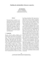
3.3. Bark factor model
No relationship was found between the estimated pa-
rameters and the tree measurements. The general adjust-
ment (figure 3 and table IV) remained accurate. Residual
variance decreases as x increases, in contrast to other
studies where residual error was higher at the foot of the
tree [7, 37]. This is probably due to the difficulty of
accurately measuring bark thickness on very small
discs. The data were therefore weighted by x in order to

ensure the equal distribution of studentised residuals
(figure 4). The values obtained for the parameters, with
their asymptotic standard error in parentheses, are the
following:
c
1
= 1.0532 (0.00366)
c
2
= 0.1580 (0.00457)
c
3
= 0.5656 (0.0231).
The model has an asymptote at c
1
> 1 which guaran-
tees that the model behaves logically (D
out
> D
in
). The
model fits the data observed rather well. The bark factor
tends towards infinity when the distance from the apex x
tends towards 0 but the model yields logical values very
quickly (D
out
/D
in
= 2 for x = 4 cm).
3.4. Evaluation of the modelled stem and ring

profiles on the independent dataset
3.4.1. Stem profiles
For 4 trees from the same stand in the Luberon region
(5329 measurements), we compared the annual stem
Profile and structure of Atlas cedar tree stem 71
Figure 2. Mean bias ((a), (b)) and mean error ((c), (d)) of stem profile models as a function of slenderness ratio (H/D).
profiles measured inside bark with the same profiles
modelled via two different approaches:
– integrated approach: we applied the outside bark stem
profile model and then the bark factor model to obtain
the annual inside bark profiles.
– incremental approach: we cumulatively applied the
ring area profile model onto the first basal area stem
profile which exceeded a height of 1.30 m.
For the 4 trees measured, the stem profile model IIa
with crown base gave the best overall results in terms
of bias and accuracy, followed by the ring profile
model and then the stem profile model IIb without
crown base (table V). These results should be modu-
lated according to the part of the tree being dealt with
(figure 5).At the butt level, the ring profile model gave
more accurate, and above all, less biased results than
the estimates made by the two stem profile models
72 F. Courbet and F. Houllier
Figure 3. Diameter outside bark/ diameter inside bark ratio (D
out
/D
in
) as a fonction of distance from tree top. Observations and fitted gen-
eral model.

Table IV. Accuracy of estimates using the bark factor model (1137 observations).
Model Weighted SSE Number of parameters DF Weighted RMSE
Individual model 1.08178 108 1031 0.032424
General model 3.33329 3 1134 0.054216
Table V. Mean bias and error observed when applying different models for predicting the stem profiles of 4 trees from a same stand
(5329 observations).
Model used Mean bias (mm) Mean error (mm)
Stem profile model with crown base (model IIa) 0.997 2.387
Stem profile model without crown base (model IIb) 1.835 2.976
Ring profile model applied to the estimation of the stem profile 1.783 2.588
which gave the same results at this level. Moving up-
wards along the stem, the behaviour of the ring profile
model worsens both in terms of bias and accuracy to
the point of performing worse atthe top of the tree than
the stem profile models. Similarly, the stem profile
model without crown base (IIb) becomes more biased
and less accurate than the stem profile model with
crown base (IIa) and gives mean estimates at this level
which are barely better than those of the ring profile
model.
Profile and structure of Atlas cedar tree stem 73
Figure 4. Studentized residuals of the general model of the bark factor (D
out
/D
in
) as a function of distance from tree top.
Figure 5. Application of the stem profile models (models IIa and IIb) and ring profile model to all the annual stem profiles of the 4 trees
in the Luberon region. Mean bias (a) and mean error (b) as a function of relative height class.
Figure 6 makes it possible to visually compare, for a
given tree, the results of the reconstruction of ring distri-

bution using the two methods.
3.4.2. Ring profiles
The measured annual ring width profiles were also
compared to the predicted ring profiles obtained by the
integrated and the incremental approaches.
The mean performances of the ring area profile model
are intermediate between those of the two stem profile
models in terms of bias but better in terms of accuracy
(table VI). The ring profile model is unbiased in the first
two thirds along the tree and, conversely, gives the most
biased estimates in the upper quarter of the tree. How-
ever, it is more accurate for the ring profile as a whole
(figure 7).
For instance, figure 8 shows two different rings from
the same tree, one of which is predicted more accurately
by the ring profile model, the other by the stem profile
model.
74 F. Courbet and F. Houllier
Figure 6. Observed distribution of ring widths for tree 1 in the Luberon region (a), reconstructed by superimposing the rings modelled by
the ring profile model (b) and by superimposing the stem profiles modelled by the stem profile model IIa (c).
Table VI. Mean bias and error observed when applying the different models for predicting ring width profiles for 4 trees from a same
stand (5329 observations).
Model used Mean bias (mm) Mean error (mm)
Stem profile model with crown base (model IIa) 0.070 0.386
Stem profile model without crown base (model IIb) 0.104 0.390
Ring profile model 0.081 0.305
Profile and structure of Atlas cedar tree stem 75
Figure 7. Application of the stem profile model (models IIa and IIb) and the ring profile model to the ring profiles of the 4 trees in the
Luberon region. Mean bias (a) and mean error (b) as a fonction of relative height class.
Figure 8. Observed 1982 and 1985 ring width profiles of tree 1 in the Luberon region, and those reconstructed by the difference between

successive annual stem profiles (models IIa and IIb) and by the ring profile model.
Table VII. Accuracy of the estimates obtained using the sapwood profile model (1095 observations).
Model SSE Number of parameters DF RMSE
Individual model 0.286395 2 × 30 1035 0.01663
General model 2.261983 2 1093 0.04549
3.5. Sapwood profile model
An initial individual model was constructed for each
tree. Relationships between the two parameters and cer-
tain tree characteristics (number of rings, width and area
of the sapwood at x
h
, tree variables) were then examined.
The parameter x
h
varied less between trees than the num-
ber of rings at the corresponding level (coefficient of
variation of 26.9% as opposed to 30.9%). Similarly, vari-
ations between trees of parameter b
1
could not be associ-
ated with any variable or combination of variables at tree
or stand level.
A general model simulating the evolution of the
sa
iba
ratio was therefore established for all the trees (figure 9),
even though it was less accurate than the individual
model (table VII). No bias was observed when we stud-
ied the distribution of the residuals according to disc
characteristics (mean number and width of the rings of

the disc, sapwood area, relative distance from the apex)
or tree characteristics (age, dimensions, crown base
height).
The values of the parameters, and their asymptotic
standard error (in parentheses), of the general model are
the following:
x
h
= 4.85 (0.078) m
e
1
= 0.0448 (6 x 10
–4
)m
–1
.
4. DISCUSSION
Two stem profile models were tested. They require ei-
ther the corrected slenderness ratio ((H – 1.30)/D ratio),
or the proportion of live crown. In the absence of artifi-
cial pruning of green branches, the two variables are
closely related because they both depend on the competi-
tion experienced by the tree during growth. The crown
base height model confirms that: the nearer the green
crown base is to the ground, the more conical the tree and
the greater the taper (Eq. (6)). Even so, knowing the
crown base height improves the accuracy of stem profile
predictions compared to only taking into consideration
the slenderness ratio, particularly near the top of the tree,
76 F. Courbet and F. Houllier

Figure 9. Relative sapwood area as a function of distance from the top. Observations and fitted general model. The value predicted by
the model is equal to 1 when the distance from the top is less or equal to 4.85 m.
which coincides with the results of other studies carried
out on Pinus taeda [5, 41].
The equation which uses the (H – 1.30)/D ratio none-
theless has greater scope because, not only can it be ap-
plied to trees for which the diameter and total height are
known, but also to artificially pruned trees, since in this
case the crown base is no longer that of the crown from
which the tree developed. The slenderness ratio, as well
as the stem profile, usually integrates tree growth before
and, if such is the case, after pruning.
Conversely, it is more logical for the ring profile
model to include crown base height since it is an incre-
ment model whose profile depends more on the position
of the photosynthetic apparatus than on the initial tree
form. It is thereby adapted to artificial pruning situations
which cause sudden variations in the extent and vertical
distribution of annual increment.
The selected stem profile model has only a few param-
eters. Considering the well-balanced sample, it is well
adapted to Atlas cedar. When applied to the 4 indepen-
dent validation trees, it shows that the bias and error of
the estimate are greater at the butt level and that the ad-
vantage of using the model with crown base height lies in
its greater ability to describe the upper part of the profile.
This rather simple model should be tested on other conif-
erous species. The number of parameters could be re-
duced even further if b
1

is no longer statistically different
from 1.
Although calculating the diameter at a given height
poses no problem, it is not possible to analytically com-
pute the height corresponding to a given diameter. Fur-
thermore, this model cannot be integrated analytically to
calculate the volume up to any given height or top diame-
ter limit. Nonetheless, approximate calculations by itera-
tion are possible and give perfectly satisfactory results.
It was possible to obtain the annual stem profiles of
4 trees by both the integrated and incremental ap-
proaches. Conversely, all the ring width profiles were
also predicted using these two approaches. (1) In both
cases, the reconstruction of the ring width distributions
gives compatible results: the profiles do not intersect and
do not generate negative increments. (2) Overall, the ring
profile model is more accurate than the stem profile
model for predicting ring profiles, whereas the stem pro-
file model is more accurate than the ring profile model
for predicting stem profiles. In other words, each profile
model proves to be more accurate when used directly to
predict the type of profile againstwhich it was calibrated.
(3) The accuracy of the models usually differs depending
on the part of the tree being dealt with: the ring profile
model gives better results for the butt and the lower part
of the stem both for the stem profiles and ring profiles
(but poorer results for the upper part of the tree): this
model behaviour is interesting in that it is for this part of
the trunk that the performance of the stem profile models
is the least successful [52], whereas this part is of greatest

interest in commercial terms.
The use of static stem profile equations for generating
increment values is in theory open to criticism. This
method goes hand in hand with the use of derivatives of
volume equations for calculating volume increment,
whereas they are not intended for this purpose. There is
no proof that these volume or profile equations are suit-
able for describing the evolution of the volume or shape
of trees over time. Just as a stand can refer to different
volume tables during development, one single profile
equation does not necessarily take into consideration the
evolution in stem form. For this reason, increment mod-
els are, in theory, preferable. This study also shows their
superiority when applied in practice.
The models were only tested on 4 trees from the same
stand. This test should berepeated on a greater number of
trees, particularly trees taken from different stands. In-
deed, trees taken from the same plot, regardless of their
social status, often have stem profiles or ring profiles
which exhibit the same tendencies (e.g. greater or lesser
butt) which means that they resemble each other to a
greater extent than trees from another stand. Trees are not
independent in the statistical sense of the word. Cunia
[12] showed that this could result in considerable dis-
crepancies between the biomass measured and the bio-
mass modelled at the stand level, which were in any case
much greater than those deduced from the theoretical
variances of the model. We therefore come across the
same problem here when studying tree form. Another
statistical problem, autocorrelation between errors, has

not been taken into consideration in this article.
Using the ring profile model improves the bias of the
estimates for the tree butt. No doubt because of its seg-
mented formulation, this model seems to be able to take
into consideration sudden changes in diameter at this
level more easily than stem profile models which gener-
ate smoother profiles. Nonetheless, the mean error of the
estimates for the butt remains considerable. This part of
the tree indeed varies greatly: on the one hand, the diame-
ter varies greatly within a short distance; on the other
hand, its form varies greatly between trees. Yet this part
of the trunk is the most valuable commercially and is
therefore the part which requires greater accuracy when
simulating wood quality. Therefore it would be necessary
Profile and structure of Atlas cedar tree stem 77
to sample more trees and also more discs within this part
of the tree in order to improve the accuracy of these mod-
els, particularly in order to find the segmentation point x
2
which determines the top of the butt in the ring profile
model.
For the sapwood area proportion profile, the simple
models (constant number of rings or sapwood width be-
low the point where the heartwood has formed) have
proved to be inefficient. Their advantage is limited to
only a small variety of situations in terms of age and
growth conditions [15]. Our sample of 30 stems was
noteworthy in that it represented a wide range of
silvicultural situations. But it is undoubtedly incomplete
and therefore unsuitable for being applied generally. Par-

ticularly, we were lacking in data for old trees over
100 years of age.
According to the pipe model theory, the sapwood
cross-sectional area, particularly if measured at the
crown base rather than at 1.30 m, is a good predictor of
leaf area and leaf biomass in trees of different sizes, with
more or less developed crowns [4, 33, 45]. Similarly,
within a tree, the sapwood cross-sectional area varies
from top to bottom of the crown in proportion to the leaf
area situated above it [22, 58, 59]. These relationships are
not always as simple or as strong as the pipe model pre-
dictions. A significant vigour effect is often observed, ei-
ther directly or via other factors such as climate [3], site
index [29], stand density [29, 57, 62] or silvicultural
practices [24, 28], either because the functional sapwood
often only represents part of the totalsapwood or because
the specific conductivity of the functional sapwood var-
ies depending on cambial age or social status [17, 54, 55].
The bark factor model was weighted by distance from
the apex. This weighting results in greater importance
being given to observations at the lower part of the tree,
which has the greatest economic value. It is also the part
which is most subjected to harmful effects in the case of a
fire, whether prescribed or not, and against which the
bark has a protective role [51].
The aim of obtaining a coherent set of allometric rela-
tionships which describe the internal structure of a trunk
has been reached. The models proposed can easily be
connected to the outputs of an individual tree growth
model which would predict the diameter and height of

each tree. The models are compatible and have been for-
mulated so as to make them behave logically: the stem
and ring profile models pass through the points located at
tree tip and at 1.30 m; the bark factor is always above 1;
the sapwood area ratio varies between 0 and 1 and is
equal to 1 above the level at which the heartwood
forms; the crown base height, varies between 0 and total
height H.
These characteristics which are essential in order to
determine the lumber yield and the behaviour of pro-
cessed wood, are not the only features which may be of
interest. These models only make it possible to simulate
the internal structure of defect free trees. With respect to
the stem, it is also useful to know the amount of defect,
the pith position (an eccentric pith is often associated
with the curve of the trunk) and the grain angle. These
features should be stochastically modeled, because we do
not know what determines them.
Branching is also largely responsible for the heteroge-
neity of the material because of the extent and shape of
the knots. A large number of studies have established the
determining influence of growth conditions on these
characteristics [9, 34, 38]. The internal trunk structure
should therefore also be completed by taking into consid-
eration other aspects, in particular branching.
The proposed models are probably valid for Lebanon
cedar (Cedrus libani A. Richard), which is very common
in Turkey and has a similar form. According to Quezel
[49], this species and the Atlas cedar are one and the
same. The form of the models proposed should be suit-

able also for a good number of other coniferous species
provided that reparameterisation is undertaken.
5. CONCLUSION
This study updates the situation regarding the model-
ling of the form and internal structure of trunks, by
proposing a series of allometric models which are com-
patible in terms of stem, ring, bark and sapwood profiles.
Some models (ring and sapwood profiles in particular)
should be validated or reparameterised on more substan-
tial samples so that they can be used more widely.
These data, together with the way they are synthesised
in model form, make it possible to increase our knowl-
edge on the way in which a tree develops and functions.
The relationships obtained are to be connected to out-
puts of a future tree growth model, so as to simulate the
form and internal structure of the stems. The different
profiles provided here can be predicted from simple and
standard tree measurements: total height, diameter at
1.30 m, and if needed the height of the live crown base.
78 F. Courbet and F. Houllier
Acknowledgements: This work was partially sup-
ported by a grant from the French Ministry of Agriculture
(DERF Convention 01.40.37/99). We are grateful to
Frédéric Jean, Nicolas Mariotte, Dominique Riotord and
Maurice Turrel for technical and field assistance and to
the national forest service (ONF) for providing the sam-
ple trees without payment. Wewish to thank Anne-Marie
Wall from the linguistic service of INRA for her great
help in the translation of this paper. We would also thank
two anonymous reviewers for their comments and sug-

gestions, and Stephen Hallgren for language review and
suggestions.
REFERENCES
[1] Bariteau M., Courbet F., Dreyfus Ph., Ducrey M., Du
Merle P., Fady B., Oswald H., Teissier du Cros E., Faut-il boiser
en région méditerranéenne ?, Forêt-entreprise 93 (1993) 24–45.
[2] Bergqvist G., Wood density traits in Norway spruce un-
derstorey: effects of growth rate and birch shelterwood density,
Ann. Sci. For. 55 (1998) 809–821.
[3] Berniger F., Nikinmaa E., Foliage area – sapwood area re-
lationships of Scots pine (Pinus sylvestris) trees in different cli-
mates, Can. J. For. Res. 24 (1994) 2263–2268.
[4] Blanche C.A., Hodges J.D., Nebeker T.E., A leaf area
– sapwood area ratio developed to rate loblolly pine tree vigor,
Can. J. For. Res. 15 (1985) 1181–1184.
[5] Burkhart H.E., Walton S.B., Incorporating crown ratio
into taper equations for loblolly pine trees, For. Sci. 31 (1985)
478–484.
[6] Cao Q.V., Burkhart H.E., Max T.A., Evaluation of two
methods for cubic-volume prediction of loblolly pine to any mer-
chantable limit, For. Sci. 26 (1980) 71–80.
[7] Cao Q.V., Pepper W.D., Predicting inside bark diameter
for shortleaf, loblolly, and longleaf pines, South. J. Appl. For.
10 (1986) 220–224.
[8] Clutter J.L., Compatible growth and yield models for lo-
blolly pine, For. Sci. 9 (1963) 354–371.
[9] Colin F., Houllier, F. Branchiness of Norway spruce in
northeastern France: predicting the main crown characteristics
from usual tree measurements, Ann. Sci. For. 49 (1992)
511–538.

[10] Courbet F., A three-segmented model for the vertical
distribution of annual ring area. Application to Cedrus atlantica
Manetti, For. Ecol. Manag. 119 (1999) 177–194.
[11] Coyea M.R , Margolis H.A., Gagnon R.R., A method
for reconstructing the development of the sapwood area of bal-
sam fir, Tree Physiol. 6 (1990) 283–291.
[12] Cunia T., On the error of tree biomass regressions: trees
selected by cluster sampling and double sampling, in: Estimating
tree biomass regressions and their error, Proc. Workshop on tree
biomass regression functions and their contribution to the error
of forest inventories estimates, May 26–30, 1986, Syracuse,
New York, 1986, pp. 49–59.
[13] Deleuze C., Houllier F., Prediction of stem profile of Pi-
cea abies using a process-based tree growth model, Tree Physiol.
15 (1995) 113–120.
[14] Demaerschalk J.P., Kosak A., The whole-bole system: a
conditionned dual-equation system for precise prediction of
tree profiles, Can. J. For. Res. 7 (1977) 488–497.
[15] Dhôte J F., Hatsch E., Rittié D., Profil de la tige et géo-
métrie de l’aubier chez le Chêne sessile (Quercus petraea Liebl),
Bull. Techn. ONF 33 (1997) 59–82.
[16] Dyer M.E., Burkhart H.E., Compatible crown ratio and
crown height models, Can. J. For. Res. 17 (1987) 572–574.
[17] Ewers F.W., Cruiziat P., Measuring water transport and
storage, in: Lassoie J.P., Hinckley T.M (Eds.), Techniques and
Approaches in Forest Tree Ecophysiology, CRC Press, Boca Ra-
ton, Louisiana, 1991, pp. 91–115.
[18] Fonweban J.N., Houllier F., Tarifs de cubage et fonc-
tions de défilement pour Eucalyptus saligna au Cameroun, Ann.
Sci. For. 54 (1997) 513–527.

[19] Forslund R.R., The power function as a simple stem pro-
file examination tool, Can. J. For. Res. 21 (1990) 193–198.
[20] Fowler G.W., Damschroder L.J., A red pine bark factor
equation for Michigan, North. J. Appl. For. 5(1) (1988) 28–30.
[21] Gjerdrum P., Prediction of heartwood in Pinus sylves-
tris, in: Nepveu G. (Ed), Proc. 3rd Workshop: Connection
between silviculture and wood quality through modelling ap-
proaches ans simulation software, September 5–12, 1999, La
Londe-Les-Maures, 1999, pp. 145–148.
[22] Gilmore D.W., Seymour R.S., Maguire D.A., Foliage
– sapwood area relationships for Abies balsamea in central
Maine, U.S.A, Can. J. For. Res. 26 (1996) 2071–2079.
[23] Gordon A., Estimating bark thickness of Pinus radiata,
N. Z. J. For. Sci. 13 (1983) 340–353.
[24] Granier A., Etude des relations entre la section du bois
d’aubier et la masse foliaire chez le Douglas (Pseudotsuga men-
ziesii Mirb. Franco), Ann. Sci. For. 38 (1971) 503–512.
[25] Guay, R., Gagnon, R., Morin, H., A new automatic and
interactive tree ring measurement system based on a line scan ca-
mera, For. Chron. 68 (1992) 138-141.
[26] Houllier F., Leban J M., Colin F., Linking growth mo-
delling to timber quality assessment for Norway spruce, For.
Ecol. Manage. 74 (1995) 91-102.
[27] Kozak A., A variable exponent taper equation, Can. J.
For. Res. 18 (1988) 1363–1368.
[28] Långström B., Hellqvist C., Effects of differents pruning
regimes on growth and sapwood area of Scots pine, For. Ecol.
Manag., 44 (1991) 239–254.
[29] Long J.N., Smith F.W., Leaf area – sapwood area rela-
tions of lodgepole pine as influenced by stand density and site in-

dex, Can. J. For. Res. 18 (1988) 247–250.
[30] Maguire D.A., Hann D.W., The relationship between
gross crown dimensions and sapwood area at crown base in Dou-
glas-fir, Can. J. For. Res. 19 (1989) 557-565.
Profile and structure of Atlas cedar tree stem 79
[31] Maguire D.A., Hann D.W., Bark thickness and bark vo-
lume in Southern Oregon Douglas-Fir, West. J. Appl. For. 5
(1990) 5–8.
[32] Maguire D.A., Battista J.L.F., Sapwood taper models
and implied sapwood volume and foliage profiles for coastal
Douglas-fir, Can. J. For. Res. 26 (1996) 849–863.
[33] Mäkelä A., Virtanen K., Nikinmaa E., The effects of ring
width, stem position, and stand density on the relationship bet-
ween foliage biomass ans sapwood area in Scots pine (Pinus syl-
vestris), Can. J. For. Res. 25 (1995) 970–977.
[34] Mäkinen H., Effect of stand density on radial growth of
branches of Scots pine in southern and central Finland, Can. J.
For. Res. 29 (1999) 1216–1224.
[35] Marquardt, D.W., An algorithm for least squares estima-
tion of non linear parameters, J. Soc. Indust. App. Math. 11
(1963) 431–441.
[36] Max T.A., Burkhart H.E., Segmented Polynomial Regres-
sion Applied to Taper Equations, For. Sci. 22 (1976) 283–289.
[37] Meredieu C., Croissance et branchaison du Pin laricio
(Pinus nigra Arnold ssp. Laricio (Poiret) Maire). Elaboration et
évaluation d’un système de modèles pour la prévision de caracté-
ristiques des arbres et du bois. Thèse de Doctorat, Université
Claude Bernard Lyon I, 1998.
[38] Meredieu C., Colin F., Herve J. C. Modelling branchiness
of Corsican pine with mixed-effect models (Pinus nigra Arnold

ssp. laricio (Poiret) Maire), Ann. Sci. For. 55 (1998) 359–374.
[39] Meredieu C., Colin F., Dreyfus Ph., Leban J M. A chain
of models from tree growth to properties of boards for Pinus ni-
gra ssp. laricio Arn.: simulation using CAPSIS (c) INRA and
WinEpifn (c) INRA. in: Nepveu G. (Ed.), Proceedings of the
third workshop: Connection between silviculture and wood qua-
lity through modelling approaches ans simulation software, Sep-
tember 5-12, 1999, La Londe-Les-Maures, 1999, pp. 505–513.
[40] Meyer H.A., Bark volume determination in trees, J. For.
44 (1946) 1067–1070.
[41] Muhairwe C.K., LeMay V.M., Kozak A., Effects of ad-
ding tree, stand, and site variables to Kozak’s variable-exponent
taper equation, Can. J. For. Res. 24 (1994) 252–259.
[42] Nepveu G., Blachon J L., Largeur de cerne et aptitude à
l’usage en structure de quelques conifères: Douglas, Pin syl-
vestre, Pin maritime, Epicea de Sitka, Epicéa commun, Sapin
pectiné. Rev. For. Fr. XLI 6 (1989) 497–506.
[43] Newberry J.D., Burkhart H.E., Variable-form stem pro-
file models for loblolly pine, Can. J. For. Res. 16 (1986)
109–114.
[44] Newnham R.M., Variable-form taper functions for four
Alberta tree species, Can. J. For. Res. 22 (1992) 210–223.
[45] O’Hara K.L., Valappil N.I., Sapwood – leaf area prediction
equations for multi-aged ponderosa pine stands in western Montana
and central Oregon, Can. J. For. Res. 25 (1995) 1553–1557.
[46] Ojansuu R., Maltamo M., Sapwood and heartwood taper
in Scots pine stems, Can. J. For. Res. 25 (1995) 1928–1943.
[47] Ormerod D.W., A simple bole model, For. Chron. 49
(1973) 136–138.
[48] Polge H., Influence de la compétition et de la disponibili-

té en eau sur l’importance de l’aubier du Douglas, Ann. Sci. For.
39 (1982) 379–398.
[49] Quezel P., Cèdres et cédraies du pourtour méditerranéen:
signification bioclimatique et phytogéographique, Forêt médi-
terranéenne XIX 3 (1998) 243–260.
[50] Ryan M.G., Sapwood volume for three subalpine coni-
fers: predictive equations and ecological implications, Can. J.
For. Res. 19 (1989) 1397–1401.
[51] Ryan K.C., Rigolot E., Botelho H., Comparative analy-
sis of fire resistance and survival of mediterranean and western
north american conifers, in: Proceedings of the 12th Conference
on Fire and Forest Meteorology, October 26–28, 1993, Jekyll
Island, GA,1994, pp. 701–708.
[52] Saint-André L., Leban J.M., Houllier F., Daquitaine R.,
Comparaison de deux modèles de profils de tige et validation sur
un échantillon indépendant. Application à l’Epicéa commun
dans le nord-est de la France. Ann. For. Sci. 56 (1999) 121–132.
[53] SAS Institute Inc., SAS/STAT user’s guide, version 6,
fourth edition. SAS Institute Inc., Cary, NC, USA, 1990.
[54] Shelburne V.B., Hedden R.L., Effect of stem height, do-
minance class, and site quality on sapwood permeability in lo-
blolly pine (Pinus taeda L.), For. Ecol. Manag. 83 (1996)
163–169.
[55] Shelburne V.B., Hedden R.L., Allen R.M., The effect of
site, stand density, ans sapwood permeability on the relationship
between leaf area and sapwood area in loblolly pine (Pinus taeda
L.), For. Ecol. Manag. 58 (1993) 193–209.
[56] Thomas C.E., Parresol B.R., Simple, flexible, trigono-
metric taper equations., Can. J. For. Res. 21 (1991) 1132–1137.
[57] Thompson D.C., The effect of stand structure and stand

density on the leaf area – sapwood area relationship of lodgepole
pine, Can. J. For. Res. 19 (1989) 392–396.
[58] Waring R.H., Schoeder P.E., Oren R., Application of the
pipe model theory to predict canopy leaf area., Can. J. For. Res.
12 (1982) 556–560.
[59] Whitehead D., Edwards W.R.N., Jarvis P.G., Conduc-
ting sapwood area, foliage area, and permeability in mature trees
of Picea sitchensis and Pinus contorta, Can. J. For. Res. 14
(1984) 940–947.
[60] Wiant H.V., Wingerd D.E., Variation of DIB/DOB ra-
tios with height on hardwood trees, West Virginia For. Notes 11
(1984) 19–20.
[61] Yang K.C., Hazenberg G., Sapwood and heartwood
width relationship to tree age in Pinus banksiana, Can. J. For.
Res. 21 (1991) 521–525.
[62] Yang K.C., Hazenberg G., Impact of spacings on sap-
wood and heartwood thickness in Picea mariana (Mill.) B.S.P.
and Picea glauca (Moench.) Voss, Wood Fiber Sci. 24 (1992)
330–336.
[63] Yang K.C., Hazenberg G., Bradfield G.E., Maze J.R.,
Vertical variation of sapwood thickness in Pinus banksiana
Lamb. and Larix laricina (Du Roi) K. Koch, Can. J. For. Res. 15
(1985) 822–828.
80 F. Courbet and F. Houllier