Báo cáo toán học: " A note on the speed of hereditary graph properties" ppsx

A note on the speed of hereditary graph properties
Vadim V. Lozin
∗
DIMAP and Mathematics Institute
University of Warwick, Coventry CV4 7AL, UK

Colin Mayhill
Mathematics Institute
University of Warwick, Coventry CV4 7AL, UK

Victor Zamar aev
†
University of Nizhny Novgorod, Russia

Submitted: Jan 27, 2011; Accepted: Jul 27, 2011; Published: Aug 5, 2011
Mathematics Subject Classification: 05C30
Abstract
For a graph property X, let X
n
be the number of graphs with vertex set
{1, . . . , n} having property X, also known as the speed of X. A property X is
called factorial if X is hereditary (i.e. closed under taking induced subgraphs) and
n
c
1
n
≤ X
n
≤ n
c
2

n
for some positive constants c
1
and c
2
. Hereditary properties with
the speed slower than factorial are surprisingly well structured. The situation with
factorial properties is more complicated and less exp lored, although this family in-
cludes many properties of theoretical or practical importance, such as planar graphs
or graphs of b ou nded vertex degree. To simplify the study of factorial properties, we
propose the following conjecture: the speed of a hereditary property X is factorial if
and only if the fastest of the following three properties is factorial: bipartite graphs
in X, co-bipartite graphs in X and split graphs in X. In this note, we verify the
conjecture for hereditary properties defined by forbidden induced subgraphs with
at most 4 vertices.
Keywords: Hereditary class of graphs; Speed of hereditary properties; Factoria l class
∗
Research of this author was supported by the Centre for Discrete Mathematics and Its Applications
(DIMAP), University of Warwick.
†
Research of this author was supported by RFFI, project number 11-01-001 07-a and by FAP “Research
and educational specialists of innovative Russia”, project number 2010-1.3.1-111-017-012
the electronic journal of combinatorics 18 (2011), #P157 1
1 Introduction
A graph property is an infinite class of graphs closed under isomorphism. A property is
hereditary if it is closed under taking induced subgraphs. Given a hereditary property X,
we write X
n
for the number of graphs in X with vertex set {1, 2, . . . , n}. Following [5], we
call X

n
the speed of the property X. In [1], it was proved that for any infinite hereditary
class X different from the class of all graphs,
lim
n→∞
log
2
X
n

n
2

= 1 −
1
k(X)
, (1)
where k(X) is a natural number called the index of the class X. To define this notion,
let us denote by E
i,j
the class of gra phs whose vertices can be partitioned into at most i
independent sets and j cliques. In particular,
• E
2,0
is t he class of bipartite graphs,
• E
1,1
is t he class of split graphs,
• E
0,2

is t he class of graphs complement to bipartite.
Then the index k(X) of a class X is the maximum k such that X contains a class E
i,j
with i + j = k. Now let us extend this definition by assuming that the index of every
finite hereditary class is 0, and the index o f t he class of all gra phs equals infinity. With
this extension, the family of all hereditary classes is partitioned into countable number
of subsets each of which consists of classes with the same index. Moreover, the classes
E
i,j
with the same value of i + j are the only minimal classes in the respective subset. In
particular, for k = 2, there are exactly three minimal classes: bipartite, complements of
bipartite, and split g raphs. Therefore, a n infinite hereditary class of graphs has index 1
if and only if it contains none of the three listed classes. The classes of index 1 have been
called in [2] unitary.
The family of unitary classes is of sp ecial interest, since it conta ins many classes
of theoretical and practical importance, such as interval graphs, permutation gr aphs,
chordal bipartite graphs, line graphs, forests, threshold graphs, all classes of graphs of
bounded vertex degree, o f bounded clique-width [4], all proper minor-closed graphs classes
(including planar graphs) [12], etc. In order to provide a differentiation of the unitary
classes in accordance with their size, let us introduce the following definition: two graph
classes X and Y will be called isometric if there are positive constants c
1
, c
2
and n
0
such
that Y
c
1

n
≤ X
n
≤ Y
c
2
n
for any n > n
0
. Clearly the isometricity is an equivalence relation.
The equivalence classes of this relation are called layers.
All finite classes of graphs constitute a single layer, and all classes of index greater
than 1 also constitute a single layer. Between these two extremes lies the family of unitary
classes, and it consists of infinitely many layers. The first four lower layers in this family
have been distinguished in [13]:
• constant layer contains classes X with log
2
|X
n
| = O(1),
the electronic journal of combinatorics 18 (2011), #P157 2
• polynomial layer contains classes X with log
2
|X
n
| = Θ(log
2
n),
• exponential layer contains classes X with log
2

|X
n
| = Θ(n),
• factorial layer contains classes X with log
2
|X
n
| = Θ(n log
2
n).
Independently, the same result was obtained by Alekseev in [2]. Moreover, Alekseev
provided the first fo ur layers with the description of all minimal classes and proposed
a structural characterization of the classes in the first three layers (some more involved
results can be found in [5, 6]). This characterization shows that the classes in t he three
lower layers have a rather simple structure. In pa rt icular, for any exponential class X
there is a constant c such that the vertices of any graph in X can be partitioned into at
most c subsets so that each of the subsets is either a clique or an independent set, and
between any two of them there are either all possible edges or none of them.
The factorial layer is substantially richer. It contains most of the unitary classes
mentioned above (t he unique exception in the above list is the class of chordal bipartite
graphs, which is superfactorial [14]). However, no complete structural characterization is
available for this layer. As a step towa r d this characterization, we propose the following
conjecture.
Conjecture A hereditary grap h property X i s factorial if and only if the fastest of the
following three properties is factorial: X ∩ E
2,0
, X ∩ E
1,1
, X ∩ E
0,2

.
This conjecture is suggested by the exceptional role o f the three minimal non-unitary
classes in the study of lower layers of hereditary properties. In particular, all minimal
classes in the first four layers are subclasses of bipartite, co-bipartite or split graphs.
Therefore, if we replace in the conjecture the factorial layer by any of the first t hree
lower layers, it becomes a valid statement. For the factorial layer, only one part of the
conjecture is known to be true ( the “only if” part), since all minimal factorial classes are
sub classes of bipartite, co-bipartite or split graphs. The three minimal factorial classes of
bipartite graphs ar e [2]:
• P
1
= F ree(K
3
, K
1,2
) (the notations are given below), the class of graphs of vertex
degree at most 1,
• P
2
, the class of “bipartite complements” of graphs in P
1
, i.e. the class of bipartite
graphs in which every vertex has at most one non-neighbor in the opposite part,
• P
3
= F ree(C
3
, C
5
, 2K

2
), the class of 2K
2
-free bipartite graphs, also known as chain
graphs for the property that the neighborhoods of vertices in each part form a chain.
The complements of graphs in P
1
, P
2
, P
3
form the three minimal factorial classes of
co-bipartite graphs. The remaining three minimal factorial classes also are closely related
to P
1
, P
2
, P
3
. To reveal this relationship, let us observe that by creating a clique in one
of the parts of a bipartite graph we obta in a split graph. By applying this operation to
graphs in P
1
, P
2
, P
3
, we transform t hese classes into sub classes of split graphs, which
are precisely the three remaining minimal factorial classes. For instance, the class P
3

the electronic journal of combinatorics 18 (2011), #P157 3
transforms in this way into the subclass of split graphs known as thresh old graphs, or
equivalently, ( 2K
2
, C
4
, P
4
)-free graphs.
To verify the “if” part of the conjecture, we initiate a systematic study a factorial
properties based on their induced subgraph characterization. It is well-known ( and not
difficult to see) that a graph property X is hereditary if and only if it can be described by
a set of forbidden induced subgraphs. In this paper, we show that the above conjecture
is true for all properties defined by forbidden induced subgraphs with at most 4 vertices,
which is the main result of the paper. The o r ganization of the paper is as follows. In the
rest of this section we introduce basic notations. In Section 2, we verify the conjecture
for all factorial classes defined by forbidden induced subgraphs on at most 4 vertices with
one exception. The only exception is the class of (K
1,3
, C
4
)-free graphs. We study this
class in Section 3, where we prove that this class is factorial.
We use the following notations. For a set of graphs M we denote by F ree(M) the
class o f graphs containing no induced subgraphs isomorphic to graphs in the set M and
call the g raphs in this class M -free.
For a graph G, we denote by V (G) and E(G) the vertex set and the edge set of G
respectively. The neighborhood N(v) of a vertex v ∈ V (G) is the set of vertices adjacent
to v. If N(v) is a clique, then v is a simplicial vertex. The subgraph of G induced by a
set U ⊆ V (G) is denoted G[U], and G \ U stands for G[V (G) \ U]. As usual, C

n
, P
n
and
K
n
denote the cycle, the path and the complete graph on n vertices respectively. Also, by
K
n,m
we denote a complete bipartite graph with parts of size n and m. An n-wheel W
n
is
a g raph with n + 1 vertices obtained from a cycle C
n
by adding a dominating vertex, i.e.
a vertex adjacent to every vertex of the cycle. The complements of a graph G is denoted
G and is called co-G.
2 Classes of graphs defined by 4-vertex forbidden in-
duced subgraphs
To avoid triviality, we do not forbid gra phs on two vertices. Graphs with at least three
vertices will be called non-trivial.
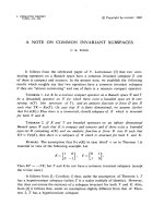
There are f our graphs on three vertices (triangle K
3
, path P
3
and their complements)
and eleven graphs on four vertices (listed in Figure 1).
In our analysis of classes defined by forbidden induced subgraphs we will use the
following two results.
Theorem 1. [4] Every class of graphs of bounded clique-width i s (at most) factorial.

Theorem 2. (see e.g. [3]) The class of C
4
-free bipartite graphs is superfactorial.
In particular, from Theorem 2 we derive the following necessary condition for a class
F ree(M) to be factorial (note t hat the class F ree(C
3
, C
4
) contains a ll C
4
-free bipartite
graphs).
the electronic journal of combinatorics 18 (2011), #P157 4
r r
rr
K
4
r r
rr
co-diamond
r r
rr
2K
2
= C
4
r r
rr
co-paw
r r

rr
❅
❅
❅
❅
co-claw
r r
rr
❅
❅
❅
❅ 



K
4
r r
rr
❅
❅
❅
❅
diamond
r r
rr
C
4
r r
rr

❅
❅
❅
❅
paw
r r
rr




claw
r r r r
P
4
Figure 1: All graphs on four vertices
Theorem 3. Let M be a set of graphs such that
• either M ∩ E
0,2
= ∅
• or M ∩ E
2,0
= ∅
• or M ∩ E
1,1
= ∅
• or M ∩ Free(C
3
, C
4

) = ∅
• or M ∩ Free(C
3
, C
4
) = ∅,
then F ree(M) is superfactorial.
Let us call the five classes listed in the theorem critical. In what follows, we show that
if M contains a graph in each of the critical classes and each graph in M has at most four
vertices, then F ree(M) is ( at most) factorial.
There is just one maximal graph contained in all five critical classes, namely a P
4
. It
is known (see e.g. [7]) that the clique-width of P
4
-free graphs is at most 2. Together with
Theorem 1 this gives a f actorial upper bound for the class F ree(P
4
). The class F ree(P
3
)
contains P
1
(one of the minimal factorial classes), which gives a lower bound. Therefore,
Theorem 4. The class F ree(G) is factorial i f and only if G is a non-trivial induced
subgraph of P
4
.
From now on, we assume that none of the forbidden graphs is an induced subgraph of
P

4
. This leaves us with 12 non-trivial graphs with at most four vertices none of which is
the electronic journal of combinatorics 18 (2011), #P157 5
an induced subgraph of P
4
. It is not difficult to see that each of them belongs to exactly
three of the five critical classes. We divide the set of these 12 graphs into four types
according to the critical classes they belong to:
(1) K
3
, K
4
, co-diamond, co-paw, claw belong to E
2,0
, E
1,1
, F ree(C
3
, C
4
).
(2) K
3
, K
4
, diamond, paw, co-cl aw belong to E
0,2
, E
1,1
, F ree(C

3
, C
4
).
(3) 2K
2
belongs to E
2,0
, E
0,2
, F ree(C
3
, C
4
).
(4) C
4
belongs to E
2,0
, E
0,2
, F ree(C
3
, C
4
).
Thus, a necessary condition fo r the class F ree(M) to be (at most) factorial is that the
set M contains at least two graphs: a graph of type (1) and a graph of type (2) or (4) (or
their complements). In what follows we show that this condition is also sufficient. Up to
symmetry and complementary arguments, we have 20 classes to analyze. Three of them

can be easily ruled out by the following observation:
• for any m and n, the class F ree(K
m
, K
n
) contains finitely many graphs due to
Ramsey Theorem.
It is not difficult to verify that the remaining 17 classes are at least factorial, since each
of t hem contains one of the minimal factorial classes. Now we turn to upper bounds.
First, we refer to some known results. In particular, in [7 ] it was proved that the
following gra ph classes and their complements have bounded clique-width and hence are
at most factorial:
• F ree(K
4
, co-paw ) ⊃ F ree(K
3
, co-paw ),
• F ree(K
4
, co-diamond) ⊃ F ree(K
3
, co-diamond),
• F ree(diamond, 2K
2
) ⊃ F ree(K
3
, 2K
2
),
• F ree(paw, claw) ⊃ F ree(K

3
, claw),
• F ree(diamond, co-diamond),
• F ree(diamond, co-paw),
• F ree(paw, 2 K
2
),
• F ree(paw, co-paw),
• F ree(co-claw, claw),
This reduces the analysis to the following 4 classes:
• F ree(K
4
, claw),
the electronic journal of combinatorics 18 (2011), #P157 6
• F ree(K
4
, 2K
2
),
• F ree(diamond, claw),
• F ree(co-claw, 2K
2
).
Theorem 5. The classes F ree(K
4
, claw), F ree(K
4
, 2K
2
), F ree(diamond, claw) are fac-

torial.
Proof. The lower bound follows fro m the fact that each of these classes contains at least
one minimal factorial class. For the upper bound we observe that
- the maximum vertex degree of graphs in F ree(K
4
, claw) is bounded by 5, since the
neighborhood of each vertex v is K
3
-free (else v belongs to a K
4
) and K
3
-free (else
v is the center of a claw). Therefore, there are at most n
5n
graphs with vertex set
{1, . . . , n} in the class F ree(K
4
, claw).
- the chromatic number of a 2K
2
-free graph G is bounded by

ω(G)+1
2

[15], where
ω(G) is the size of a maximum clique in G. Therefore, the vertices of a (K
4
, 2K

2
)-
free graph G can be partitioned into at most six independent sets. Each pair of the
independent sets induces a 2K
2
-free bipartite graph. Therefore, the edges of G can
be partitioned into at most 15 graphs each of which belongs to a f actorial class (i.e.
P
3
), which gives a factorial upper bound on the number of n-vertex labeled graphs
in F ree(K
4
, 2K
2
).
- Free(diamond, claw) is a subclass of the class of line graphs, which is factorial (see
e.g. [8]). Independently, a factorial upper bound on the number of graphs in the
class F ree(diamond, claw) can be obtained by observing that each vertex of a graph
in this class belongs to at most two maximal cliques, which shows that the number
of n vertex graphs in this class is at most n
2n
.
The class F ree(co-claw, 2K
2
) also is factorial, but the proof is more complicated and
we postpone it till the next section. Summarizing the above discussion, we obtain the
following conclusion.
Theorem 6. Let M be a set of graphs with at most four vertices such that F ree(M) is at
least factorial (i.e. contains one of the minimal factorial clas ses). Then F ree(M) is fac-
torial if and only if it contains non e of the five critical classes E

0,2
, E
2,0
, E
1,1
, F ree(C
3
, C
4
),
F ree(C
3
, C
4
).
the electronic journal of combinatorics 18 (2011), #P157 7
3 (Claw, Square)-free graphs
In the previous section we analyzed classes defined by forbidden induced subgraphs with
at most fo ur vertices and revealed all factorial classes in this family with one exception,
the class F ree(co-claw, 2K
2
). In this section, we study complements of graphs in F ree(co-
claw, 2K
2
), i.e. graphs which are claw-free and C
4
-free. It is not difficult to see that the
intersection of this class with each of the three minimal non-unitary classes is factorial.
Therefore, according to the conjecture in the intro duction, this class is factorial too. Below
we prove this fact. The proof is based on some structural characterizations of claw-free

graphs that can be found in the literature. In particular, the following theorem was proved
in [11].
Theorem 7. A graph is claw-free and 4-wheel -free if and only if the neighborhood of each
vertex is either the complement of a chain graph or a graph obtained from C
5
or W
5
by
duplication of some of i ts vertices (i.e. by substituting the vertices with cliques).
Obviously, F ree(K
1,3
, C
4
) is a subclass of F ree(K
1,3
, W
4
). Therefore, by Theorem 7,
the neighborhood of each vertex of a (K
1,3
, C
4
)-free graph induces either the complement
of a chain graph or a graph obtained from C
5
or W
5
by duplication of some of its vertices.
First o f all, let us show that without loss of generality we can reduce our analysis to
the case when the neighborhood of each vertex of a (K

1,3
, C
4
)-free graph induces the
complement of a chain gra ph.
Let G be a (K
1,3
, C
4
)-free graph and assume it contains a vertex x whose neighborhood
induces a graph obtained from a C
5
by duplicating some of its vertices. D enote A = N(x)
and B = V (G) \ (A ∪ {x}). We denote the cliques substituting the vertices of the C
5
by A
i
, i = 0, . . . , 4 with two cliques being adjacent if and only if their indexes differ by
exactly 1 (all additions are t aken mod 5). We will show that in order to describe the
graph we need to know G \ {x} and only one neighbor of x in each of the cliques. To this
end, let us prove the following lemma.
Lemma 1. Let a
i
∈ A
i
for i = 0, . . . , 4, then N(a
i−1
) ∩ N(a
i+1
) = A

i
∪ {x}.
Proof. Without loss of generality, let i = 2. It is clear that N(a
1
) ∩ N (a
3
) ∩ A = A
2
. Now
we show that N(a
1
) ∩ N(a
3
) ∩ B = ∅. Suppose not: then x, a
1
, a
3
and any vertex from
N(a
1
) ∩ N(a
3
) ∩ B would induce a C
4
, which is forbidden. This contradiction shows that
a
1
and a
3
have no common neighbors in B and therefore N(a

1
) ∩ N (a
3
) = A
2
∪ {x}.
From Lemma 1 it follows t hat N(x) = (

4
i=0
N(a
i−1
) ∩ N(a
i+1
)) \ {x}. Therefore, G
can be described by G \ {x} and five neighbors of x.
Assume now that a (K
1,3
, C
4
)-free graph G contains a vertex x whose neighborhood
induces a graph obtained from a W
5
by duplicating some of its vertices. Again we denote
A = N(x) and B = V (G) \ (A ∪ {x}). Also, let C be the clique substituting the central
vertex of the wheel and A
i
, i = 0, . . . , 4 the cliques substituting the remaining vertices o f
the wheel.
the electronic journal of combinatorics 18 (2011), #P157 8

Lemma 2. Let c ∈ C, then N(c) ∪ {c } = A ∪ {x}.
Proof. It is clear that N(c) ∪ {c} ⊇ A ∪ {x}. In order to prove the lemma we need to
show the reverse inclusion. Suppose to the contrary that there is a vertex y in B which is
adjacent to c. The neighbors of y in A induce a complete graph, since otherwise G would
contain an induced C
4
. Therefore, N(y)∩A ⊆ C ∪A
i
∪A
i+1
for some index i ∈ {0, . . . , 4}.
Without loss of generality let N(y) ∩ A ⊆ C ∪ A
1
∪ A
2
, but then c, y together with any
two vertices a
0
∈ A
0
and a
3
∈ A
3
would induce a K
1,3
. This contradiction proves the
lemma.
According to Lemma 2 in the graph G \ {x} the set N(c) ∪ {c} describes the neigh-
borhood of vertex x in the graph G. Therefore, to describe G we need to know G \ {x}

and an arbitrary vertex c ∈ C.
Now let us denote by Y the class of (K
1,3
, C
4
)-free graphs in which the neighborhood of
every vertex induces the complement of a chain graph. Obviously, this class is hereditary.
Lemma 3. Th e class F ree(K
1,3
, C
4
) is factorial if and only if Y is factorial.
Proof. If F ree(K
1,3
, C
4
) is factorial, then Y is factorial, because it is a proper subclass of
F ree(K
1,3
, C
4
) and it contains one of the minimal factorial classes ( the class of comple-
ments of chain graphs).
Conversely, suppose that Y is a factorial class and let G be an arbitrary n-vertex
graph in F ree(K
1,3
, C
4
). If G contains a vertex x
1

whose neighborhood induces either
a C
5
or a wheel W
5
, then we remove it from G and record x
1
and (at most) five of its
neighbors a
1
0
, a
1
1
, a
1
2
, a
1
3
, a
1
4
which allow us to describe the neighborhood of x
1
. After this
operation, we have a record containing at most 6 vertices and a graph G
1
obtained from
G by deleting x

1
. If G
1
contains a vertex x
2
whose neighborhood induces either a C
5
or
a wheel W
5
, we repeat the procedure which leaves us with a record conta ining at most
12 vertices and a graph G
2
obtained from G
1
by deleting x
2
. We repeat this procedure
until we obtain a gra ph G
k
from Y, where k ≤ n is the number of applications of the
operation. The record
x
1
, a
1
0
, a
1
1

, a
1
2
, a
1
3
, a
1
4
, . . . , x
k
, a
k
0
, a
k
1
, a
k
2
, a
k
3
, a
k
4
, G
k
, (2)
completely describes the graph G (i.e. allows to restore G from the record). Therefore,

the number of different records of typ e (2) equals the number of n-vertex labeled graphs
in F ree(K
1,3
, C
4
). Since G
k
is an (n − k)-vertex graph from a factorial class, an upper
bound on this number can be estimated as follows:
n

k=0
(n

n
5

5!)
k
(n − k)
c(n−k)
<
n

k=0
120
k
n
6k+c(n−k)
≤

n

k=0
120
k
n
max{6,c}n
< n
c
1
n
, (3)
where c
1
is constant. From (3) we conclude that F ree(K
1,3
, C
4
) is a factorial class.
Lemma 3 allows us to focus in the rest of the section on graphs in t he class Y, which
is precisely the class of C
4
-free quasi-line graphs.
the electronic journal of combinatorics 18 (2011), #P157 9
3.1 Quasi-line graphs without a square
A graph is a quasi - l i ne graph if the neighborhood of every vertex induces a co-bipartite
graph. Obviously, the class of quasi-line graphs is superfactorial, since it contains all
co-bipartite graphs. In this section, we study quasi-line graphs containing no C
4
as an

induced subgraph and show that this class is factoria l. A crucial role in our proof is
played by the structural characterization of quasi-line graphs proposed by Chudnovsky
and Seymour [9]. To describe this characterization we need to introduce a few definitions.
Circular interval graph.
Let C be a circle, V a finite set of points of C, and I a set of intervals of C (an interval
is a proper subset of C homeomorphic to [0, 1]). Define G to be the graph with vertex
set V and two vertices u, v ∈ V (G) being adjacent if and only if {u, v} is a subset of one
of the intervals. We call the triple (C, V, I) a circular interval representation of G. Any
graph that admits a circular interval representat io n is called a circ ular interva l graph. A
special case of circular interval graphs are linear interval graphs which are defined in the
same way with C being a line instead of a circle.
Fuzzy circular interval graph.
A graph G = (V, E) is a fuzzy circular interval if the following conditions hold:
1. There is a map φ from V (G) to a circle C (not necessarily injective).
2. There is a set of intervals I of C, none including another, such that no point of C
is an endpoint of more than one interval so tha t:
(a) If two vertices u and v are adjacent, then φ (u) and φ(v) belong to a common
interval.
(b) If two vertices u and v belong to a same interval, which is not an interval with
endpoints φ(u) and φ(v), then they are adjacent.
In other words, for a fuzzy circular interval graph the pair (φ, I) completely describe
adjacencies, except adjacencies for vertices u a nd v such that I contains an interval with
the endpoints φ(u) and φ(v). For such vertices adjacency is fuzzy. Note that if we require
φ to be injective, the definition of a fuzzy circular interval graph would be equivalent to
the definition of a circular interval graph. By replacing the circle C with a line we obtain
a definition o f a fuzzy linear in terva l graphs
Strip
A strip is a triple (G, a, b), where G is a graph and a, b are two designated simplicial
vertices of G called the ends of the strip. A strip (G, v
1

, v
n
), n > 1 is called a linear
interval strip if G is a linear interval graph with vertices v
1
, . . . , v
n
listed in the order of
their appearances in the linear interval representation of G. Fuzzy linear interval strips
are defined analogously, provided that if a, b are the endpoints of the strip then φ(a), φ(b)
are different from φ(v) f or all other vertices v of G.
the electronic journal of combinatorics 18 (2011), #P157 10
Composition of strips
The composition of two strips (G, a, b) and (G
′
, a
′
, b
′
) is the graph obtained from the union
of G \ {a, b} and G
′
\ {a
′
, b
′
} by adding to it all possible edges between N(a) and N(a
′
)
and between N(b) and N(b

′
).
Let G
0
be a disjoint union of complete graphs with an even number o f vertices whose
vertex set is partitioned into pairs of nonadjacent vertices, i.e. V (G
0
) = {a
1
, b
1
, . . . , a
k
, b
k
}
with a
i
being nonadjacent to b
i
for each i = 1, . . . , k. Also, for i = 1, . . . , k, let (G
′
i
, a
′
i
, b
′
i
)

be a collection of k strips that are vertex-disjoint, also from G
0
. For i = 1, . . . , k, let G
i
be the graph obtained by composing (G
i−1
, a
i
, b
i
) with (G
′
i
, a
′
i
, b
′
i
). The resulting graph
G
n
is called a composition of the strips (G
′
i
, a
′
i
, b
′

i
) (1 ≤ i ≤ k).
Chudnovsky and Seymour proved the following structural result in [9].
Theorem 8. A connected quasi-line graph G is either a fuzzy circular interval graph o r
a co mposition of fuzzy linear interval strips.
3.1.1 The structure of quasi-line graphs without C
4
In this section we show that the class of quasi-line graphs without a C
4
is obtained from
the class of quasi-line graphs by excluding the fuzziness from the definition.
Let G be fuzzy circular interval graph with a representatio n (φ, I). If [p, q] is an
interval of I such that φ
−1
(p) and φ
−1
(q) are b oth non-empty, then the pair of cliques
(φ
−1
(p), φ
−1
(q)) is called a fuzzy pair, where φ
−1
(p) denotes the clique {v ∈ V (G) | φ(v) =
p}. The following Lemma was proved in [10].
Lemma 4. Let G be a fuzzy circular interval graph with a repres entation (φ, I). If no
fuzzy pair contains an induced C
4
, then G is a circular interval graph.
As an immediate corollary from this lemma, we make the following conclusion.

Corollary 1. If G is a fuzzy circular interval graph containing no C
4
as an induced
subgraph, then G is a ci rcular interval graph.
Also, since a fuzzy linear interval graph is a special case of a fuzzy circular interval
graph, we conclude the following.
Corollary 2. If (G, a, b) is a fuzzy linear interval strip containing n o C
4
as an induced
subgraph, then (G, a, b) is a linear in terva l strip.
Now we show that if H is a composition of strips and H is a C
4
-free graph, then each
strip in the composition also is C
4
-free. Obviously, it suffices to prove this statement only
for two strips.
Lemma 5. Let H be the composition of two fuzzy linear interval strips (G
1
, a
1
, b
1
) and
(G
2
, a
2
, b
2

). If H is C
4
-free, then both strips are C
4
-free.
the electronic journal of combinatorics 18 (2011), #P157 11
Proof. Suppose without loss of g enerality that G
1
contains an induced C
4
. Since a
1
and b
1
are simplicial, they do not belong to any induced C
4
. Therefore, G
1
\{a
1
, b
1
} also contains
an induced C
4
. By definition, G
1
\ {a
1
, b

1
} is an induced subgraph of H. Therefore, H
also contains an induced C
4
, which contradicts the assumption.
Combining this lemma with Corollaries 1 and 2 and Theorem 8 we obtain the following
structural characterization of C
4
-free quasi-line graphs.
Theorem 9. A connected quasi-line graph G without an induced C
4
is either a circular
interval graph or a compo sition of linear interval strips.
3.1.2 The number of n-vertex quasi-line graphs without C
4
In this section we show that the class of C
4
-free quasi-line gr aphs is factorial. The lower
bound follows from the fact that this class contains P
1
(one of the minimal factorial
classes). Therefore, we only need to prove an upper bound. To this end, we may restrict
ourselves to connected graphs only.
We start by estimating the number of circular interval graphs. It is known (see e.g.
[9]) that this class is a proper subclass of the class of circular arc graphs. A graph G is a
circular arc graph if it is the intersection graph of a set I = {I
1
, . . . , I
n
} of intervals (arcs)

on a circle C, i.e. if there exists a one-to-one correspondence between the vertices of G
and the intervals of I such that two vertices of G are adjacent if and o nly if the respective
intervals intersect (without loss of generality, we may assume that no two intervals of I
share the same endpoint). The pair (C, I) is called a circular arc model of G. We call
two circular arc models different if they define different labeled graphs and equivalent
otherwise.
Lemma 6. Th e class of circular arc graphs is factorial .
Proof. The lower bound follows from the fact that this class contains P
1
. For the upper
bound, let G be an n-vertex circular arc graph and (C, I) a circular arc model representing
G with I = {[a
i
, b
i
], i = 1, . . . , n}. Starting from a
1
, we write out the labels of the
endpoints of intervals in the order t hey appear on the circle clockwise, which results in a
sequence
π
I
= [c
1
, c
2
, . . . , c
2n
], (4)
where every element of the sequence is either a

i
or b
i
for some value of i. In part icular,
c
1
= a
1
. It is clear that if π
I
= π
I
′
, then the models (C, I) and (C, I
′
) are equivalent,
i.e. they represent the same labeled graph. Therefore, the number of different circular
arc models does not exceed the number of different sequences of type (4), which is (2n)!.
Therefore, the class of circular arc graphs is factorial.
Corollary 3. The clas s of circular interval graphs and the class of l inear interval grap hs
are fa ctorial.
Proof. Corollary follows from the fact that both classes are subclasses of the class of
circular arc graphs and both of them contain P
1
(one of the minimal factorial classes).
the electronic journal of combinatorics 18 (2011), #P157 12
Now we turn to estimating the number of different labeled n-vertex compositions of
linear interval strips. Without loss of generality, we assume that every strip contains at
least 3 vertices, since otherwise it adds nothing to the composition and hence can be
ignored.

Any n-vertex composition of k strips is completely determined by
• a 2k-vertex labeled graph G
0
, which is a disjoint union of cliques, given together
with a partition of its vertices into pairs {a
1
, b
1
, . . . , a
k
, b
k
},
• an ordered list o f k labeled strips (G
′
i
, a
′
i
, b
′
i
) (i = 1 , . . . , k).
Note that k ≤ n, since each strip adds at least one vertex to the resulting graph. We
denote the number of vertices in the i-th strip by n
i
= t
i
+ 2, where t
i

is the number
of vertices the i-th strip contributes to the resulting graph. Therefore,

k
i=1
t
i
= n and
hence

k
i=1
n
i
= n + 2k ≤ 3n.
Let G = (V, E) be a n-vertex composition of k strips. The strips define an ordered
partition of V into k nonempty subsets. We fix this partition and estimate the number of
ways to compose G based on this partition. There are at most (2k)
2k
ways to create G
0
and at most (2k)
2k
ways to pair its vertices. If G is C
4
-free, then by Theorem 9 every strip
in the composition is linear interval. By Corollary 3, the class of linear interval graphs
is factorial and hence the number o f labeled linear interval strips on n
i
vertices does not

exceed n
cn
i
i
for a constant c. Therefore, for a fixed ordered partition of V into k nonempty
subsets, there are at most
(2k)
4k
k

i=1
n
cn
i
i
≤ (2n)
4n
n
P
k
i=1
cn
i
≤ n
11cn
ways to compose G = (V, E).
The number o f different o rdered par titio ns of V into k subsets does not exceed k
n
and therefore the total number of labeled n-vertex compositions of linear interval strips
is bounded by

n

k=1
n
11cn
k
n
≤ n
(11c+1)n+1
< n
c
1
n
,
for a constant c
1
. This fact together with Corollary 3 and Theorem 9 imply the following
conclusion.
Lemma 7. Th e class of C
4
-free quasi-line graphs is factorial.
Now from Lemmas 3 and 7 follows the main result of the section.
Theorem 10. The class F ree(K
1,3
, C
4
) is factorial.
the electronic journal of combinatorics 18 (2011), #P157 13
References
[1] V.E. Alekseev, Rang e of values of entropy of hereditary classes of graphs, Diskret.

Mat. 4 (199 2), no. 2, 148–157 (in Russian; translation in Discre te Mathematics and
Applications, 3 (1993), no. 2, 191 –199).
[2] V. Alekseev, On lower layers of the lattice of hereditary classes of graphs,
Diskretn. Anal. Issled. Oper. Ser. 1 Vol. 4 ,no. 1, (1997), 3-12 (in Russian).
[3] P. Alle n, Forbidden induced bipartite graphs, Journal of Graph Theory, 60 (2009)
219–241.
[4] P. Alle n, V. Lozin and M. Rao, Clique-width and the speed of hereditary prop-
erties, Electronic Journal of C ombinatorics, 16 (2009) Research Paper 35.
[5] J. Balogh, B. Bollob
´
as and D. Weinreich, The speed of hereditary properties
of graphs, J. Combin. Theory B, 7 9 (2000) 131-156.
[6] J. Balogh, B. Bollob
´
as and D. Weinreich, A jump to the Bell number for
hereditary graph properties, J. Combin. Theory S e r. B 95 (2005) 29–48.
[7] A. Brandst
¨
adt, J. Engelfriet, H O. Le and V.V. Lozin, Clique-Width for
4-Vertex Forbidden Subgraphs Theory of C omputing Systems, 34 (2006) 561–590.
[8] P. Cameron, T. Prellberg and D. Stark, Asymptotic enumeration of 2-covers
and line graphs, Discrete Mathematics, 310 (2010) 230–240.
[9] M. Chudnovsky and P. Seymour, The structure of claw-free graphs, London.
Math. Soc. Lecture Note Series, 327 (2005) 153-171.
[10] F. Eisenbrand, G. Oriolo, G. Stauffer and P. Ventura, The stable set
polytope of quasi-line graphs, Combinatorica, 28 (2008) 4 5–67.
[11] T. Kloks, K
1,3
-free and W
4

-free graphs, I nformation Processing Letters, 60 (199 6)
221–223.
[12] S. Norine, P. Seymour, R. Thomas and P. Wollan, Proper minor-closed
families are small, J. Combinatorial Theory B 96 (2006) 754–757 .
[13] E.R. Scheinerman and J. Zito, On the size of hereditary classes of graphs,
J. Combin. Theory B 61 (1994) 16–39.
[14] J.P. Spinrad, Nonredundant 1’s in Γ-free matrices, SIAM J. Discrete Math. 8
(1995) 25 1–257.
[15] S. Wagon, A bound on the chromatic number of graphs without certain induced
subgraphs, J. Combinatorial Theory B 29 (1980) 345–346.
the electronic journal of combinatorics 18 (2011), #P157 14