Electrical Power Systems Quality, Second Edition phần 2 ppsx

causing a voltage sag with duration of more than 1 cycle occurs within
the area of vulnerability. However, faults outside this area will not
cause the voltage to drop below 0.5 pu. The same discussion applies to
the area of vulnerability for ASD loads. The less sensitive the equip-
ment, the smaller the area of vulnerability will be (and the fewer times
sags will cause the equipment to misoperate).
3.2.3 Transmission system sag
performance evaluation
The voltage sag performance for a given customer facility will depend on
whether the customer is supplied from the transmission system or from
the distribution system. For a customer supplied from the transmission
system, the voltage sag performance will depend on only the transmission
system fault performance. On the other hand, for a customer supplied
from the distribution system, the voltage sag performance will depend on
the fault performance on both the transmission and distribution systems.
This section discusses procedures to estimate the transmission sys-
tem contribution to the overall voltage sag performance at a facility.
Section 3.2.4 focuses on the distribution system contribution to the
overall voltage sag performance.
Transmission line faults and the subsequent opening of the protec-
tive devices rarely cause an interruption for any customer because of
the interconnected nature of most modern-day transmission networks.
These faults do, however, cause voltage sags. Depending on the equip-
ment sensitivity, the unit may trip off, resulting in substantial mone-
tary losses. The ability to estimate the expected voltage sags at an
end-user location is therefore very important.
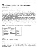
Most utilities have detailed short-circuit models of the intercon-
nected transmission system available for programs such as ASPEN*
One Liner (Fig. 3.7). These programs can calculate the voltage through-
out the system resulting from faults around the system. Many of them
can also apply faults at locations along the transmission lines to help

calculate the area of vulnerability at a specific location.
The area of vulnerability describes all the fault locations that can
cause equipment to misoperate. The type of fault must also be consid-
ered in this analysis. Single-line-to-ground faults will not result in the
same voltage sag at the customer equipment as a three-phase fault.
The characteristics at the end-use equipment also depend on how the
voltages are changed by transformer connections and how the equip-
ment is connected, i.e., phase-to-ground or phase-to-phase. Table 3.1
summarizes voltages at the customer transformer secondary for a sin-
gle-line-to-ground fault at the primary.
Voltage Sags and Interruptions 51
*Advanced Systems for Power Engineering, Inc.; www.aspeninc.com.
Voltage Sags and Interruptions
Downloaded from Digital Engineering Library @ McGraw-Hill (www.digitalengineeringlibrary.com)
Copyright © 2004 The McGraw-Hill Companies. All rights reserved.
Any use is subject to the Terms of Use as given at the website.
The relationships in Table 3.1 illustrate the fact that a single-line-
to-ground fault on the primary of a delta-wye grounded transformer
does not result in zero voltage on any of the phase-to-ground or
phase-to-phase voltages on the secondary of the transformer. The
magnitude of the lowest secondary voltage depends on how the
equipment is connected:
■
Equipment connected line-to-line would experience a minimum volt-
age of 33 percent.
■
Equipment connected line-to-neutral would experience a minimum
voltage of 58 percent.
This illustrates the importance of both transformer connections and
the equipment connections in determining the actual voltage that

equipment will experience during a fault on the supply system.
Math Bollen
16
developed the concept of voltage sag “types” to describe
the different voltage sag characteristics that can be experienced at the
end-user level for different fault conditions and system configurations.
The five types that can commonly be experienced are illustrated in Fig.
3.8. These fault types can be used to conveniently summarize the
52 Chapter Three
Figure 3.7 Example of modeling the transmission system in a short-circuit program for
calculation of the area of vulnerability.
Voltage Sags and Interruptions
Downloaded from Digital Engineering Library @ McGraw-Hill (www.digitalengineeringlibrary.com)
Copyright © 2004 The McGraw-Hill Companies. All rights reserved.
Any use is subject to the Terms of Use as given at the website.
Voltage Sags and Interruptions 53
0.58 1.00 0.58 0.00 1.00 1.00
0.58 1.00 0.58 0.33 0.88 0.88
0.33 0.88 0.88 — — —
0.88 0.88 0.33 0.58 1.00 0.58
TABLE 3.1 Transformer Secondary Voltages with a Single-Line-to-Ground
Fault on the Primary
Transformer
connection Phase-to-phase Phase-to-neutral Phasor
(primary/secondary) V
ab
V
bc
V
ca

V
an
V
bn
V
cn
diagram
Sag Type D
One-phase
sag, phase
shift
Sag Type B
One-phase
sag, no phase
shift
Phase
Shift
Angle
None
Sag Type C
Two-phase
sag, phase
shift
Sag Type E
Two-phase
sag, no phase
shift
Sag Type A
Three-phase
sag

Note: Three-phase sags
should lead to relatively
balanced conditions;
therefore, sag type A is a
sufficient characterization
for all three-phase sags.
Number of Phases
12 3
Figure 3.8 Voltage sag types at end-use equipment that result from different types of
faults and transformer connections.
Voltage Sags and Interruptions
Downloaded from Digital Engineering Library @ McGraw-Hill (www.digitalengineeringlibrary.com)
Copyright © 2004 The McGraw-Hill Companies. All rights reserved.
Any use is subject to the Terms of Use as given at the website.
expected performance at a customer location for different types of
faults on the supply system.
Table 3.2 is an example of an area of vulnerability listing giving all the
fault locations that can result in voltage sags below 80 percent at the cus-
tomer equipment (in this case a customer with equipment connected
line-to-line and supplied through one delta-wye transformer from the
transmission system Tennessee 132-kV bus). The actual expected per-
formance is then determined by combining the area of vulnerability with
the expected number of faults within this area of vulnerability.
The fault performance is usually described in terms of faults per 100
miles/year (mi/yr). Most utilities maintain statistics of fault perfor-
mance at all the different transmission voltages. These systemwide
statistics can be used along with the area of vulnerability to estimate
the actual expected voltage sag performance. Figure 3.9 gives an exam-
ple of this type of analysis. The figure shows the expected number of
voltage sags per year at the customer equipment due to transmission

system faults. The performance is broken down into the different sag
types because the equipment sensitivity may be different for sags that
affect all three phases versus sags that only affect one or two phases.
3.2.4 Utility distribution system sag
performance evaluation
Customers that are supplied at distribution voltage levels are impacted
by faults on both the transmission system and the distribution system.
The analysis at the distribution level must also include momentary
interruptions caused by the operation of protective devices to clear the
faults.
7
These interruptions will most likely trip out sensitive equip-
ment. The example presented in this section illustrates data require-
ments and computation procedures for evaluating the expected voltage
sag and momentary interruption performance. The overall voltage sag
performance at an end-user facility is the total of the expected voltage
sag performance from the transmission and distribution systems.
Figure 3.10 shows a typical distribution system with multiple feed-
ers and fused branches, and protective devices. The utility protection
scheme plays an important role in the voltage sag and momentary
interruption performance. The critical information needed to compute
voltage sag performance can be summarized as follows:
■
Number of feeders supplied from the substation.
■
Average feeder length.
■
Average feeder reactance.
■
Short-circuit equivalent reactance at the substation.

54 Chapter Three
Voltage Sags and Interruptions
Downloaded from Digital Engineering Library @ McGraw-Hill (www.digitalengineeringlibrary.com)
Copyright © 2004 The McGraw-Hill Companies. All rights reserved.
Any use is subject to the Terms of Use as given at the website.
Voltage Sags and Interruptions 55
TABLE 3.2 Calculating Expected Sag Performance at a Specific
Customer Site for a Given Voltage Level
Voltage at
Bus monitored
Fault type Faulted bus voltage bus (pu) Sag type
3LG Tennessee 132 0 A
3LG Nevada 132 0.23 A
3LG Texas 132 0.33 A
2LG Tennessee 132 0.38 C
2LG Nevada 132 0.41 C
3LG Claytor 132 0.42 A
1LG Tennessee 132 0.45 D
2LG Texas 132 0.48 C
3LG Glen Lyn 132 0.48 A
3LG Reusens 132 0.5 A
1LG Nevada 132 0.5 D
L-L Tennessee 132 0.5 C
2LG Claytor 132 0.52 C
L-L Nevada 132 0.52 C
L-L Texas 132 0.55 C
2LG Glen Lyn 132 0.57 C
L-L Claytor 132 0.59 C
3LG Arizona 132 0.59 A
2LG Reusens 132 0.59 C

1LG Texas 132 0.6 D
L-L Glen Lyn 132 0.63 C
1LG Claytor 132 0.63 D
L-L Reusens 132 0.65 C
3LG Ohio 132 0.65 A
1LG Glen Lyn 132 0.67 D
1LG Reusens 132 0.67 D
2LG Arizona 132 0.67 C
2LG Ohio 132 0.7 C
L-L Arizona 132 0.7 C
3LG Fieldale 132 0.72 A
L-L Ohio 132 0.73 C
2LG Fieldale 132 0.76 C
3LG New Hampshire 33 0.76 A
1LG Ohio 132 0.77 D
3LG Vermont 33 0.77 A
L-L Fieldale 132 0.78 C
1LG Arizona 132 0.78 D
2LG Vermont 33 0.79 C
L-L Vermont 33 0.79 C
3LG Minnesota 33 0.8 A
Voltage Sags and Interruptions
Downloaded from Digital Engineering Library @ McGraw-Hill (www.digitalengineeringlibrary.com)
Copyright © 2004 The McGraw-Hill Companies. All rights reserved.
Any use is subject to the Terms of Use as given at the website.
56 Chapter Three
FEEDERS
1
2
3

4
SYSTEM
SOURCE
SUBSTATION
FUSED
LATERAL
BRANCH
LINE
RECLOSER
RECLOSING
BREAKERS
Figure 3.9 Estimated voltage sag performance at customer equipment due to transmis-
sion system faults.
Figure 3.10 Typical distribution system illustrating protection devices.
Voltage Sags and Interruptions
Downloaded from Digital Engineering Library @ McGraw-Hill (www.digitalengineeringlibrary.com)
Copyright © 2004 The McGraw-Hill Companies. All rights reserved.
Any use is subject to the Terms of Use as given at the website.
■
Feeder reactors, if any.
■
Average feeder fault performance which includes three-phase-line-
to-ground (3LG) faults and single-line-to-ground (SLG) faults in
faults per mile per month. The feeder performance data may be avail-
able from protection logs. However, data for faults that are cleared by
downline fuses or downline protective devices may be difficult to
obtain and this information may have to be estimated.
There are two possible locations for faults on the distribution systems,
i.e., on the same feeder and on parallel feeders. An area of vulnerabil-
ity defining the total circuit miles of fault exposures that can cause

voltage sags below equipment sag ride-through capability at a specific
customer needs to be defined. The computation of the expected voltage
sag performance can be performed as follows:
Faults on parallel feeders. Voltage experienced at the end-user facility
following a fault on parallel feeders can be estimated by calculating the
expected voltage magnitude at the substation. The voltage magnitude
at the substation is impacted by the fault impedance and location, the
configuration of the power system, and the system protection scheme.
Figure 3.11 illustrates the effect of the distance between the substation
and the fault locations for 3LG and SLG faults on a radial distribution
system. The SLG fault curve shows the A-B phase bus voltage on the
secondary of a delta-wye–grounded step-down transformer, with an A
phase-to-ground fault on the primary. The actual voltage at the end-
user location can be computed by converting the substation voltage
using Table 3.1. The voltage sag performance for a specific sensitive
equipment having the minimum ride-through voltage of v
s
can be com-
puted as follows:
E
parallel
(v
s
) ϭ N
1
ϫ E
p1
ϩ N
3
ϫ E

p3
where N
1
and N
3
are the fault performance data for SLG and 3LG
faults in faults per miles per month, and E
p1
and E
p3
are the total cir-
cuit miles of exposure to SLG and 3LG faults on parallel feeders that
result in voltage sags below the minimum ride-through voltage v
s
at the
end-user location.
Faults on the same feeder. In this step the expected voltage sag magni-
tude at the end-user location is computed as a function of fault location
on the same feeder. Note that, however, the computation is performed
only for fault locations that will result in a sag but will not result in a
momentary interruption, which will be computed separately. Examples
of such fault locations include faults beyond a downline recloser or a
Voltage Sags and Interruptions 57
Voltage Sags and Interruptions
Downloaded from Digital Engineering Library @ McGraw-Hill (www.digitalengineeringlibrary.com)
Copyright © 2004 The McGraw-Hill Companies. All rights reserved.
Any use is subject to the Terms of Use as given at the website.
branched fuse that is coordinated to clear before the substation
recloser. The voltage sag performance for specific sensitive equipment
with ride-through voltage v

s
is computed as follows:
E
same
(v
s
) ϭ N
1
ϫ E
s1
ϩ N
3
ϫ E
s3
where E
s1
and E
s3
are the total circuit miles of exposure to SLG and 3LG
on the same feeders that result in voltage sags below v
s
at the end-user
location.
The total expected voltage sag performance for the minimum ride-
through voltage v
s
would be the sum of expected voltage sag perfor-
mance on the parallel and the same feeders, i.e., E
parallel
(v

s
) ϩ E
same
(v
s
).
The total expected sag performance can be computed for other voltage
thresholds, which then can be plotted to produce a plot similar to ones
in Fig. 3.9.
The expected interruption performance at the specified location can
be determined by the length of exposure that will cause a breaker or
other protective device in series with the customer facility to operate.
For example, if the protection is designed to operate the substation
breaker for any fault on the feeder, then this length is the total expo-
sure length. The expected number of interruptions can be computed as
follows:
E
int
ϭ L
int
ϫ (N
1
ϩ N
3
)
where L
int
is the total circuit miles of exposure to SLG and 3LG that
results in interruptions at an end-user facility.
58 Chapter Three

40
30
20
10
0
50
60
70
80
90
Single-Line-to-Ground Fault
3-Phase Fault
% Bus Voltage
Phase A-B
Distance from Substation to Fault (ft)
0 2500 5000 7500 10000 12500 1500
0
Figure 3.11 Example of voltage sag magnitude at an end-user location as a function of
the fault location along a parallel feeder circuit.
Voltage Sags and Interruptions
Downloaded from Digital Engineering Library @ McGraw-Hill (www.digitalengineeringlibrary.com)
Copyright © 2004 The McGraw-Hill Companies. All rights reserved.
Any use is subject to the Terms of Use as given at the website.
3.3 Fundamental Principles of Protection
Several things can be done by the utility, end user, and equipment man-
ufacturer to reduce the number and severity of voltage sags and to
reduce the sensitivity of equipment to voltage sags. Figure 3.12 illus-
trates voltage sag solution alternatives and their relative costs. As this
chart indicates, it is generally less costly to tackle the problem at its
lowest level, close to the load. The best answer is to incorporate ride-

through capability into the equipment specifications themselves. This
essentially means keeping problem equipment out of the plant, or at
least identifying ahead of time power conditioning requirements.
Several ideas, outlined here, could easily be incorporated into any com-
pany’s equipment procurement specifications to help alleviate prob-
lems associated with voltage sags:
1. Equipment manufacturers should have voltage sag ride-through capa-
bility curves (similar to the ones shown previously) available to their
customers so that an initial evaluation of the equipment can be per-
formed. Customers should begin to demand that these types of curves
be made available so that they can properly evaluate equipment.
2. The company procuring new equipment should establish a proce-
dure that rates the importance of the equipment. If the equipment
is critical in nature, the company must make sure that adequate
Voltage Sags and Interruptions 59
3 - Overall
Protection
Inside Plant
CONTROLS
MOTORS
OTHER LOADS
Sensitive Process Machine
3
2
1
2 - Controls
Protection
1 - Equipment
Specifications
Utility

Source
4
4 - Utility Solutions
Feeder or
Group of
Machines
INCREASING COST
Customer Solutions
Figure 3.12 Approaches for voltage sag ride-through.
Voltage Sags and Interruptions
Downloaded from Digital Engineering Library @ McGraw-Hill (www.digitalengineeringlibrary.com)
Copyright © 2004 The McGraw-Hill Companies. All rights reserved.
Any use is subject to the Terms of Use as given at the website.
ride-through capability is included when the equipment is pur-
chased. If the equipment is not important or does not cause major
disruptions in manufacturing or jeopardize plant and personnel
safety, voltage sag protection may not be justified.
3. Equipment should at least be able to ride through voltage sags with
a minimum voltage of 70 percent (ITI curve). The relative probabil-
ity of experiencing a voltage sag to 70 percent or less of nominal is
much less than experiencing a sag to 90 percent or less of nominal.
A more ideal ride-through capability for short-duration voltage sags
would be 50 percent, as specified by the semiconductor industry in
Standard SEMI F-47.
17
As we entertain solutions at higher levels of available power, the
solutions generally become more costly. If the required ride-through
cannot be obtained at the specification stage, it may be possible to
apply an uninterruptible power supply (UPS) system or some other
type of power conditioning to the machine control. This is applicable

when the machines themselves can withstand the sag or interruption,
but the controls would automatically shut them down.
At level 3 in Fig. 3.12, some sort of backup power supply with the
capability to support the load for a brief period is required. Level 4 rep-
resents alterations made to the utility power system to significantly
reduce the number of sags and interruptions.
3.4 Solutions at the End-User Level
Solutions to improve the reliability and performance of a process or
facility can be applied at many different levels. The different technolo-
gies available should be evaluated based on the specific requirements
of the process to determine the optimum solution for improving the
overall voltage sag performance. As illustrated in Fig. 3.12, the solu-
tions can be discussed at the following different levels of application:
1. Protection for small loads [e.g., less than 5 kilovoltamperes (kVA)].
This usually involves protection for equipment controls or small,
individual machines. Many times, these are single-phase loads that
need to be protected.
2. Protection for individual equipment or groups of equipment up to
about 300 kVA. This usually represents applying power condition-
ing technologies within the facility for protection of critical equip-
ment that can be grouped together conveniently. Since usually not
all the loads in a facility need protection, this can be a very econom-
ical method of dealing with the critical loads, especially if the need
for protection of these loads is addressed at the facility design stage.
60 Chapter Three
Voltage Sags and Interruptions
Downloaded from Digital Engineering Library @ McGraw-Hill (www.digitalengineeringlibrary.com)
Copyright © 2004 The McGraw-Hill Companies. All rights reserved.
Any use is subject to the Terms of Use as given at the website.
3. Protection for large groups of loads or whole facilities at the low-volt-

age level. Sometimes such a large portion of the facility is critical
or needs protection that it is reasonable to consider protecting large
groups of loads at a convenient location (usually the service
entrance). New technologies are available for consideration when
large groups of loads need protection.
4. Protection at the medium-voltage level or on the supply system. If
the whole facility needs protection or improved power quality, solu-
tions at the medium-voltage level can be considered.
The size ranges in these categories are quite arbitrary, and many of the
technologies can be applied over a wider range of sizes. The following
sections describe the major technologies available and the levels where
they can be applied.
3.4.1 Ferroresonant transformers
Ferroresonant transformers, also called constant-voltage transformers
(CVTs), can handle most voltage sag conditions. (See Fig. 3.13.) CVTs
are especially attractive for constant, low-power loads. Variable loads,
especially with high inrush currents, present more of a problem for
CVTs because of the tuned circuit on the output. Ferroresonant trans-
formers are basically 1:1 transformers which are excited high on their
saturation curves, thereby providing an output voltage which is not sig-
nificantly affected by input voltage variations. A typical ferroresonant
transformer schematic circuit diagram is shown in Fig. 3.14.
Figure 3.15 shows the voltage sag ride-through improvement of a
process controller fed from a 120-VA ferroresonant transformer. With the
CVT, the process controller can ride through a voltage sag down to 30
percent of nominal, as opposed to 82 percent without one. Notice how the
ride-through capability is held constant at a certain level. The reason for
this is the small power requirement of the process controller, only 15 VA.
Ferroresonant transformers should be sized significantly larger than
the load. Figure 3.16 shows the allowable voltage sag as a percentage

of nominal voltage (that will result in at least 90 percent voltage on the
CVT output) versus ferroresonant transformer loading, as specified by
one manufacturer. At 25 percent of loading, the allowable voltage sag
is 30 percent of nominal, which means that the CVT will output over 90
percent normal voltage as long as the input voltage is above 30 percent.
This is important since the plant voltage rarely falls below 30 percent
of nominal during voltage sag conditions. As the loading is increased,
the corresponding ride-through capability is reduced, and when the fer-
roresonant transformer is overloaded (e.g., 150 percent loading), the
voltage will collapse to zero.
Voltage Sags and Interruptions 61
Voltage Sags and Interruptions
Downloaded from Digital Engineering Library @ McGraw-Hill (www.digitalengineeringlibrary.com)
Copyright © 2004 The McGraw-Hill Companies. All rights reserved.
Any use is subject to the Terms of Use as given at the website.
62 Chapter Three
Figure 3.13 Examples of commercially available constant-voltage transformers (CVTs)
(www.sola-hevi-duty.com).
LINE IN
PRIMARY
WINDING
NEUTRALIZING
WINDING
COMPENSATING
WINDING
SECONDARY
WINDING
CAPACITOR
LOAD
Figure 3.14 Schematic of ferroresonant constant-voltage transformer.

Voltage Sags and Interruptions
Downloaded from Digital Engineering Library @ McGraw-Hill (www.digitalengineeringlibrary.com)
Copyright © 2004 The McGraw-Hill Companies. All rights reserved.
Any use is subject to the Terms of Use as given at the website.
3.4.2 Magnetic synthesizers
Magnetic synthesizers use a similar operating principle to CVTs except
they are three-phase devices and take advantage of the three-phase
magnetics to provide improved voltage sag support and regulation for
three-phase loads. They are applicable over a size range from about 15
to 200 kVA and are typically applied for process loads of larger com-
puter systems where voltage sags or steady-state voltage variations are
important issues. A block diagram of the process is shown in Fig. 3.17.
Energy transfer and line isolation are accomplished through the use
of nonlinear chokes. This eliminates problems such as line noise. The
ac output waveforms are built by combining distinct voltage pulses
Voltage Sags and Interruptions 63
Single Loop Process Controller
Time in Cycles
Percent
Voltage
0
20
40
60
80
100
0.1 1 10 100 1000
CBEMA
wout/Ferro Xfmr
w/Ferro Xfmr

Figure 3.15 Voltage sag improvement with ferroresonant transformer.
Percent Loading of Ferroresonant Transformer
Input Voltage
Minimum %
0
10
20
30
40
50
60
70
80
25 50 75 10
0
Figure 3.16 Voltage sag versus ferroresonant transformer loading.
Voltage Sags and Interruptions
Downloaded from Digital Engineering Library @ McGraw-Hill (www.digitalengineeringlibrary.com)
Copyright © 2004 The McGraw-Hill Companies. All rights reserved.
Any use is subject to the Terms of Use as given at the website.
from saturated transformers. The waveform energy is stored in the sat-
urated transformers and capacitors as current and voltage. This
energy storage enables the output of a clean waveform with little har-
monic distortion. Finally, three-phase power is supplied through a
zigzag transformer. Figure 3.18 shows a magnetic synthesizer’s voltage
sag ride-through capability as compared to the CBEMA curve, as spec-
ified by one manufacturer.*
3.4.3 Active series compensators
Advances in power electronic technologies and new topologies for these
devices have resulted in new options for providing voltage sag ride-

through support to critical loads. One of the important new options is
64 Chapter Three
Waveform Synthesis and
Inductive Energy Storage
Capacitive Energy
Storage
Input
Output
Energy Transfer and
Line Isolation
Figure 3.17 Block diagram of magnetic synthesizer.
Sag Duration in Cycles
Trip Voltage
Percent
0
20
40
60
80
100
0.1 1 10 100 1000
CBEMA
Mag. Syn.
Figure 3.18 Magnetic synthesizer voltage sag ride-through capability.
*Liebert Corporation.
Voltage Sags and Interruptions
Downloaded from Digital Engineering Library @ McGraw-Hill (www.digitalengineeringlibrary.com)
Copyright © 2004 The McGraw-Hill Companies. All rights reserved.
Any use is subject to the Terms of Use as given at the website.
a device that can boost the voltage by injecting a voltage in series with

the remaining voltage during a voltage sag condition. These are
referred to as active series compensation devices. They are available in
size ranges from small single-phase devices (1 to 5 kVA) to very large
devices that can be applied on the medium-voltage systems (2 MVA and
larger). Figure 3.19 is an example of a small single-phase compensator
that can be used to provide ride-through support for single-phase loads.
A one-line diagram illustrating the power electronics that are used
to achieve the compensation is shown in Fig. 3.20. When a distur-
bance to the input voltage is detected, a fast switch opens and the
power is supplied through the series-connected electronics. This cir-
cuit adds or subtracts a voltage signal to the input voltage so that the
output voltage remains within a specified tolerance during the dis-
turbance. The switch is very fast so that the disturbance seen by the
load is less than a quarter cycle in duration. This is fast enough to
avoid problems with almost all sensitive loads. The circuit can pro-
vide voltage boosting of about 50 percent, which is sufficient for
almost all voltage sag conditions.
Voltage Sags and Interruptions 65
Figure 3.19 Example of active series com-
pensator for single-phase loads up to about
5 kVA (www.softswitch.com).
H
N
LOAD
Figure 3.20 Topology illustrating the operation of the active series compensator.
Voltage Sags and Interruptions
Downloaded from Digital Engineering Library @ McGraw-Hill (www.digitalengineeringlibrary.com)
Copyright © 2004 The McGraw-Hill Companies. All rights reserved.
Any use is subject to the Terms of Use as given at the website.
3.4.4 On-line UPS

Figure 3.21 shows a typical configuration of an on-line UPS. In this
design, the load is always fed through the UPS. The incoming ac power
is rectified into dc power, which charges a bank of batteries. This dc
power is then inverted back into ac power, to feed the load. If the incom-
ing ac power fails, the inverter is fed from the batteries and continues to
supply the load. In addition to providing ride-through for power outages,
an on-line UPS provides very high isolation of the critical load from all
power line disturbances. However, the on-line operation increases the
losses and may be unnecessary for protection of many loads.
3.4.5 Standby UPS
A standby power supply (Fig. 3.22) is sometimes termed off-line UPS
since the normal line power is used to power the equipment until a dis-
turbance is detected and a switch transfers the load to the battery-
backed inverter. The transfer time from the normal source to the
battery-backed inverter is important. The CBEMA curve shows that 8
ms is the lower limit on interruption through for power-conscious man-
ufacturers. Therefore a transfer time of 4 ms would ensure continuity of
operation for the critical load. A standby power supply does not typically
provide any transient protection or voltage regulation as does an on-line
UPS. This is the most common configuration for commodity UPS units
available at retail stores for protection of small computer loads.
UPS specifications include kilovoltampere capacity, dynamic and
static voltage regulation, harmonic distortion of the input current and
output voltage, surge protection, and noise attenuation. The specifica-
tions should indicate, or the supplier should furnish, the test conditions
under which the specifications are valid.
3.4.6 Hybrid UPS
Similar in design to the standby UPS, the hybrid UPS (Fig. 3.23) uti-
lizes a voltage regulator on the UPS output to provide regulation to the
66 Chapter Three

Rectifier/
Charger
Inverter
Battery
Bank
Manual
Bypass
Line
Load
Figure 3.21 On-line UPS.
Voltage Sags and Interruptions
Downloaded from Digital Engineering Library @ McGraw-Hill (www.digitalengineeringlibrary.com)
Copyright © 2004 The McGraw-Hill Companies. All rights reserved.
Any use is subject to the Terms of Use as given at the website.
load and momentary ride-through when the transfer from normal to
UPS supply is made.
3.4.7 Motor-generator sets
Motor-generator (M-G) sets come in a wide variety of sizes and config-
urations. This is a mature technology that is still useful for isolating
critical loads from sags and interruptions on the power system. The
concept is very simple, as illustrated in Fig. 3.24. A motor powered by
the line drives a generator that powers the load. Flywheels on the same
shaft provide greater inertia to increase ride-through time. When the
line suffers a disturbance, the inertia of the machines and the fly-
wheels maintains the power supply for several seconds. This arrange-
ment may also be used to separate sensitive loads from other classes of
disturbances such as harmonic distortion and switching transients.
While simple in concept, M-G sets have disadvantages for some types
of loads:
1. There are losses associated with the machines, although they are

not necessarily larger than those in other technologies described
here.
2. Noise and maintenance may be issues with some installations.
Voltage Sags and Interruptions 67
Rectifier/
Charger
Inverter
Battery
Bank
Automatic
Transfer
Switch
Line
Load
Normal Line
Figure 3.22 Standby UPS.
Rectifier/
Charger
Inverter
Battery
Bank
Ferroresonant
Transformer
Line
Load
Normal Line
Figure 3.23 Hybrid UPS.
Voltage Sags and Interruptions
Downloaded from Digital Engineering Library @ McGraw-Hill (www.digitalengineeringlibrary.com)
Copyright © 2004 The McGraw-Hill Companies. All rights reserved.

Any use is subject to the Terms of Use as given at the website.
3. The frequency and voltage drop during interruptions as the machine
slows. This may not work well with some loads.
Another type of M-G set uses a special synchronous generator called
a written-pole motor that can produce a constant 60-Hz frequency as
the machine slows. It is able to supply a constant output by continually
changing the polarity of the rotor’s field poles. Thus, each revolution
can have a different number of poles than the last one. Constant out-
put is maintained as long as the rotor is spinning at speeds between
3150 and 3600 revolutions per minute (rpm). Flywheel inertia allows
the generator rotor to keep rotating at speeds above 3150 rpm once
power shuts off. The rotor weight typically generates enough inertia to
keep it spinning fast enough to produce 60 Hz for 15 s under full load.
Another means of compensating for the frequency and voltage drop
while energy is being extracted is to rectify the output of the generator
and feed it back into an inverter. This allows more energy to be
extracted, but also introduces losses and cost.
3.4.8 Flywheel energy storage systems
Motor-generator sets are only one means to exploit the energy stored in
flywheels. A modern flywheel energy system uses high-speed flywheels
and power electronics to achieve sag and interruption ride-through
from 10 s to 2 min. Figure 3.25 shows an example of a flywheel used in
energy storage systems. While M-G sets typically operate in the open
and are subject to aerodynamic friction losses, these flywheels operate
in a vacuum and employ magnetic bearings to substantially reduce
standby losses. Designs with steel rotors may spin at approximately
10,000 rpm, while those with composite rotors may spin at much higher
speeds. Since the amount of energy stored is proportional to the square
of the speed, a great amount of energy can be stored in a small space.
68 Chapter Three

FLYWHEEL
MOTOR GENERATOR
LINE
LOAD
Figure 3.24 Block diagram of typical M-G set with flywheel.
Voltage Sags and Interruptions
Downloaded from Digital Engineering Library @ McGraw-Hill (www.digitalengineeringlibrary.com)
Copyright © 2004 The McGraw-Hill Companies. All rights reserved.
Any use is subject to the Terms of Use as given at the website.
The rotor serves as a one-piece storage device, motor, and generator.
To store energy, the rotor is spun up to speed as a motor. When energy
is needed, the rotor and armature act as a generator. As the rotor slows
when energy is extracted, the control system automatically increases
the field to compensate for the decreased voltage. The high-speed fly-
wheel energy storage module would be used in place of the battery in
any of the UPS concepts previously presented.
3.4.9 Superconducting magnetic energy
storage (SMES) devices
An SMES device can be used to alleviate voltage sags and brief inter-
ruptions.
2
The energy storage in an SMES-based system is provided by
the electric energy stored in the current flowing in a superconducting
magnet. Since the coil is lossless, the energy can be released almost
instantaneously. Through voltage regulator and inverter banks, this
energy can be injected into the protected electrical system in less than 1
cycle to compensate for the missing voltage during a voltage sag event.
Voltage Sags and Interruptions 69
Figure 3.25 Cutaway view of an integrated motor, gen-
erator, and flywheel used for energy storage systems.

(Courtesy of Active Power, Inc.)
Voltage Sags and Interruptions
Downloaded from Digital Engineering Library @ McGraw-Hill (www.digitalengineeringlibrary.com)
Copyright © 2004 The McGraw-Hill Companies. All rights reserved.
Any use is subject to the Terms of Use as given at the website.
The SMES-based system has several advantages over battery-based
UPS systems:
1. SMES-based systems have a much smaller footprint than batteries
for the same energy storage and power delivery capability.
13
2. The stored energy can be delivered to the protected system more
quickly.
3. The SMES system has virtually unlimited discharge and charge
duty cycles. The discharge and recharge cycles can be performed
thousands of times without any degradation to the superconducting
magnet.
The recharge cycle is typically less than 90 s from full discharge.
Figure 3.26 shows the functional block diagram of a common system.
It consists of a superconducting magnet, voltage regulators, capacitor
banks, a dc-to-dc converter, dc breakers, inverter modules, sensing and
control equipment, and a series-injection transformer. The supercon-
ducting magnet is constructed of a niobium titanium (NbTi) conductor
and is cooled to approximately 4.2 kelvin (K) by liquid helium. The
cryogenic refrigeration system is based on a two-stage recondenser.
The magnet electrical leads use high-temperature superconductor
(HTS) connections to the voltage regulator and controls. The magnet
might typically store about 3 megajoules (MJ).
70 Chapter Three
~
=

=
=
=
~
Voltage Regulator
and Controls
Capacitor
Bank
DC-DC
Inverter
DC
Breaker
Inverter
Module
Sensing
and Control
Magnet Power Supply
Superconductor Magnet
(O-Site Connection)
Series-Injection
Transformer
Utility
Grid
Plant
Load
Padmount
Figure 3.26 Typical power quality–voltage regulator (PQ-VR) functional block diagram.
(Courtesy of American Superconductor, Inc.)
Voltage Sags and Interruptions
Downloaded from Digital Engineering Library @ McGraw-Hill (www.digitalengineeringlibrary.com)

Copyright © 2004 The McGraw-Hill Companies. All rights reserved.
Any use is subject to the Terms of Use as given at the website.
In the example system shown, energy released from the SMES
passes through a current-to-voltage converter to charge a 14-micro-
farad (mF) dc capacitor bank to 2500 Vdc. The voltage regulator keeps
the dc voltage at its nominal value and also provides protection control
to the SMES. The dc-to-dc converter reduces the dc voltage down to 750
Vdc. The inverter subsystem module consists of six single-phase
inverter bridges. Two IGBT inverter bridges rated 450 amperes (A) rms
are paralleled in each phase to provide a total rating of 900 A per phase.
The switching scheme for the inverter is based on the pulse-width
modulation (PWM) approach where the carrier signal is a sine-triangle
with a frequency of 4 kHz.
15
A typical SMES system can protect loads of up to 8 MVA for voltage
sags as low as 0.25 pu. It can provide up to 10 s of voltage sag ride-
through depending on load size. Figure 3.27 shows an example where
the grid voltage experiences a voltage sag of 0.6 pu for approximately 7
cycles. The voltage at the protected load remains virtually unchanged
at its prefault value.
3.4.10 Static transfer switches and fast
transfer switches
There are a number of alternatives for protection of an entire facility
that may be sensitive to voltage sags. These include dynamic voltage
restorers (DVRs) and UPS systems that use technology similar to the
systems described previously but applied at the medium-voltage level.
Voltage Sags and Interruptions 71
0.06 0.08 0.1 0.12 0.14 0.16 0.18 0.2 0.22 0.24 0.2
6
–1

–0.5
0
0.5
1
Grid voltage
Load voltage
Voltage (per unit)
Time (ms)
Figure 3.27 SMES-based system providing ride-through during voltage sag event.
Voltage Sags and Interruptions
Downloaded from Digital Engineering Library @ McGraw-Hill (www.digitalengineeringlibrary.com)
Copyright © 2004 The McGraw-Hill Companies. All rights reserved.
Any use is subject to the Terms of Use as given at the website.
72 Chapter Three
Another alternative that can be applied at either the low-voltage level
or the medium-voltage level is the automatic transfer switch.
Automatic transfer switches can be of various technologies, ranging
from conventional breakers to static switches. Conventional transfer
switches will switch from the primary supply to a backup supply in sec-
onds. Fast transfer switches that use vacuum breaker technology are
available that can transfer in about 2 electrical cycles. This can be fast
enough to protect many sensitive loads. Static switches use power elec-
tronic switches to accomplish the transfer within about a quarter of an
electrical cycle. The transfer switch configuration is shown in Fig. 3.28.
An example medium-voltage installation is shown in Fig. 3.29.
The most important consideration in the effectiveness of a transfer
switch for protection of sensitive loads is that it requires two indepen-
dent supplies to the facility. For instance, if both supplies come from the
same substation bus, then they will both be exposed to the same voltage
sags when there is a fault condition somewhere in the supply system. If

a significant percentage of the events affecting the facility are caused by
faults on the transmission system, the fast transfer switch might have
little benefit for protection of the equipment in the facility.
3.5 Evaluating the Economics of Different
Ride-Through Alternatives
The economic evaluation procedure to find the best option for improv-
ing voltage sag performance consists of the following steps:
Primary Source
12 kV
Alternate Source
12 kV
Static Transfer Switch
Mechanical Automatic
Transfer Switch
Figure 3.28 Configuration of a static transfer switch used
to switch between a primary supply and a backup supply
in the event of a disturbance. The controls would switch
back to the primary supply after normal power is
restored.
Voltage Sags and Interruptions
Downloaded from Digital Engineering Library @ McGraw-Hill (www.digitalengineeringlibrary.com)
Copyright © 2004 The McGraw-Hill Companies. All rights reserved.
Any use is subject to the Terms of Use as given at the website.
Voltage Sags and Interruptions 73
1. Characterize the system power quality performance.
2. Estimate the costs associated with the power quality variations.
3. Characterize the solution alternatives in terms of costs and effec-
tiveness.
4. Perform the comparative economic analysis.
We have already presented the methodology for characterizing the

expected voltage sag performance, and we have outlined the major
technologies that can be used to improve the performance of the facil-
ity. Now, we will focus on evaluating the economics of the different
options.
3.5.1 Estimating the costs for the voltage
sag events
The costs associated with sag events can vary significantly from
nearly zero to several million dollars per event. The cost will vary not
only among different industry types and individual facilities but also
with market conditions. Higher costs are typically experienced if the
end product is in short supply and there is limited ability to make up
for the lost production. Not all costs are easily quantified or truly
reflect the urgency of avoiding the consequences of a voltage sag
event.
The cost of a power quality disturbance can be captured primarily
through three major categories:
■
Product-related losses, such as loss of product and materials, lost
production capacity, disposal charges, and increased inventory
requirements.
Figure 3.29 Example of a static transfer switch application
at medium voltage.
Voltage Sags and Interruptions
Downloaded from Digital Engineering Library @ McGraw-Hill (www.digitalengineeringlibrary.com)
Copyright © 2004 The McGraw-Hill Companies. All rights reserved.
Any use is subject to the Terms of Use as given at the website.
■
Labor-related losses, such as idled employees, overtime, cleanup, and
repair.
■

Ancillary costs such as damaged equipment, lost opportunity cost,
and penalties due to shipping delays.
Focusing on these three categories will facilitate the development of a
detailed list of all costs and savings associated with a power quality dis-
turbance. One can also refer to appendix A of IEEE 1346-1998
18
for a
more detailed explanation of the factors to be considered in determin-
ing the cost of power quality disturbances.
Costs will typically vary with the severity (both magnitude and dura-
tion) of the power quality disturbance. This relationship can often be
defined by a matrix of weighting factors. The weighting factors are
developed using the cost of a momentary interruption as the base.
Usually, a momentary interruption will cause a disruption to any load
or process that is not specifically protected with some type of energy
storage technology. Voltage sags and other power quality variations will
always have an impact that is some portion of this total shutdown.
If a voltage sag to 40 percent causes 80 percent of the economic
impact that a momentary interruption causes, then the weighting fac-
tor for a 40 percent sag would be 0.8. Similarly, if a sag to 75 percent
only results in 10 percent of the costs that an interruption causes, then
the weighting factor is 0.1.
After the weighting factors are applied to an event, the costs of the
event are expressed in per unit of the cost of a momentary interruption.
The weighted events can then be summed and the total is the total cost
of all the events expressed in the number of equivalent momentary
interruptions.
Table 3.3 provides an example of weighting factors that were used for
one investigation. The weighting factors can be further expanded to dif-
ferentiate between sags that affect all three phases and sags that only

affect one or two phases. Table 3.4 combines the weighting factors with
expected performance to determine a total annual cost associated with
voltage sags and interruptions. The cost is 16.9 times the cost of an
interruption. If an interruption costs $40,000, the total costs associated
with voltage sags and interruptions would be $676,000 per year (see
Chap. 8 for alternative costing methods).
3.5.2 Characterizing the cost and
effectiveness for solution alternatives
Each solution technology needs to be characterized in terms of cost and
effectiveness. In broad terms the solution cost should include initial
procurement and installation expenses, operating and maintenance
expenses, and any disposal and/or salvage value considerations. A thor-
74 Chapter Three
Voltage Sags and Interruptions
Downloaded from Digital Engineering Library @ McGraw-Hill (www.digitalengineeringlibrary.com)
Copyright © 2004 The McGraw-Hill Companies. All rights reserved.
Any use is subject to the Terms of Use as given at the website.
ough evaluation would include less obvious costs such as real estate or
space-related expenses and tax considerations. The cost of the extra
space requirements can be incorporated as a space rental charge and
included with other annual operating expenses. Tax considerations
may have several components, and the net benefit or cost can also be
included with other annual operating expenses. Table 3.5 provides an
example of initial costs and annual operating costs for some general
technologies used to improve performance for voltage sags and inter-
ruptions. These costs are provided for use in the example and should
not be considered indicative of any particular product.
Besides the costs, the solution effectiveness of each alternative needs
to be quantified in terms of the performance improvement that can be
achieved. Solution effectiveness, like power quality costs, will typically

vary with the severity of the power quality disturbance. This relation-
ship can be defined by a matrix of “% sags avoided” values. Table 3.6
illustrates this concept for the example technologies from Table 3.5 as
they might apply to a typical industrial application.
3.5.3 Performing comparative economic
analysis
The process of comparing the different alternatives for improving per-
formance involves determining the total annual cost for each alterna-
Voltage Sags and Interruptions 75
TABLE 3.3 Example of Weighting Factors for Different Voltage Sag Magnitudes
Category of event Weighting for economic analysis
Interruption 1.0
Sag with minimum voltage below 50% 0.8
Sag with minimum voltage between 50% and 70% 0.4
Sag with minimum voltage between 70% and 90% 0.1
TABLE 3.4 Example of Combining the Weighting Factors with Expected Voltage
Sag Performance to Determine the Total Costs of Power Quality Variations
Weighting for Number of Total equivalent
Category of event economic analysis events per year interruptions
Interruption 1 5 5
Sag with minimum voltage
below 50% 0.8 3 2.4
Sag with minimum voltage
between 50% and 70% 0.4 15 6
Sag with minimum voltage
between 70% and 90% 0.1 35 3.5
Total 16.9
Voltage Sags and Interruptions
Downloaded from Digital Engineering Library @ McGraw-Hill (www.digitalengineeringlibrary.com)
Copyright © 2004 The McGraw-Hill Companies. All rights reserved.

Any use is subject to the Terms of Use as given at the website.