Advanced Database Technology and Design phần 3 doc
Bạn đang xem bản rút gọn của tài liệu. Xem và tải ngay bản đầy đủ của tài liệu tại đây (410 KB, 56 trang )
For the sake of uniformity, the head of each integrity constraint usually
contains an inconsistency predicate ICn, which is just a possible name given to
that constraint. This is useful for information purposes because ICn allows the
identification of the constraint to which it refers. If a fact ICi is true in a certain
DB state, then the corresponding integrity constraint is violated in that state.
For instance, an integrity constraint stating that nobody may be father and
mother at the same time could be represented as IC2 ← Parent(x,y) ∧
Mother(x,z).
A deductive DB D is a triple D = (F, DR, IC ), where F is a finite set of
ground facts, DR a finite set of deductive rules, and IC a finite set of integrity
constraints. The set F of facts is called the extensional part of the DB (EDB),
and the sets DR and IC together form the so-called intensional part (IDB).
Database predicates are traditionally partitioned into base and derived
predicates, also called views. A base predicate appears in the EDB and, possibly,
in the body of deductive rules and integrity constraints. A derived (or view)
predicate appears only in the IDB and is defined by means of some deductive
rule. In other words, facts about derived predicates are not explicitly stored in
the DB and can only be derived by means of deductive rules. Every deductive
DB can be defined in this form [17].
Example 4.1
This example is of a deductive DB describing familiar relationships.
Facts
Father(John, Tony) Mother(Mary, Bob)
Father(Peter, Mary)
Deductive Rules
Parent(x,y) ← Father(x,y)
Parent(x,y) ← Mother(x,y)
GrandMother(x,y) ← Mother(x,z) ∧ Parent(z,y)
Ancestor(x,y) ← Parent(x,y)
Ancestor(x,y) ← Parent(x,z) ∧ Ancestor(z,y)
Nondirect-anc(x,y) ← Ancestor(x,y) ∧¬Parent(x,y)
Integrity Constraints
IC1(x) ← Parent(x,x )
IC2(x) ← Father(x,y ) ∧ Mother(x,z)
Deductive Databases 95
The deductive DB in this example contains three facts stating exten-
sional data about fathers and mothers, six deductive rules defining the inten-
sional notions of parent, grandmother, and ancestor, with their meaning being
hopefully self-explanatory, and nondirect-anc, which defines nondirect ances-
tors as those ancestors that do not report a direct parent relationship. Two
integrity constraints state that nobody can be the parent of himself or herself
and that nobody can be father and mother at the same time.
Note that inconsistency predicates may also contain variables that
allow the identification of the individuals that violate a certain integrity con-
straint. For instance, the evaluation of IC2(x) would give as a result the dif-
ferent values of x that violate that constraint.
4.2.2 Semantics of Deductive Databases
A semantic is required to define the information that holds true in a particu-
lar deductive DB. This is needed, for instance, to be able to answer queries
requested on that DB. In the absence of negative literals in the body of deduc-
tive rules, the semantics of a deductive DB can be defined as follows [18].
An interpretation, in the context of deductive DBs, consists of an
assignment of a concrete meaning to constant and predicate symbols. A cer-
tain clause can be interpreted in several different ways, and it may be true
under a given interpretation and false under another. If a clause C is true
under an interpretation, we say that the interpretation satisfies C. A fact F
follows from a set S of clauses; each interpretation satisfying every clause of S
also satisfies F.
The Herbrand base (HB) is the set of all facts that can be expressed in
the language of a deductive DB, that is, all facts of the form P(c
1
, …, c
n
) such
that all c
i
are constants. A Herbrand interpretation is a subset J of HB that
contains all ground facts that are true under this interpretation. A ground
fact P(c
1
, …, c
n
) is true under the interpretation J if P(c
1
, …, c
n
) ∈ J. A rule
of the form A
0
← L
1
∧…∧L
n
is true under J if for each substitution q that
replaces variables by constants, whenever L
1
q ∈ J ∧…∧L
n
q ∈ J, then it
also holds that A
0
q ∈ J.
A Herbrand interpretation that satisfies a set S of clauses is called a Her-
brand model of S. The least Herbrand model of S is the intersection of all
possible Herbrand models of S. Intuitively, it contains the smaller set of facts
required to satisfy S. The least Herbrand model of a deductive DB D defines
exactly the facts that are satisfied by D.
For instance, it is not difficult to see that the Herbrand interpretation
{Father(John,Tony), Father(Peter,Mary), Mother(Mary,Bob), Parent(John,
96 Advanced Database Technology and Design
Tony)} is not a Herbrand model of the DB in Example 4.1. Instead, the
interpretation {Father(John,Tony), Father(Peter,Mary), Mother(Mary,Bob),
Parent(John,Tony), Parent(Peter,Mary), Parent(Mary,Bob), Ancestor(John,
Tony), Ancestor(Peter,Mary), Ancestor(Mary,Bob), Ancestor(Peter,Bob)} is
a Herbrand model. In particular, it is the least Herbrand model of that DB.
Several problems arise if semantics of deductive DBs are extended to
try to care for negative information. In the presence of negative literals, the
semantics are given by means of the closed world assumption (CWA) [19],
which considers as false all information that cannot be proved to be true. For
instance, given a fact R(a), the CWA would conclude that ¬R(a)istrueifR(a)
does not belong to the EDB and if it is not derived by means of any deductive
rule, that is, if R(a) is not satisfied by the clauses in the deductive DB.
This poses a first problem regarding negation. Given a predicate Q(x),
there is a finite number of values x for which Q(x) is true. However, that is
not the case for negative literals, where infinite values may exist. For instance,
values x for which ¬Q(x) is true will be all possible values of x except those
for which Q(x) is true.
To ensure that negative information can be fully instantiated before
being evaluated and, thus, to guarantee that only a finite set of values is con-
sidered for negative literals, deductive DBs are restricted to be allowed. That
is, any variable that occurs in a deductive rule or in an integrity constraint has
an occurrence in a positive literal of that rule. For example, the rule P(x) ←
Q(x) ∧¬R(x) is allowed, while P(x) ← S(x) ∧¬T(x,y) is not. Nonallowed
rules can be transformed into allowed ones as described in [16]. For instance,
the last rule is equivalent to this set of allowed rules: {P(x) ← S(x) ∧
¬aux-T(x), aux-T(x) ← T(x,y)}.
To define the semantics of deductive DBs with negation, the Herbrand
interpretation must be generalized to be applicable also to negative literals.
Now, given a Herbrand interpretation
J, a positive fact F will be satisfied in J
if F ∈ J, while a negative fact will be satisfied in J if ¬F ∉ J. The notion of
Herbrand model is defined as before.
Another important problem related to the semantics of negation is that
a deductive DB may, in general, allow several different interpretations. As an
example, consider this DB:
R(a)
P(x) ← R(x) ∧¬Q(x)
Q(x) ← R(x) ∧¬P(x)
Deductive Databases 97
This DB allows to consider as true either {R(a), Q(a)} or {R(a), P(a)}. R(a)
is always true because it belongs to the EDB, while P(a)orQ(a) is true
depending on the truth value of the other. Therefore, it is not possible to
agree on unique semantics for this DB.
To avoid that problem, deductive DBs usually are restricted to being
stratified. A deductive DB is stratified if derived predicates can be assigned to
different strata in such a way that a derived predicate that appears negatively
on the body of some rule can be computed by the use of only predicates in
lower strata. Stratification allows the definition of recursive predicates, but it
restricts the way negation appears in those predicates. Roughly, semantics of
stratified DBs are provided by the application of CWA strata by strata [14].
Given a stratified deductive DB D, the evaluation strata by strata always pro-
duces a minimal Herbrand model of D [20].
For instance, the preceding example is not stratifiable, while the DB of
Example 4.1 is stratifiable, with this possible stratification: S
1
= {Father,
Mother, Parent, GrandMother, Ancestor} and S
2
= {Nondirect-anc}.
Determining whether a deductive DB is stratifiable is a decidable prob-
lem and can be performed in polynomial time [6]. In general, several stratifi-
cations may exist. However, all possible stratifications of a deductive DB are
equivalent because they yield the same semantics [5].
A deeper discussion of the implications of possible semantics of deduc-
tive DBs can be found in almost all books explaining deductive DBs (see, for
instance, [5, 6, 8, 9, 11, 14]). Semantics for negation (stratified or not) is dis-
cussed in depth in [5, 21]. Several procedures for computing the least Her-
brand model of a deductive DB are also described in those references. We
will describe the main features of these procedures when dealing with query
evaluation in Section 4.3.
4.2.3 Advantages Provided by Views and Integrity Constraints
The concept of view is used in DBs to delimit the DB content relevant to
each group of users. A view is a virtual data structure, derived from base facts
or other views by means of a definition function. Therefore, the extension
of a view does not have an independent existence because it is completely
defined by the application of the definition function to the extension of
the DB. In deductive DBs, views correspond to derived predicates and are
defined by means of deductive rules. Views provide the following advantages.
•
Views simplify the user interface, because users can ignore the
data that are not relevant to them. For instance, the view
98 Advanced Database Technology and Design
GrandMother(x,y) in Example 4.1 provides only information about
the grandmother x and the grandson or granddaughter y. However,
the information about the parent of y is hidden by the view
definition.
•
Views favor logical data independence, because they allow changing
the logical data structure of the DB without having to perform cor-
responding changes to other rules. For instance, assume that the
base predicate Father(x,y) must be replaced by two different predi-
cates Father1(x,y) and Father2(x,y), each of which contains a subset
of the occurrences of Father(x,y). In this case, if we consider
Father(x,y) as a view predicate and define it as
Father(x,y) ← Father1(x,y)
Father(x,y) ← Father2(x,y)
we do not need to change the rules that refer to the original base
predicate Father.
• Views make certain queries easier or more natural to define, since by
means of them we can refer directly to the concepts instead of hav-
ing to provide their definition. For instance, if we want to ask about
the ancestors of Bob, we do not need to define what we mean by
ancestor since we can use the view Ancestor to obtain the answers.
•
Views provide a protection measure, because they prevent users
from accessing data external to their view. Users authorized to access
only GrandMother do not know the information about parents.
Real DB applications use many views. However, the power of views can be
exploited only if a user does not distinguish a view from a base fact. That
implies the need to perform query and update operations on the views, in
addition to the same operations on the base facts.
Integrity constraints correspond to requirements to be satisfied by the
DB. In that sense, they impose conditions on the allowable data in addition
to the simple structure and type restrictions imposed by the basic schema
definitions. Integrity constraints are useful, for instance, for caching data-
entry errors, as a correctness criterion when writing DB updates, or to
enforce consistency across data in the DB.
When an update is performed, some integrity constraint may be vio-
lated. That is, if applied, the update, together with the current content of the
Deductive Databases 99
DB, may falsify some integrity constraint. There are several possible ways of
resolving such a conflict [22].
•
Reject the update.
•
Apply the update and make additional changes in the extensional
DB to make it obey the integrity constraints.
•
Apply the update and ignore the temporary inconsistency.
•
Change the intensional part of the knowledge base (deductive rules
and/or integrity constraints) so that violated constraints are satisfied.
All those policies may be reasonable, and the correct choice of a policy for a
particular integrity constraint depends on the precise semantics of the con-
straint and of the DB.
Integrity constraints facilitate program development if the conditions
they state are directly enforced by the DBMS, instead of being handled by
external applications. Therefore, deductive DBMSs should also include some
capability to deal with integrity constraints.
4.2.4 Deductive Versus Relational Databases
Deductive DBs appeared as an extension of the relational ones, since they
made extensive use of intensional information in the form of views and integ-
rity constraints. However, current relational DBs also allow defining views
and constraints. So exactly what is the difference nowadays between a deduc-
tive DB and a relational one?
An important difference relies on the different data definition language
(DDL) used: Datalog in deductive DBs or SQL [23] in most relational DBs.
We do not want to raise here the discussion about which language is more
natural or easier to use. That is a matter of taste and personal background. It
is important, however, to clarify whether Datalog or SQL can define con-
cepts that cannot be defined by the other language. This section compares
the expressive power of Datalog, as defined in Section 4.2.1, with that of
the SQL2 standard. We must note that, in the absence of recursive views,
Datalog is known to be equivalent to relational algebra (see, for instance,
[5, 7, 14]).
Base predicates in deductive DBs correspond to relations. Therefore,
base facts correspond to tuples in relational DBs. In that way, it is not diffi-
cult to see the clear correspondence between the EDB of a deductive DB and
the logical contents of a relational one.
100 Advanced Database Technology and Design
Deductive DBs allow the definition of derived predicates, but SQL2
also allows the definition of views. For instance, predicate GrandMother in
Example 4.1 could be defined in SQL2 as
CREATE VIEW grandmother AS
SELECT mother.x, parent.y
FROM mother, parent
WHERE mother.z=parent.z
Negative literals appearing in deductive rules can be defined by means
of the NOT EXISTS operator from SQL2. Moreover, views defined by more
than one rule can be expressed by the UNION operator from SQL2.
SQL2 also allows the definition of integrity constraints, either at the
level of table definition or as assertions representing conditions to be satisfied
by the DB. For instance, the second integrity constraint in Example 4.1
could be defined as
CREATE ASSERTION ic2 CHECK
(NOT EXISTS (
SELECT father.x
FROM father, mother
WHERE father.x=mother.x ))
On the other hand, key and referential integrity constraints and exclu-
sion dependencies, which are defined at the level of table definition in SQL2,
can also be defined as inconsistency predicates in deductive DBs.
Although SQL2 can define views and constraints, it does not provide a
mechanism to define recursive views. Thus, for instance, the derived predi-
cate Ancestor could not be defined in SQL2. In contrast, Datalog is able to
define recursive views, as we saw in Example 4.1. In fact, that is the main
difference between the expressive power of Datalog and that of SQL2, a limi-
tation to be overcome by SQL3, which will also allow the definition of recur-
sive views by means of a Datalog-like language.
Commercial relational DBs do not yet provide the full expressive
power of SQL2. That limitation probably will be overcome in the next few
years; perhaps then commercial products will tend to provide SQL3. If that
is achieved, there will be no significant difference between the expressive
power of Datalog and that of commercial relational DBs.
Despite these minor differences, all problems studied so far in the con-
text of deductive DBs have to be solved by commercial relational DBMSs
Deductive Databases 101
since they also provide the ability to define (nonrecursive) views and con-
straints. In particular, problems related to query and update processing in the
presence of views and integrity constraints will be always encountered, inde-
pendently of the language used to define them. That is true for relational
DBs and also for most kinds of DBs (like object-relational or object-
oriented) that provide some mechanism for defining intensional
information.
4.3 Query Processing
Deductive DBMSs must provide a query-processing system able to answer
queries specified in terms of views as well as in terms of base predicates. The
subject of query processing deals with finding answers to queries requested
on a certain DB. A query evaluation procedure finds answers to queries
according to the DB semantics.
In Datalog syntax, a query requested on a deductive DB has the form
?-W(x), where x is a vector of variables and constants, and W(x) is a conjunc-
tion of literals. The answer to the query is the set of instances of x such that
W(x) is true according to the EDB and to the IDB. Following are several
examples.
?- Ancestor( John, Mary) returns true if John is ancestor of Mary and
false otherwise.
?- Ancestor( John, x) returns as a result all persons x that have John as
ancestor.
?- Ancestor( y, Mary) returns as a result all persons y that are ancestors
of Mary.
?- Ancestor( y, Mary) ∧ Ancestor(y, Joe) returns all common ancestors y
of Mary and Joe.
Two basic approaches compute the answers of a query Q:
•
Bottom-up (forward chaining). The query evaluation procedure
starts from the base facts and applies all deductive rules until no new
consequences can be deduced. The requested query is then evaluated
against the whole set of deduced consequences, which is treated as if
it was base information.
102 Advanced Database Technology and Design
•
Top-down (backward chaining). The query evaluation procedure
starts from a query Q and applies deductive rules backward by trying
to deduce new conditions required to make Q true. The conditions
are expressed in terms of predicates that define Q, and they can be
understood as simple subqueries that, appropriately combined, pro-
vide the same answers as Q. The process is repeated until conditions
only in terms of base facts are achieved.
Sections 4.3.1 and 4.3.2 present a query evaluation procedure that fol-
lows each approach and comments on the advantages and drawbacks.
Section 4.3.3 explains magic sets, which is a mixed approach aimed at achiev-
ing the advantages of the other two procedures. We present the main ideas of
each approach, illustrate them by means of an example, and then discuss
their main contributions. A more exhaustive explanation of previous work
in query processing and several optimization techniques behind each
approach can be found in most books on deductive DBs (see, for instance,
[1, 8, 9, 24]).
The following example will be used to illustrate the differences among
the three basic approaches.
Example 4.2
Consider a subset of the rules in Example 4.1, with some additional facts:
Father(Anthony, John) Mother(Susan, Anthony)
Father(Anthony, Mary) Mother(Susan, Rose)
Father(Jack, Anthony) Mother(Rose, Jennifer)
Father(Jack, Rose) Mother(Jennifer, Monica)
Parent(x,y) ← Father(x,y) (rule R1)
Parent(x,y) ← Mother(x,y) (rule R2)
GrandMother(x,y) ← Mother(x,z) ∧ Parent(z,y) (rule R3)
4.3.1 Bottom-Up Query Evaluation
The naive procedure for evaluating queries bottom-up consists of two steps.
The first step is aimed at computing all facts that are a logical consequence
of the deductive rules, that is, to obtain the minimal Herbrand model of
the deductive DB. That is achieved by iteratively considering each deductive
rule until no more facts are deduced. In the second step, the query is solved
Deductive Databases 103
TEAMFLY
Team-Fly
®
against the set of facts computed by the first step, since that set contains all
the information deducible from the DB.
Example 4.3
A bottom-up approach would proceed as follows to answer the query
?-GrandMother(x, Mary), that is, to obtain all grandmothers x of Mary:
1. All the information that can be deduced from the DB in Example
4.2 is computed by the following iterations:
a. Iteration 0: All base facts are deduced.
b. Iteration 1: Applying rule R1 to the result of iteration 0, we get
Parent(Anthony, John) Parent(Jack, Anthony)
Parent(Anthony, Mary) Parent(Jack, Rose)
c. Iteration 2: Applying rule R2 to the results of iterations 0 and
1, we also get
Parent(Susan, Anthony) Parent(Rose, Jennifer)
Parent(Susan, Rose) Parent(Jennifer, Monica)
d. Iteration 3: Applying rule R3 to the results of iterations 0 to 2,
we further get
GrandMother(Rose, Monica) GrandMother(Susan, Mary)
GrandMother(Susan, Jennifer) GrandMother(Susan, John)
e. Iteration 4: The first step is over since no more new
consequences are deduced when rules R1, R2, and R3 are
applied to the result of previous iterations.
2. The query ?-GrandMother(x, Mary) is applied against the set con-
taining the 20 facts deduced during iterations 1 to 4. Because the
fact GrandMother(Susan, Mary) belongs to this set, the obtained
result is x = Susan, which means that Susan is the only grand-
mother of Mary known by the DB.
Bottom-up methods can naturally be applied in a set-
oriented fashion, that is, by taking as input the entire extensions of
DB predicates. Despite this important feature, bottom-up query
evaluation presents several drawbacks.
•
It deduces consequences that are not relevant to the requested query.
In the preceding example, the procedure has computed several
104 Advanced Database Technology and Design
data about parents and grandmothers that are not needed to
compute the query, for instance, Parent(Jennifer, Monica),
Parent(Rose, Jennifer), Parent(Jack, Anthony), or GrandMother
(Susan, Jennifer).
•
The order of selection of rules is relevant to evaluate queries effi-
ciently. Computing the answers to a certain query must be per-
formed as efficiently as possible. In that sense, the order of
taking rules into account during query processing is important
for achieving maximum efficiency. For instance, if we had con-
sidered rule R3 instead of rule R1 in the first iteration of the pre-
vious example, no consequence would have been derived, and
R3 should have been applied again after R1.
•
Computing negative information must be performed stratifiedly.
Negative information is handled by means of the CWA, which
assumes as false all information that cannot be shown to be true.
Therefore, if negative derived predicates appear in the body of
deductive rules, we must first apply the rules that define those
predicates to ensure that the CWA is applied successfully. That
is, the computation must be performed strata by strata.
4.3.2 Top-Down Query Evaluation
Given a certain query Q, the naive procedure to evaluate Q top-down is
aimed at obtaining a set of subqueries Q
i
such that Qs answer is just the
union of the answers of each subquery Q
i
. To obtain those subqueries, each
derived predicate P in Q must be replaced by the body of the deductive rules
that define P. Because we only replace predicates in Q by their definition, the
evaluation of the resulting queries is equivalent to the evaluation of Q, when
appropriately combined. Therefore, the obtained subqueries are simpler,
in some sense, because they are defined by predicates closer to the base
predicates.
Substituting queries by subqueries is repeated several times until we get
queries that contain only base predicates. When those queries are reached,
they are evaluated against the EDB to provide the desired result. Constants
of the initial query Q are used during the process because they point out to
the base facts that are relevant to the computation.
Example 4.4
The top-down approach to compute ?-GrandMother(x, Mary) works as
follows:
Deductive Databases 105
1. The query is reduced to Q1: ?- Mother(x,z) ∧ Parent(z, Mary)by
using rule R3.
2. Q1 is reduced to two subqueries, by using either R1 or R2:
Q2a: ?- Mother(x, z) ∧ Father(z, Mary)
Q2b: ?- Mother(x, z) ∧ Mother(z, Mary)
3. Query Q2a is reduced to Q3: ?- Mother(x, Anthony) because the
DB contains the fact Father(Anthony, Mary).
4. Query Q2b does not provide any answer because no fact matches
Mother(z, Mary).
5. Query Q3 is evaluated against the EDB and gives x = Susan as a
result.
At first glance, the top-down approach might seem preferable to the
bottom-up approach, because it takes into account the constants in the initial
query during the evaluation process. For that reason, the top-down approach
does not take into account all possible consequences of the DB but only
those that are relevant to perform the computation. However, the top-down
approach also presents several inconveniences:
•
Top-down methods are usually one tuple at a time. Instead of reason-
ing on the entire extension of DB predicates, as the bottom-up
method does, the top-down approach considers base facts one by
one as soon as they appear in the definition of a certain subquery.
For that reason, top-down methods used to be less efficient.
•
Top-down may not terminate. In the presence of recursive rules, a
top-down evaluation method could enter an infinite loop and never
terminate its execution. That would happen, for instance, if we con-
sider the derived predicate Ancestor in Example 4.1 and we assume
that a top-down computation starts always by reducing a query
about Ancestor to queries about Ancestors again.
•
It is not possible to determine always, at definition time, whether a top-
down algorithm terminates. Thus, in a top-down approach we do not
know whether the method will finish its execution if it is taking too
much time to get the answer.
•
Repetitive subqueries. During the process of reducing the original
query to simpler subqueries that provide the same result, a certain
subquery may be requested several times. In some cases, that may
106 Advanced Database Technology and Design
cause reevaluation of the subquery, thus reducing efficiency of the
whole evaluation.
4.3.3 Magic Sets
The magic sets approach is a combination of the previous approaches, aimed
at providing the advantages of the top-down approach when a set of deduc-
tive rules is evaluated bottom-up. Given a deductive DB D and a query Q
on a derived predicate P, this method is aimed at rewriting the rules of D into
an equivalent DB D′ by taking Q into account. The goal of rule rewriting
is to introduce the simulation of top-down into D′ in such a way that a
bottom-up evaluation of rules in D′ will compute only the information nec-
essary to answer Q. Moreover, the result of evaluating Q on D′ is equivalent
to querying Q on D.
Intuitively, this is performed by expressing the information of Q as
extensional information and by rewriting the deductive rules of D used dur-
ing the evaluation of Q. Rule rewriting is performed by incorporating the
information of Q in the body of the rewritten rules.
Example 4.5
Consider again Example 4.2 and assume now that it also contains the follow-
ing deductive rules defining the derived predicate Ancestor:
Ancestor(x,y) ← Parent(x,y)
Ancestor(x,y) ← Parent(x,z) ∧ Ancestor(z,y)
Rewritten magic rules for evaluating bottom-up the query ?-Ancestor(Rose,x)
are as follows:
Magic_Anc(Rose)
Ancestor(x,y) ← Magic_Anc(x) ∧ Parent(x,y) (rule R1)
Magic_Anc(z) ← Magic_Anc(x) ∧ Parent(x,z) (rule R2)
Ancestor(x,y) ← Magic_Anc(x) ∧ Parent(x,z) ∧ Ancestor(z,y) (rule R3)
Assuming that all facts about Parent are already computed, in particular,
Parent(Rose, Jennifer) and Parent(Jennifer, Monica), a naive bottom-up
evaluation of the rewritten rules would proceed as follows:
Deductive Databases 107
1. The first step consists of seven iterations.
a. Iteration 1: Ancestor(Rose, Jennifer) is deduced by applying R1.
b. Iteration 2: Magic_Anc(Jennifer) is deduced by applying R2.
c. Iteration 3: No new consequences are deduced by applying R3.
d. Iteration 4: Ancestor(Jennifer, Monica) is deduced by applying R1.
e. Iteration 5: Magic_Anc(Monica) is deduced by applying R2.
f. Iteration 6: Ancestor(Rose, Monica) is deduced by R3.
g. Iteration 7: No new consequences are deduced by applying R1,
R2, and R3.
2. The obtained result is {Ancestor(Rose, Jennifer), Ancestor(Rose,
Monica)}.
Note that by computing rewritten rules bottom-up, we only deduce the
information relevant to the requested query. That is achieved by means of
the Magic_Anc predicate, which is included in the body of all rules, and
by the fact Magic_Anc(Rose), which allows us to compute only Roses
descendants.
4.4 Update Processing
Deductive DBMSs must also provide an update processing system able to
handle updates specified in terms of base and view predicates. The objective
of update processing is to perform the work required to apply the requested
update, by taking into account the intensional information provided by
views and integrity constraints.
This section reviews the most important problems related to update
processing: change computation, view updating, and integrity constraint
enforcement. We also describe a framework for classifying and specifying all
of those problems. The following example will be used throughout this
presentation.
Example 4.6
The following deductive DB provides information about employees.
Emp(John, Sales) Mgr(Sales, Mary) Work_age(John)
Emp(Albert, Marketing) Mgr(Marketing, Anne) Work_age(Albert)
Emp(Peter, Marketing) Work_age(Peter)
108 Advanced Database Technology and Design
Edm(e,d,m) ← Emp(e,d) ∧ Mgr(d,m) Work_age(Jack)
Works(e) ← Emp(e,d)
Unemployed(e) ← Work_age(e) ∧¬Works(e)
IC1(d,m1,m2) ← Mgr(d,m1) ∧ Mgr(d,m2) ∧ m1 ≠ m2
IC2(e) ← Works(e) ∧¬Work_age(e)
The DB contains three base predicates: Emp, Mgr, and Work_age, stating
employees that work in departments, departments with their managers, and
persons who are of working age. It also contains three derived predicates:
Edm, which defines employees with the department for which they work
and the corresponding managers; Works, which defines persons who work as
those assigned to some department; and Unemployed, which defines persons
unemployed as those who are of working age but do not work. Finally, there
are two integrity constraints: IC1, which states that departments may
only have one manager, and IC2, which states that workers must be of
working age.
4.4.1 Change Computation
4.4.1.1 Definition of the Problem
A deductive DB can be updated through the application of a given transac-
tion, that is, a set of updates of base facts. Due to the presence of deductive
rules and integrity constraints, the application of a transaction may also
induce several changes on the intensional information, that is, on views and
integrity constraints. Given a transaction, change computation refers to the
process of computing the changes on the extension of the derived predicates
induced by changes on the base facts specified by that transaction.
Example 4.7
The content of the intensional information about Edm and Works in the DB
in Example 4.6 is the following.
Edm Works
Employee Department Manager Employee
John Sales Mary John
Albert Marketing Anne Albert
Peter Marketing Anne Peter
Deductive Databases 109
The application of a transaction T={insert(Emp(Jack,Sales))} will induce the
insertion of new information about Edm and Works. In particular, after the
application of T, the contents of Edm and Works would be the following:
Edm Works
Employee Department Manager Employee
John Sales Mary John
Albert Marketing Anne Albert
Peter Marketing Anne Peter
Jack Sales Mary Jack
That is, the insertion of Emp(Jack, Sales) also induces the insertion of the
intensional information Edm(Jack, Sales, Mary) and Works(Jack).
There is a simple way to perform change computation. First, we com-
pute the extension of the derived predicates before applying the transaction.
Second, we compute the extension of the derived predicates after applying
the transaction. Finally, we compute the differences between the computed
extensions of the derived predicates before and after applying the transaction.
This approach is sound, in the sense that the computed changes correspond
to those induced by the transaction, but inefficient, because, in general, we
will have to compute the extension of information that is not affected by the
update. Therefore, the change computation problem consists of efficiently
computing the changes on derived predicates induced by a given transaction.
4.4.1.2 Aspects Related to Change Computation
We have seen that there is a naive but inefficient way to perform the process
of change computation. For that reason, the main efforts in this field have
been devoted to providing efficient methods to perform the calculation. Sev-
eral aspects have to be taken into account when trying to define an efficient
method.
•
Efficiency can be achieved only by taking the transaction into account.
The naive way of computing changes on the intensional information
is inefficient because we have to compute a lot of information that
does not change. Therefore, an efficient method must start by con-
sidering the transaction and computing only those changes that it
may induce.
110 Advanced Database Technology and Design
•
A transaction can induce multiple changes. Due to the presence of sev-
eral views and integrity constraints, even the simplest transactions
consisting on a single base fact update may induce several updates on
the intensional information. That was illustrated in Example 4.7,
where the insertion of Emp(Jack, Sales) induced the insertions of
Edm(Jack, Sales, Mary) and Works(Jack).
•
Change computation is nonmonotonic. In the presence of negative lit-
erals, the process of change computation is nonmonotonic, that is,
the insertion of base facts may induce deletions of derived informa-
tion, while the deletion of base facts may induce the insertion of
derived information. Nonmonotonicity is important because it
makes it more difficult to incrementally determine the changes
induced by a given transaction. For instance, applying the trans-
action T = {delete(Emp(John, Sales))} to Example 4.6 would
induce the set of changes S = {delete(Edm(John, Sales, Mary)),
delete(Works(John)), and insert(Unemployed(John))}. Note that the
insertion of Unemployed(John) is induced because the deletion of
Works(John) is also induced.
• Treatment of multiple transactions. A transaction consists of a set of
base fact updates to be applied to the DB. Therefore, we could think
of computing the changes induced by each single base update inde-
pendently and to provide as a result the union of all computed
changes. However, that is not always a sound approach because the
computed result may not correspond to the changes really induced.
As an example, assume that T = {delete(Emp(John, Sales)),
delete(Work_age (John))} is applied to Example 4.6. The first
update in T induces S
1
= {delete (Edm(John, Sales, Mary)),
delete(Works(John)), insert(Unemployed(John))}, as we have just
seen, while the second update does not induce any change. There-
fore, we could think that S
1
defines exactly the changes induced
by T. However, that is not the case because the deletion of
Work_age(John) prevents the insertion of Unemployed(John) to be
induced, being S
T
= {delete(Edm(John, Sales, Mary)), delete(Works
(John))} the exact changes induced by T.
4.4.1.3 Applications of Change Computation
We have explained up to this point the process of change computation
as that of computing changes on intentional information without giving a
Deductive Databases 111
concrete semantics to this intensional information. Recall that deductive
DBs define intensional information as views and integrity constraints. Con-
sidering change computation in each of those cases defines a different appli-
cation of the problem. Moreover, change computation is also used in active
DBs to compute the changes on the condition part of an active rule induced
by an update.
•
Materialized view maintenance. A view is materialized if its extension
is physically stored in the DB. This is useful, for instance, to
improve the performance of query processing because we can make
use of the stored information (thus treating a view as a base predi-
cate) instead of having to compute its extension. However, the
extension of a view does not have an independent existence because
it is completely defined by the deductive rules. Therefore, when a
change is performed to the DB, the new extension of the material-
ized views must be recomputed. Instead of applying again the
deductive rules that define each materialized view, this is better per-
formed by means of change computation.
Given a DB that contains some materialized views and a trans-
action, materialized view maintenance consists of incrementally
determining which changes are needed to update all materialized
views accordingly.
• Integrity constraint checking. Integrity constraints state conditions to
be satisfied by each state of the DB. Therefore, a deductive DBMS
must provide a way to guarantee that no integrity constraint is vio-
lated when a transaction is applied. We saw in Section 4.2.3 that
there are several ways to resolve this conflict. The best known
approach, usually known as integrity constraint checking, is the
rejection of the transaction when some integrity constraint is to be
violated. That could be done by querying the contents of the incon-
sistency predicates after applying the transaction, but, again, this is
an inefficient approach that can be drastically improved by change
computation techniques.
Given a consistent DB, that is, a DB in which all integrity con-
straints are satisfied, and a transaction, integrity constraint checking
consists of incrementally determining whether this update violates
some integrity constraint.
•
Condition monitoring in active databases. A DB is called active, as
opposed to passive, when a transaction not only can be applied
112 Advanced Database Technology and Design
externally by the user but also internally because some condition of
the DB is satisfied. Active behavior is usually specified by means
of condition-action (CA) or event-condition-action (ECA) rules.
The following is an example of a possible ECA rule for the DB in
Example 4.6:
Event: insert(Emp(e,d))
Condition: Emp(e,d) and Mgr(d,Mary)
Action: execute transaction T
That is, when an employee e is assigned to a department d, the trans-
action T must be executed if d has Mary as a manager. Note that the
condition is a subcase of the deductive rule that defines the view
Edm. Condition monitoring refers to the process of computing the
changes in the condition to determine whether a CA or ECA rule
must be executed. Therefore, performing condition monitoring effi-
ciently is similar to computing changes on the view.
Given a set of conditions to monitor and a given transaction,
condition monitoring consists of incrementally determining the
changes induced by the transaction in the set of conditions.
4.4.1.4 Methods for Change Computation
Unfortunately, there is no survey that summarizes previous research in the
area of change computation, although a comparison among early methods
is provided in [25]. For that reason, we briefly point out the most relevant
literature to provide, at least, a reference guide for the interested reader.
Although some methods can handle all the applications of change computa-
tion, references are provided for each single application.
•
Integrity checking. Reference [26] presents a comparison and synthe-
sis of some of the methods proposed up to 1994. Interesting work
not covered by this synthesis was also reported in [2730]. More
recent proposals, which also cover additional aspects not considered
here, are [3133].
•
Materialized view maintenance. This is the only area of change com-
putation covered by recent surveys that describe and compare previ-
ous research [34, 35]. A classification of the methods along some
relevant features is also provided by these surveys. The application
Deductive Databases 113
TEAMFLY
Team-Fly
®
of view maintenance techniques to DWs [36] has motivated an
increasing amount of research in this area during recent years.
•
Condition monitoring. Because of the different nature of active and
deductive DBs, the approach taken to condition monitoring in the
field of active DBs is not always directly applicable to the approach
for deductive DBs. Therefore, it is difficult to provide a complete list
of references that deal with this problem as we have presented it. To
get an idea of the field, we refer to [3740], and to the references
therein. Additional references can be found in Chapter 3.
4.4.2 View Updating
The advantages provided by views can be achieved only if a user does not dis-
tinguish a view from a base fact. Therefore, a deductive update processing
system must also provide the ability to request updates on the derived facts,
in addition to updates on base facts. Because the view extension is completely
defined by the application of the deductive rules to the EDB, changes
requested on a view must be translated to changes on the EDB. This problem
is known as view updating.
4.4.2.1 Definition of the Problem
A view update request, that is, a request for changing the extension of a
derived predicate, must always be translated into changes of base facts. Once
the changes are applied, the new state of the DB will induce a new state of
the view. The goal of view updating is to ensure that the new state of the view
is as close as possible to the application of the request directly to the original
view. In particular, it must guarantee that the requested view update is satis-
fied. This process is described in Figure 4.2 [41].
The EDB corresponds to the extensional DB where the view that we
want to update, V(EDB), is defined according to a view definition function
V (i.e., a set of deductive rules). When the user requests an update U on
114 Advanced Database Technology and Design
U(V(EDB)) V(T(U(EDB)))
V
T(U(EDB))
=
vvvvvvvvv
vvv
V(EDB)
V
EDB
U
T(U)
Figure 4.2 The process of view updating.
V(EDB), the request must be translated into a set of base fact updates T(U).
These modifications lead to the new extensional DB T(U(EDB)), when
applied to the EDB. Then, the application of V to T(U(EDB)) should report
to the new extension of the view U(V(EDB)) that satisfies the requested
update.
Given a deductive DB and a view update request U that specifies
desired changes on derived facts, the view update problem consists of appro-
priately translating U into a set of updates of the underlying base facts. The
obtained set of base fact updates is called the translation of a view update
request. Note that translations correspond to transactions that could be
applied to the DB to satisfy the view update request.
Example 4.8
The view update request U
1
= {delete(Works(Peter))} is satisfied by the trans-
lation T
1
= {delete(Emp(Peter, Marketing))}, in the DB in Example 4.6.
As opposed to the problem of change computation, there is no simple
procedure to obtain the translations that satisfy a view update request. For
that reason, the work performed so far in view updating has been concerned
more with effectiveness issues, like obtaining translations that really satisfy
the request or obtaining all possible translations, rather than with efficiency
issues.
4.4.2.2 Aspects Related to View Updating
We briefly summarize the main aspects that make the problem of view
updating a difficult one and that explain why there is not yet an agreement
on how to incorporate existing view updating technology into commercial
products. All the examples refer to the DB in Example 4.6.
Multiple Translations
In general, there exist multiple translations that satisfy a view update request.
For instance, the request U = {delete(Edm(Peter, Marketing, Anne))} can be
satisfied by either T
1
= {delete(Emp(Peter, Marketing))} or T
2
= {delete(Mgr
(Marketing, Anne))}.
The existence of multiple translations poses two different requirements
to methods for view updating. First, the need to be able to obtain all possible
translations (otherwise, if a method fails to obtain a translation, it is not pos-
sible to know whether there is no translation or there is one but the method
is not able to find it). Second, criteria are needed to choose the best solution,
because only one translation needs to be applied to the DB.
Deductive Databases 115
Side Effects
The application of a given translation may induce additional nonrequested
updates on the view where the update is requested or on other views, that
is, it may happen that U(V(EDB)) ≠ V(T(U(EDB))). These additional
updates, known as side effects, are usually hidden to the user. As an exam-
ple, the application of the previous translation T
1
would induce the side
effects S
1
= {delete(Works(Peter)), insert(Unemployed(Peter))} and T
2
would
induce S
2
= {delete(Edm(Albert, Marketing, Anne))}.
View Updating Is Nonmonotonic
In the presence of negative literals, the process of view updating is nonmono-
tonic, that is, the insertion of derived facts may be satisfied by deleting base
facts, while the deletion of derived facts may be satisfied by inserting base
facts. For instance, the view update request U = {insert(Unemployed(John))}
is satisfied by the translation T = {delete(Emp(John, Sales))}.
Treatment of Multiple-View Updates
When the user requests the update of more than one derived fact at the same
time, we could think of translating each single view update isolatedly and to
provide as a result the combination of the obtained translations. However,
that is not always a sound approach because the obtained translations may
not satisfy the requested multiple view update. The main reason is that the
translation of a request may be inconsistent with an already translated request.
Assume the view update U = {insert(Unemployed(John)), delete
(Work_age(John))} is requested. The first request in U is satisfied by the
translation T
1
= {delete(Emp(John, Sales))}, while the second by T
2
=
{delete(Work_age(John))}. Then, we could think that the translation
T = S
1
∪ S
2
= {delete(Emp(John, Sales)), delete(Work_age (John))} satisfies
U. However, that is not the case, because the deletion of Work_age(John)
does not allow John to be unemployed anymore.
Translation of Existential Deductive Rules
The body of a deductive rule may contain variables that do not appear in the
head. These rules usually are known as existential rules. When a view update
is requested on a derived predicate defined by means of some existential rule,
there are many possible ways to satisfy the request, in particular, one way for
each possible value that can be assigned to the existential variables. The prob-
lem is that, if we consider infinite domains, an infinite number of transla-
tions may exist.
116 Advanced Database Technology and Design
Possible translations to U = {insert(Works(Tony))} are T
1
= {insert
(Emp(Tony, Sales))}, T
2
= {insert(Emp(Tony, Marketing))}, …,T
k
= {insert
(Emp(Tony, Accounting))}. Note that we have as many alternatives as possi-
ble for values of the departments domain.
4.4.2.3 Methods for View Updating
As it happens for change computation, there is not yet any survey on view
updating that helps to clarify the achievements in this area and the contribu-
tion of the various methods that have been proposed. Such a survey would be
necessary to stress the problems to be addressed to convert view updating
into a practical technology or to show possible limitations of handling this
problem in practical applications.
View updating was originally addressed in the context of relational DBs
[4144], usually by restricting the kind of views that could be handled. This
research opened the door to methods defined for deductive DBs [4552].
A comparison of some of these methods is provided in [51]. A different
approach aimed at dealing with view updating through transaction synthesis
is investigated in [53]. A different approach to transactions and updates in
deductive DBs is provided in [54].
4.4.3 Integrity Constraint Enforcement
4.4.3.1 Definition of the Problem
Integrity constraint enforcement refers to the problem of deciding the policy
to be applied when some integrity constraint is violated due to the applica-
tion of a certain transaction. Section 4.2.3 outlined several policies to deal
with integrity constraints. The most conservative policy is that of integrity
constraint checking, aimed at rejecting the transactions that violate some con-
straint, which is just a particular application of change computation, as dis-
cussed in Section 4.4.1.
An important problem with integrity constraint checking is the lack of
information given to the user in case a transaction is rejected. Hence, the user
may be completely lost regarding possible changes to be made to the transac-
tion to guarantee that the constraints are satisfied. To overcome that limita-
tion, an alternative policy is that of integrity constraint maintenance. If some
constraint is violated, an attempt is made to find a repair, that is, an addi-
tional set of base fact updates to append to the original transaction, such that
the resulting transaction satisfies all the integrity constraints. In general, sev-
eral ways of repairing an integrity constraint may exist.
Deductive Databases 117
Example 4.9
Assume that the transaction T = {insert(Emp(Sara, Marketing))} is to be
applied to our example DB. This transaction would be rejected by an integ-
rity constraint checking policy because it would violate the constraint IC2.
Note that T induces an insertion of Works(Sara) and, because Sara is not
within labor age, IC2 is violated.
In contrast, an integrity constraint maintenance policy would realize
that the repair insert(Work_age(Sara)) falsifies the violation of IC2. There-
fore, it would provide as a result a final transaction T′={insert(Emp (Sara,
Marketing)), insert(Work_age(Sara))} that satisfies all the integrity
constraints.
4.4.3.2 View Updating and Integrity Constraints Enforcement
In principle, view updating and integrity constraint enforcement might seem
to be completely different problems. However, there exists a close relation-
ship among them.
A Translation of a View Update Request May Violate Some Integrity Constraint
Clearly, translations of view updating correspond to transactions to be
applied to the DB. Therefore, view updating must be followed by an integ-
rity constraint enforcement process if we want to guarantee that the applica-
tion of the translations does not lead to an inconsistent DB, that is, a DB
where some integrity constraint is violated.
For instance, a translation that satisfies the view update request U =
{insert(Works(Sara))} is T = {insert(Emp(Sara, Marketing))}. We saw in
Example 4.9 that this translation would violate IC2, and, therefore, some
integrity enforcement policy should be considered.
View updating and integrity constraint checking can be performed as
two separate steps: We can first obtain all the translations, then check
whether they violate some constraint, and reject those translations that
would lead the DB to an inconsistent state.
In contrast, view updating and integrity constraint maintenance cannot
be performed in two separate steps, as shown in [51], unless additional infor-
mation other than the translations is provided by the method of view updat-
ing. Intuitively, the reason is that a repair could invalidate a previously
satisfied view update. If we do not take that information into account during
integrity maintenance, we cannot guarantee that the obtained transactions
still satisfy the requested view updates.
118 Advanced Database Technology and Design
Repairs of Integrity Constraints May Require View Updates
Because derived predicates may appear in the definition of integrity constraints,
any mechanism that restores consistency needs to solve the view update prob-
lem to be able to deal with repairs on derived predicates.
For instance, consider the transaction T
i
= {delete(Work_age(John))}.
The application of this transaction would violate IC2 because John would work
without being of working age. This violation can be repaired by considering the
view update U = {delete(Works(John))}, and its translation leads to a final
transaction T
f
= {delete(Work_age(John)), delete(Emp(John, Sales))}, which
does not violate any integrity constraint.
For those reasons, it becomes necessary to combine view updating and
integrity constraint enforcement. This combination can be done either by con-
sidering the integrity constraint checking or maintenance approach. The result
of the combined process is the subset of the translations obtained by view
updating that, when extended by the required repairs if the maintenance
approach is taken, would leave the DB consistent.
Research on integrity constraint maintenance suffered a strong impulse
after [55]. A survey of the early methods on this subject is given in [56]. After
this survey, several methods have been proposed that tackle the integrity con-
straint maintenance problem alone [5761] or in combination with view
updating [46, 49, 51, 52]. Again, there is no recent survey of previous research
in this area.
4.4.4 A Common Framework for Database Updating Problems
Previous sections described the most important problems related to update
processing in deductive DBs. We have also shown that the problems are not
completely independent and that the aspects they must handle present certain
relationships. However, up until now, the general approach of dealing with
those problems has been to provide specific methods for solving particular
problems. In this section, we show that it is possible to uniformly integrate sev-
eral deductive DB updating problems into an update processing system, along
the ideas proposed in [62].
Solving problems related to update processing always requires reasoning
about the effect of an update on the DB. For that reason, all methods are
explicitly or implicitly based on a set of rules that define the changes that occur
in a transition from an old state of the DB to a new one, as a consequence of the
application of a certain transaction. Therefore, any of these rules would provide
the basis of a framework for classifying and specifying update problems. We
consider the event rules [29] for such a basis.
Deductive Databases 119