Data Mining Concepts and Techniques phần 7 ppsx

440 Chapter 7 Cluster Analysis
Experiments on PROCLUS show that the method is efficient and scalable at
finding high-dimensional clusters. Unlike CLIQUE, which outputs many overlapped
clusters, PROCLUS finds nonoverlapped partitions of points. The discovered clusters
may help better understand the high-dimensional data and facilitate other subse-
quence analyses.
7.9.3 Frequent Pattern–Based Clustering Methods
This section looks at how methods of frequent pattern mining can be applied to cluster-
ing, resulting in frequent pattern–based cluster analysis. Frequent pattern mining, as
the name implies, searches for patterns (such as sets of items or objects) that occur fre-
quently in large data sets. Frequent pattern mining can lead to the discovery of interesting
associations and correlations among data objects. Methods for frequent pattern mining
were introduced in Chapter 5. The idea behind frequent pattern–based cluster analysis is
that the frequent patterns discovered may also indicate clusters. Frequent pattern–based
cluster analysis is well suited to high-dimensional data. It can be viewed as an extension
of the dimension-growth subspace clustering approach. However, the boundaries of dif-
ferent dimensions are not obvious, since here they are represented by sets of frequent
itemsets. That is, rather than growing the clusters dimension by dimension, we grow
sets of frequent itemsets, which eventually lead to cluster descriptions. Typical examples
of frequent pattern–based cluster analysis include the clustering of text documents that
contain thousands of distinct keywords, and the analysis of microarray data that con-
tain tens of thousands of measured values or “features.” In this section, we examine two
forms of frequent pattern–based cluster analysis: frequent term–based text clustering and
clustering by pattern similarity in microarray data analysis.
In frequent term–based text clustering, text documents are clustered based on the
frequent terms they contain. Using the vocabulary of text document analysis, a term is
any sequence of characters separated from other terms by a delimiter. A term can be
made up of a single word or several words. In general, we first remove nontext informa-
tion (such as HTML tags and punctuation) and stop words. Terms are then extracted.
A stemming algorithm is then applied to reduce each term to its basic stem. In this way,
each document can be represented as a set of terms. Each set is typically large. Collec-

tively, a large set of documents will contain a very large set of distinct terms. If we treat
each term as a dimension, the dimension space will be of very high dimensionality! This
poses great challenges for documentcluster analysis.Thedimension space can be referred
to as term vector space, where each document is represented by a term vector.
This difficulty can be overcome by frequent term–based analysis. That is, by using an
efficient frequent itemset mining algorithm introduced in Section 5.2, we can mine a
set of frequent terms from the set of text documents. Then, instead of clustering on
high-dimensional term vector space, we need only consider the low-dimensional fre-
quent term sets as “cluster candidates.” Notice that a frequent term set is not a cluster
but rather the description of a cluster. The corresponding cluster consists of the set of
documents containing all of the terms of the frequent term set. A well-selected subset of
the set of all frequent term sets can be considered as a clustering.
7.9 Clustering High-Dimensional Data 441
“How, then, can we select a good subset of the set of all frequent term sets?” This step
is critical because such a selection will determine the quality of the resulting clustering.
Let F
i
be a set of frequent term sets and cov(F
i
) be the set of documents covered by F
i
.
That is, cov(F
i
) refers to the documents that contain all of the terms in F
i
. The general
principle for finding a well-selected subset, F
1
, , F

k
, of the set of all frequent term sets
is to ensure that (1) Σ
k
i=1
cov(F
i
) = D (i.e., the selected subset should cover all of the
documents to be clustered); and (2) the overlap between any two partitions, F
i
and F
j
(for i = j), should be minimized. An overlap measure based on entropy
9
is used to assess
cluster overlap by measuring the distribution of the documents supporting some cluster
over the remaining cluster candidates.
An advantage of frequent term–based text clustering is that it automatically gener-
ates a description for the generated clusters in terms of their frequent term sets. Tradi-
tional clustering methods produce only clusters—a description for the generated clusters
requires an additional processing step.
Another interesting approachfor clustering high-dimensional data is based on pattern
similarity among the objects on a subset of dimensions. Here we introduce the pClus-
ter method, which performs clustering by pattern similarity in microarray data anal-
ysis. In DNA microarray analysis, the expression levels of two genes may rise and fall
synchronously in response to a set of environmental stimuli or conditions. Under the
pCluster model, two objects are similar if they exhibit a coherent pattern on a subset of
dimensions. Although the magnitude of their expression levels may not be close, the pat-
terns they exhibit can be very much alike. This is illustrated in Example 7.15. Discovery of
such clusters of genes is essential in revealing significant connections in gene regulatory

networks.
Example 7.15
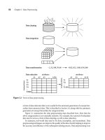
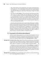
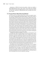
Clustering by pattern similarity in DNA microarray analysis. Figure 7.22 shows a frag-
ment of microarray data containing only three genes (taken as “objects” here) and ten
attributes (columns ato j). No patterns among the three objects are visibly explicit. How-
ever, if two subsets of attributes, {b, c, h, j, e}and {f, d, a, g, i}, are selected and plotted
as in Figure 7.23(a) and (b) respectively, it is easy to see that they form some interest-
ing patterns: Figure 7.23(a) forms a shift pattern, where the three curves are similar to
each other with respect to a shift operation along the y-axis; while Figure 7.23(b) forms a
scaling pattern, where the three curves are similar to each other with respect to a scaling
operation along the y-axis.
Let us first examine how to discover shift patterns. In DNA microarray data, each row
corresponds to a gene and each column or attribute represents a condition under which
the gene is developed. The usual Euclidean distance measure cannot capture pattern
similarity, since the y values of different curves can be quite far apart. Alternatively, we
could first transform the data to derive new attributes, such as A
i j
= v
i
−v
j
(where v
i
and
9
Entropy is a measure from information theory. It was introduced in Chapter 2 regarding data dis-
cretization and is also described in Chapter 6 regarding decision tree construction.
442 Chapter 7 Cluster Analysis
a b c d e f g h i j
90

80
70
60
50
40
30
20
10
0
Object 1
Object 2
Object 3
Figure 7.22 Raw data from a fragment of microarray data containing only 3 objects and 10 attributes.
a
b c
d
e
f g
h
i
j
90
80
70
60
50
40
30
20
10

0
90
80
70
60
50
40
30
20
10
0
Object 1
Object 2
Object 3
Object 1
Object 2
Object 3
(a) (b)
Figure 7.23 Objects in Figure 7.22 form (a) a shift pattern in subspace {b, c, h, j, e}, and (b) a scaling
pattern in subspace {f, d, a, g, i}.
v
j
are object values for attributes A
i
and A
j
, respectively), and then cluster on the derived
attributes. However, this would introduce d(d −1)/2 dimensions for a d-dimensional
data set, which is undesirable for a nontrivial d value. A biclustering method was pro-
posed in an attempt to overcome these difficulties. It introduces a new measure, the mean

7.9 Clustering High-Dimensional Data 443
squared residue score, which measures the coherence of the genes and conditions in a
submatrix of a DNA array. Let I ⊂ X and J ⊂Y be subsets of genes, X, and conditions,
Y, respectively. The pair, (I, J), specifies a submatrix, A
IJ
, with the mean squared residue
score defined as
H(IJ) =
1
|I||J|
∑
i∈I, j∈J
(d
i j
−d
iJ
−d
I j
+ d
IJ
)
2
, (7.39)
where d
i j
is the measured value of gene i for condition j, and
d
iJ
=
1

|J|
∑
j∈J
d
i j
, d
I j
=
1
|I|
∑
i∈I
d
i j
, d
IJ
=
1
|I||J|
∑
i∈I, j∈J
d
i j
, (7.40)
where d
iJ
and d
I j
are the row and column means, respectively, and d
IJ

is the mean of
the subcluster matrix, A
IJ
. A submatrix, A
IJ
, is called a δ-bicluster if H(I, J) ≤ δ for
some δ > 0. A randomized algorithm is designed to find such clusters in a DNA array.
There are two major limitations of this method. First, a submatrix of a δ-bicluster is not
necessarily a δ-bicluster, which makes it difficult to design an efficient pattern growth–
based algorithm. Second, because of the averaging effect, a δ-bicluster may contain some
undesirable outliers yet still satisfy a rather small δ threshold.
To overcome the problems of the biclustering method, a pCluster model was intro-
duced as follows. Given objects x, y ∈ O and attributes a, b ∈ T, pScore is defined by a
2×2 matrix as
pScore(

d
xa
d
xb
d
ya
d
yb

) = |(d
xa
−d
xb
) −(d

ya
−d
yb
)|, (7.41)
where d
xa
is the value of object (or gene) x for attribute (or condition) a, and so on.
A pair, (O, T), forms a δ-pCluster if, for any 2 ×2 matrix, X, in (O, T), we have
pScore(X) ≤ δ for some δ > 0. Intuitively, this means that the change of values on the
two attributes between the two objects is confined by δ for every pair of objects in O and
every pair of attributes in T.
It is easy to see that δ-pCluster has the downward closure property; that is, if (O, T)
forms a δ-pCluster, then any of its submatrices is also a δ-pCluster. Moreover, because
a pCluster requires that every two objects and every two attributes conform with the
inequality, the clusters modeled by the pCluster method are more homogeneous than
those modeled by the bicluster method.
In frequent itemset mining, itemsets are considered frequent ifthey satisfy a minimum
support threshold, which reflects their frequency of occurrence. Based on the definition
of pCluster, the problem of mining pClusters becomes one of mining frequent patterns
in which each pair of objects and their corresponding features must satisfy the specified
δ threshold. A frequent pattern–growth method can easily be extended to mine such
patterns efficiently.
444 Chapter 7 Cluster Analysis
Now, let’s look into how to discover scaling patterns. Notice that the original pScore
definition, though defined for shift patterns in Equation (7.41), can easily be extended
for scaling by introducing a new inequality,
d
xa
/d
ya

d
xb
/d
yb
≤ δ

. (7.42)
This can be computed efficiently because Equation (7.41) is a logarithmic form of
Equation (7.42). That is, the same pCluster model can be applied to the data set after
converting the data to the logarithmic form. Thus, the efficient derivation of δ-pClusters
for shift patterns can naturally be extended for the derivation of δ-pClusters for scaling
patterns.
The pCluster model, though developed in the study of microarray data cluster
analysis, can be applied to many other applications that require finding similar or coher-
ent patterns involving a subset of numerical dimensions in large, high-dimensional
data sets.
7.10
Constraint-Based Cluster Analysis
In the above discussion, we assume that cluster analysis is an automated, algorithmic
computationalprocess,basedon the evaluation of similarity or distancefunctions among
a set of objects to be clustered, with little user guidance or interaction. However,users often
have a clear view of the application requirements, which they would ideally like to use to
guide the clustering process and influence the clustering results. Thus, in many applica-
tions, it is desirable to have the clustering process take user preferences and constraints
into consideration. Examples of such information include the expected number of clus-
ters, the minimal or maximal cluster size, weights for different objects or dimensions,
and other desirable characteristics of the resulting clusters. Moreover, when a clustering
task involves a rather high-dimensional space, it is very difficult to generate meaningful
clusters by relying solely on the clustering parameters. User input regarding important
dimensions or the desired results will serve as crucial hints or meaningful constraints

for effective clustering. In general, we contend that knowledge discovery would be most
effective if one could develop an environment for human-centered, exploratory min-
ing of data, that is, where the human user is allowed to play a key role in the process.
Foremost, a user should be allowed to specify a focus—directing the mining algorithm
toward the kind of “knowledge” that the user is interested in finding. Clearly, user-guided
mining will lead to more desirable results and capture the application semantics.
Constraint-based clustering finds clusters that satisfy user-specified preferences or
constraints. Depending on the nature of the constraints, constraint-based clustering
may adopt rather different approaches. Here are a few categories of constraints.
1. Constraints on individual objects: We can specify constraints on the objects to be
clustered. In a real estate application, for example, one may like to spatially cluster only
7.10 Constraint-Based Cluster Analysis 445
those luxury mansions worth over a million dollars. This constraint confines the set
of objects to be clustered. It can easily be handled by preprocessing (e.g., performing
selection using an SQL query), after which the problem reduces to an instance of
unconstrained clustering.
2. Constraints on the selection of clustering parameters: A user may like to set a desired
range for each clustering parameter. Clustering parameters are usually quite specific
to the given clustering algorithm. Examples of parameters include k, the desired num-
ber of clusters in a k-means algorithm; or ε (the radius) and MinPts (the minimum
number of points) in the DBSCAN algorithm. Although such user-specified param-
eters may strongly influence the clustering results, they are usually confined to the
algorithm itself. Thus, their fine tuning and processing are usually not considered a
form of constraint-based clustering.
3. Constraints on distance or similarity functions: We can specify different distance or
similarity functions for specific attributes of the objects to be clustered, or different
distance measures for specific pairs of objects. When clustering sportsmen, for exam-
ple, we may use different weighting schemes for height, body weight, age, and skill
level. Although this will likely change the mining results, it may not alter the cluster-
ing process per se. However, in some cases, such changes may make the evaluation

of the distance function nontrivial, especially when it is tightly intertwined with the
clustering process. This can be seen in the following example.
Example 7.16
Clustering with obstacle objects. A city may have rivers, bridges, highways, lakes, and
mountains. We do not want to swim across a river to reach an automated banking
machine. Such obstacle objects and their effects can be captured by redefining the
distance functions among objects. Clustering with obstacle objects using a partition-
ing approach requires that the distance between each object and its corresponding
cluster center be reevaluated at each iteration whenever the cluster center is changed.
However, such reevaluation is quite expensive with the existence of obstacles. In this
case, efficient new methods should be developed for clustering with obstacle objects
in large data sets.
4. User-specified constraints on the properties of individual clusters: A user may like to
specify desired characteristics of the resulting clusters, which may strongly influence
the clustering process. Such constraint-based clustering arises naturally in practice,
as in Example 7.17.
Example 7.17
User-constrained cluster analysis. Suppose a package delivery company would like to
determine the locations for k service stations in a city. The company has a database
of customers that registers the customers’ names, locations, length of time since
the customers began using the company’s services, and average monthly charge.
We may formulate this location selection problem as an instance of unconstrained
clustering using a distance function computed based on customer location. How-
ever, a smarter approach is to partition the customers into two classes: high-value
446 Chapter 7 Cluster Analysis
customers (who need frequent, regular service) and ordinary customers (who require
occasional service). In order to save costs and provide good service, the manager
adds the following constraints: (1) each station should serve at least 100 high-value
customers; and (2) each station should serve at least 5,000 ordinary customers.
Constraint-based clustering will take such constraints into consideration during the

clustering process.
5. Semi-supervised clustering based on “partial” supervision: The quality of unsuper-
vised clustering can be significantly improved using some weak form of supervision.
This may be in the form of pairwise constraints (i.e., pairs of objects labeled as belong-
ing to the same or different cluster). Such a constrained clustering process is called
semi-supervised clustering.
In this section, we examine how efficient constraint-based clustering methods can be
developed for large data sets. Since cases 1 and 2 above are trivial, we focus on cases 3 to
5 as typical forms of constraint-based cluster analysis.
7.10.1 Clustering with Obstacle Objects
Example 7.16 introduced the problem of clustering with obstacle objects regarding the
placement of automated banking machines. The machines should be easily accessible to
the bank’s customers. This means that during clustering, we must take obstacle objects
into consideration, such as rivers, highways, and mountains. Obstacles introduce con-
straints on the distance function. The straight-line distance between two points is mean-
ingless if there is an obstacle in the way. As pointed out in Example 7.16, we do not want
to have to swim across a river to get to a banking machine!
“How can we approach the problem of clustering with obstacles?” A partitioning clus-
tering method is preferable because it minimizes the distance between objects and
their cluster centers. If we choose the k-means method, a cluster center may not be
accessible given the presence of obstacles. For example, the cluster mean could turn
out to be in the middle of a lake. On the other hand, the k-medoids method chooses
an object within the cluster as a center and thus guarantees that such a problem can-
not occur. Recall that every time a new medoid is selected, the distance between each
object and its newly selected cluster center has to be recomputed. Because there could
be obstacles between two objects, the distance between two objects may have to be
derived by geometric computations (e.g., involving triangulation). The computational
cost can get very high if a large number of objects and obstacles are involved.
The clustering with obstacles problem can be represented using a graphical nota-
tion. First, a point, p, is visible from another point, q, in the region, R, if the straight

line joining p and q does not intersect any obstacles. A visibility graph is the graph,
VG = (V, E), such that each vertex of the obstacles has a corresponding node in
V and two nodes, v
1
and v
2
, in V are joined by an edge in E if and only if the
corresponding vertices they represent are visible to each other. Let VG

= (V

, E

)
be a visibility graph created from VG by adding two additional points, p and q, in
7.10 Constraint-Based Cluster Analysis 447
V

. E

contains an edge joining two points in V

if the two points are mutually vis-
ible. The shortest path between two points, p and q, will be a subpath of VG

as
shown in Figure 7.24(a). We see that it begins with an edge from p to either v
1
, v
2

,
or v
3
, goes through some path in VG, and then ends with an edge from either v
4
or
v
5
to q.
To reduce the cost of distance computation between any two pairs of objects or
points, several preprocessing and optimization techniques can be used. One method
groups points that are close together into microclusters. This can be done by first
triangulating the region R into triangles, and then grouping nearby points in the
same triangle into microclusters, using a method similar to BIRCH or DBSCAN, as
shown in Figure 7.24(b). By processing microclusters rather than individual points,
the overall computation is reduced. After that, precomputation can be performed
to build two kinds of join indices based on the computation of the shortest paths:
(1) VV indices, for any pair of obstacle vertices, and (2) MV indices, for any pair
of microcluster and obstacle vertex. Use of the indices helps further optimize the
overall performance.
With such precomputation and optimization, the distance between any two points
(at the granularity level of microcluster) can be computed efficiently. Thus, the clus-
tering process can be performed in a manner similar to a typical efficient k-medoids
algorithm, such as CLARANS, and achieve good clustering quality for large data sets.
Given a large set of points, Figure 7.25(a) shows the result of clustering a large set of
points without considering obstacles, whereas Figure 7.25(b) shows the result with con-
sideration of obstacles. The latter represents rather different but more desirable clusters.
For example, if we carefully compare the upper left-hand corner of the two graphs, we
see that Figure 7.25(a) has a cluster center on an obstacle (making the center inaccessi-
ble), whereas all cluster centers in Figure 7.25(b) are accessible. A similar situation has

occurred with respect to the bottom right-hand corner of the graphs.
p
q
VG
VG’
(a) (b)
o
2
o
1
v
1
v
2
v
3
v
4
v
5
Figure 7.24 Clustering with obstacle objects (o
1
and o
2
): (a) a visibility graph, and (b) triangulation of
regions with microclusters. From [THH01].
448 Chapter 7 Cluster Analysis
(a) (b)
Figure 7.25 Clustering results obtained without and with consideration of obstacles (where rivers and
inaccessible highways or city blocks are represented by polygons): (a) clustering without con-

sidering obstacles, and (b) clustering with obstacles.
7.10.2 User-Constrained Cluster Analysis
Let’s examine the problem of relocating package delivery centers, as illustrated in
Example 7.17. Specifically, a package delivery company with n customers would like
to determine locations for k service stations so as to minimize the traveling distance
between customers and service stations. The company’s customers are regarded as
either high-value customers (requiring frequent, regular services) or ordinary customers
(requiring occasional services). The manager has stipulated two constraints: each sta-
tion should serve (1) at least 100 high-value customers and (2) at least 5,000 ordinary
customers.
This can be considered as a constrained optimization problem. We could consider
using a mathematical programming approach to handle it. However, such a solution is
difficult to scale to large data sets. To cluster n customers into k clusters, a mathematical
programming approach will involve at least k ×n variables. As n can be as large as a
few million, we could end up having to solve a few million simultaneous equations—
a very expensive feat. A more efficient approach is proposed that explores the idea of
microclustering, as illustrated below.
The general idea of clustering a large data set into k clusters satisfying user-specified
constraints goes as follows. First, we can find an initial “solution” by partitioning the
data set into k groups, satisfying the user-specified constraints, such as the two con-
straints in our example. We then iteratively refine the solution by moving objects from
one cluster to another, trying to satisfy the constraints. For example, we can move a set
of m customers from cluster C
i
to C
j
if C
i
has at least m surplus customers (under the
specified constraints), or if the result of moving customers into C

i
from some other
clusters (including from C
j
) would result in such a surplus. The movement is desirable
7.10 Constraint-Based Cluster Analysis 449
if the total sum of the distances of the objects to their corresponding cluster centers is
reduced. Such movement can be directed by selecting promising points to be moved,
such as objects that are currently assigned to some cluster, C
i
, but that are actually closer
to a representative (e.g., centroid) of some other cluster, C
j
. We need to watch out for
and handle deadlock situations (where a constraint is impossible to satisfy), in which
case, a deadlock resolution strategy can be employed.
To increase the clustering efficiency, data can first be preprocessed using the micro-
clustering idea to form microclusters (groups of points that are close together), thereby
avoiding the processing of all of the points individually. Object movement, deadlock
detection, and constraint satisfaction can be tested at the microcluster level, which re-
duces the number of points to be computed. Occasionally, such microclusters may need
to be broken up in order to resolve deadlocks under the constraints. This methodol-
ogy ensures that the effective clustering can be performed in large data sets under the
user-specified constraints with good efficiency and scalability.
7.10.3 Semi-Supervised Cluster Analysis
In comparison with supervised learning, clustering lacks guidance from users or classi-
fiers (such as class label information), and thus may not generate highly desirable clus-
ters. The quality of unsupervised clustering can be significantly improved using some
weak form of supervision, for example, in the form of pairwise constraints (i.e., pairs of
objects labeled as belonging to the same or different clusters). Such a clustering process

based on user feedback or guidance constraints is called semi-supervised clustering.
Methods for semi-supervised clustering can be categorized into two classes:
constraint-based semi-supervised clustering and distance-based semi-supervised clustering.
Constraint-based semi-supervised clustering relies on user-provided labels or constraints
to guide the algorithm toward a more appropriate data partitioning. This includes mod-
ifying the objective function based on constraints, or initializing and constraining the
clustering process based on the labeled objects. Distance-based semi-supervised clus-
tering employs an adaptive distance measure that is trained to satisfy the labels or con-
straints in the supervised data. Several different adaptive distance measures have been
used, such as string-edit distance trained using Expectation-Maximization (EM), and
Euclidean distance modified by a shortest distance algorithm.
An interesting clustering method, called CLTree (CLustering based on decision
TREEs), integrates unsupervised clustering with the idea of supervised classification. It
is an example of constraint-based semi-supervised clustering. It transforms a clustering
task into a classification task by viewing the set of points to be clustered as belonging to
one class, labeled as “Y,” and adds a set of relatively uniformly distributed, “nonexistence
points” with a different class label, “N.” The problem of partitioning the data space into
data (dense) regions and empty (sparse) regions can then be transformed into a classifi-
cation problem. For example, Figure 7.26(a) contains a set of data points to be clustered.
These points can be viewed as a set of “Y” points. Figure 7.26(b) shows the addition of
a set of uniformly distributed “N” points, represented by the “◦” points. The original
450 Chapter 7 Cluster Analysis
(a) (b) (c)
Figure 7.26 Clustering through decision tree construction: (a) the set of data points to be clustered,
viewed as a set of “Y” points, (b) the addition of a set of uniformly distributed “N” points,
represented by “◦”, and (c) the clustering result with “Y” points only.
clustering problem is thus transformed into a classification problem, which works out
a scheme that distinguishes “Y” and “N” points. A decision tree induction method can
be applied
10

to partition the two-dimensional space, as shown in Figure 7.26(c). Two
clusters are identified, which are from the “Y” points only.
Adding a large number of “N” points to the original data may introduce unneces-
sary overhead in computation. Furthermore, it is unlikely that any points added would
truly be uniformly distributed in a very high-dimensional space as this would require an
exponential number of points. To deal with this problem, we do not physically add any
of the “N” points, but only assume their existence. This works because the decision tree
method does not actually require the points. Instead, it only needs the number of “N”
points at each decision tree node. This number can be computed when needed, with-
out having to add points to the original data. Thus, CLTree can achieve the results in
Figure 7.26(c) without actually adding any “N” points to the original data. Again, two
clusters are identified.
The question then is how many (virtual) “N” points should be added in order to
achieve good clustering results. The answer follows this simple rule: At the root node, the
number of inherited “N” points is 0. At any current node, E, if the number of “N” points
inherited from the parent node of E is less than the number of “Y” points in E, then the
number of “N” points for E is increased to the number of “Y” points in E. (That is, we set
the number of “N” points to be as big as the number of “Y” points.) Otherwise, the number
of inherited “N” points is used in E. The basic idea is to use an equal number of “N”
points to the number of “Y” points.
Decision tree classification methods use a measure, typically based on information
gain, to select the attribute test for a decision node (Section 6.3.2). The data are then
split or partitioned according the test or “cut.” Unfortunately, with clustering, this can
lead to the fragmentation of some clusters into scattered regions. Toaddress this problem,
methods were developed that use information gain, but allow the ability to look ahead.
10
Decision tree induction was described in Chapter 6 on classification.
7.11 Outlier Analysis 451
That is, CLTree first finds initial cuts and then looks ahead to find better partitions that
cut less into cluster regions. It finds those cuts that form regions with a very low relative

density. The idea is that we want to split at the cut point that may result in a big empty
(“N”) region, which is more likely to separate clusters. With such tuning, CLTree can per-
form high-quality clustering in high-dimensional space. It can also find subspace clusters
as the decision tree method normally selects only a subset of the attributes. An interest-
ing by-product of this method is the empty (sparse) regions, which may also be useful
in certain applications. In marketing, for example, clusters may represent different seg-
ments of existing customers of a company, while empty regions reflect the profiles of
noncustomers. Knowing the profiles of noncustomers allows the company to tailor their
services or marketing to target these potential customers.
7.11
Outlier Analysis
“What is an outlier?” Very often, there exist data objects that do not comply with the
general behavior or model of the data. Such data objects, which are grossly different
from or inconsistent with the remaining set of data, are called outliers.
Outliers can be caused by measurement or execution error. For example, the display
of a person’s age as −999 could be caused by a program default setting of an unrecorded
age. Alternatively, outliers may be the result of inherent data variability. The salary of the
chief executive officer of a company, for instance, could naturally stand out as an outlier
among the salaries of the other employees in the firm.
Many data mining algorithms try to minimize the influence of outliers or eliminate
them all together. This, however, could result in the loss of important hidden information
because one person’s noise could be another person’s signal. In other words, the outliers
may be of particular interest, such as in the case of fraud detection, where outliers may
indicate fraudulent activity. Thus, outlier detection and analysis is an interesting data
mining task, referred to as outlier mining.
Outlier mining has wide applications. As mentioned previously,itcan be used in fraud
detection, for example, by detecting unusual usage of credit cards or telecommunica-
tion services. In addition, it is useful in customized marketing for identifying the spend-
ing behavior of customers with extremely low or extremely high incomes, or in medical
analysis for finding unusual responses to various medical treatments.

Outlier mining can be described as follows: Given a set of n data points or objects
and k, the expected number of outliers, find the top k objects that are considerably
dissimilar, exceptional, or inconsistent with respect to the remaining data. The outlier
mining problem can be viewed as two subproblems: (1) define what data can be
considered as inconsistent in a given data set, and (2) find an efficient method to
mine the outliers so defined.
The problem of defining outliers is nontrivial. If a regression model is used for data
modeling, analysis of the residuals can give a good estimation for data “extremeness.”
The task becomes tricky, however, when finding outliers in time-series data, as they may
be hidden in trend, seasonal, or other cyclic changes. When multidimensional data are
452 Chapter 7 Cluster Analysis
analyzed, not any particular one but rather a combination of dimension values may be
extreme. For nonnumeric (i.e., categorical) data, the definition ofoutliers requires special
consideration.
“What about using data visualization methods for outlier detection?” This may seem like
an obvious choice, since human eyes are very fast and effective at noticing data inconsis-
tencies. However, this does not apply to data containing cyclic plots, where values that
appear to be outliers could be perfectly valid values in reality. Data visualization meth-
ods are weak in detecting outliers in data with many categorical attributes or in data of
high dimensionality, since human eyes are good at visualizing numeric data of only two
to three dimensions.
In this section, we instead examine computer-based methods for outlier detection.
These can be categorized into four approaches: the statistical approach, the distance-based
approach, the density-based local outlier approach, and the deviation-based approach, each
of which are studied here. Notice that while clustering algorithms discard outliers as
noise, they can be modified to include outlier detection as a by-product of their execu-
tion. In general, users must check that each outlier discovered by these approaches is
indeed a “real” outlier.
7.11.1 Statistical Distribution-Based Outlier Detection
The statistical distribution-based approach to outlier detection assumes a distribution

or probability model for the given data set (e.g., a normal or Poisson distribution) and
then identifies outliers with respect to the model using a discordancy test. Application of
the test requires knowledge of the data set parameters (such as the assumed data distri-
bution), knowledge of distribution parameters (such as the mean and variance), and the
expected number of outliers.
“How does the discordancy testing work?” A statistical discordancy test examines two
hypotheses: a working hypothesis and an alternative hypothesis. A working hypothesis,
H, is a statement that the entire data set of n objects comes from an initial distribution
model, F, that is,
H : o
i
∈ F, where i = 1, 2, ., n. (7.43)
The hypothesis is retained if there is no statistically significant evidence supporting its
rejection. A discordancy test verifies whether an object, o
i
, is significantly large (or small)
in relation to the distribution F. Different test statistics have been proposed for use as
a discordancy test, depending on the available knowledge of the data. Assuming that
some statistic, T , has been chosen for discordancy testing, and the value of the statistic for
object o
i
is v
i
, then the distribution of T is constructed. Significance probability, SP(v
i
) =
Prob(T > v
i
), is evaluated. If SP(v
i

) is sufficiently small, then o
i
is discordant and the
working hypothesis is rejected. An alternative hypothesis,
H, which states that o
i
comes
from another distribution model, G, is adopted. The result is very much dependent on
which model F is chosen because o
i
may be an outlier under one model and a perfectly
valid value under another.
7.11 Outlier Analysis 453
The alternative distribution is very important in determining the power of the test,
that is, the probability that the working hypothesis is rejected when o
i
is really an outlier.
There are different kinds of alternative distributions.
Inherent alternative distribution: In this case, the working hypothesis that all of the
objects come from distribution F is rejected in favor of the alternative hypothesis that
all of the objects arise from another distribution, G:
H : o
i
∈ G, where i = 1, 2, ., n. (7.44)
F and G may be different distributions or differ only in parameters of the same dis-
tribution. There are constraints on the form of the G distribution in that it must have
potential to produce outliers. For example, it may have a different mean or dispersion,
or a longer tail.
Mixture alternative distribution: The mixture alternative states that discordant values
are not outliers in the F population, but contaminants from some other population,

G. In this case, the alternative hypothesis is
H : o
i
∈ (1−λ)F +λG, where i = 1, 2, , n. (7.45)
Slippage alternative distribution: This alternative states that all of the objects (apart
from some prescribed small number) arise independently from the initial model, F,
with its given parameters, whereas the remaining objects are independent observa-
tions from a modified version of F in which the parameters have been shifted.
There are two basic types of procedures for detecting outliers:
Block procedures: In this case, either all of the suspect objects are treated as outliers
or all of them are accepted as consistent.
Consecutive (or sequential) procedures: An example of such a procedure is the inside-
out procedure. Its main idea is that the object that is least “likely” to be an outlier is
tested first. If it is found to be an outlier, then all of the more extreme values are also
considered outliers; otherwise, the next most extreme object is tested, and so on. This
procedure tends to be more effective than block procedures.
“How effective is the statistical approach at outlier detection?” A major drawback is that
most tests are for single attributes, yet many data mining problems require finding out-
liers in multidimensional space. Moreover, the statistical approach requires knowledge
about parameters of the data set, such as the data distribution. However, in many cases,
the data distribution may not be known. Statistical methods do not guarantee that all
outliers will be found for the cases where no specific test was developed, or where the
observed distribution cannot be adequately modeled with any standard distribution.
454 Chapter 7 Cluster Analysis
7.11.2 Distance-Based Outlier Detection
The notion of distance-based outliers was introduced to counter the main limitations
imposed by statistical methods. An object, o, in a data set, D, is a distance-based (DB)
outlier with parameters pct and dmin,
11
that is, a DB(pct,dmin)-outlier, if at least a frac-

tion, pct, of the objects in D lie at a distance greater than dmin from o. In other words,
rather than relying on statistical tests, we can think of distance-based outliers as those
objects that do not have “enough” neighbors, where neighbors are defined based on
distance from the given object. In comparison with statistical-based methods, distance-
based outlier detection generalizes the ideas behind discordancy testing for various stan-
dard distributions. Distance-based outlier detection avoids the excessive computation
that can be associated with fitting the observed distribution into some standard distri-
bution and in selecting discordancy tests.
For many discordancy tests, it can be shown that if an object, o, is an outlier according
to the given test, then o is also a DB(pct, dmin)-outlier for some suitably defined pct and
dmin. For example, if objects that lie three or more standard deviations from the mean
are considered to be outliers, assuming a normal distribution, then this definition can
be generalized by a DB(0.9988, 0.13σ) outlier.
12
Several efficient algorithms for mining distance-based outliers have been developed.
These are outlined as follows.
Index-based algorithm: Given a data set, the index-based algorithm uses multidimen-
sional indexing structures, such as R-trees or k-d trees, to search for neighbors of each
object o within radius dmin around that object. Let M be the maximum number of
objects within the dmin-neighborhood of an outlier. Therefore, once M +1 neighbors
of object o are found, it is clear that o is not an outlier. This algorithm has a worst-case
complexity of O(n
2
k), where n is the number of objects in the data set and k is the
dimensionality. The index-based algorithm scales well as k increases. However, this
complexity evaluation takes only the search time into account, even though the task
of building an index in itself can be computationally intensive.
Nested-loop algorithm: The nested-loop algorithm has the same computational com-
plexity as the index-based algorithm but avoids index structure construction and tries
to minimize the number of I/Os. It divides the memory buffer space into two halves

and the data set into several logical blocks. By carefully choosing the order in which
blocks are loaded into each half, I/O efficiency can be achieved.
11
The parameter dmin is the neighborhood radius around object o. It corresponds to the parameter ε
in Section 7.6.1.
12
The parameters pct and dmin are computed using the normal curve’s probability density function to
satisfy the probability condition (P|x−3|≤dmin) < 1−pct, i.e., P(3−dmin ≤x ≤3+dmin) < −pct,
where x is an object. (Note that the solution may not be unique.) A dmin-neighborhood of radius 0.13
indicates a spread of ±0.13 units around the 3 σ mark (i.e., [2.87, 3.13]). For a complete proof of the
derivation, see [KN97].
7.11 Outlier Analysis 455
Cell-based algorithm: To avoid O(n
2
) computationalcomplexity,a cell-based algorithm
was developed for memory-resident data sets. Its complexity is O(c
k
+ n), where c
is a constant depending on the number of cells and k is the dimensionality. In this
method, the data space is partitioned into cells with a side length equal to
dmin
2
√
k
. Each
cell has two layers surrounding it. The first layer is one cell thick, while the second
is 2
√
k −1 cells thick, rounded up to the closest integer. The algorithm counts
outliers on a cell-by-cell rather than an object-by-object basis. For a given cell, it

accumulates three counts—the number of objects in the cell, in the cell and the first
layer together, and in the cell and both layers together. Let’s refer to these counts as
cell
count, cell + 1 layer count, and cell + 2 layers count, respectively.
“How are outliers determined in this method?” Let M be the maximum number of
outliers that can exist in the dmin-neighborhood of an outlier.
An object, o, in the current cell is considered an outlier only if cell + 1 layer count
is less than or equal to M. If this condition does not hold, then all of the objects
in the cell can be removed from further investigation as they cannot be outliers.
If cell + 2 layers count is less than or equal to M, then all of the objects in the
cell are considered outliers. Otherwise, if this number is more than M, then it
is possible that some of the objects in the cell may be outliers. To detect these
outliers, object-by-object processing is used where, for each object, o, in the cell,
objects in the second layer of o are examined. For objects in the cell, only those
objects having no more than M points in their dmin-neighborhoods are outliers.
The dmin-neighborhood of an object consists of the object’s cell, all of its first
layer, and some of its second layer.
A variation to the algorithm is linear with respect to n and guarantees that no more
than three passes over the data set are required. It can be used for large disk-resident
data sets, yet does not scale well for high dimensions.
Distance-based outlier detection requires the user to set both the pct and dmin
parameters. Finding suitable settings for these parameters can involve much trial and
error.
7.11.3 Density-Based Local Outlier Detection
Statistical and distance-based outlier detection both depend on the overall or “global”
distribution of the given set of data points, D. However, data are usually not uniformly
distributed. These methods encounter difficulties when analyzing data with rather dif-
ferent density distributions, as illustrated in the following example.
Example 7.18
Necessity for density-based local outlier detection. Figure 7.27 shows a simple 2-D data

set containing 502 objects, with two obvious clusters. Cluster C
1
contains 400 objects.
Cluster C
2
contains 100 objects. Two additional objects, o
1
and o
2
are clearly outliers.
However, by distance-based outlier detection (which generalizes many notions from
456 Chapter 7 Cluster Analysis
C
2
C
1
o
2
o
1
Figure 7.27 The necessity of density-based local outlier analysis. From [BKNS00].
statistical-based outlier detection), onlyo
1
is a reasonable DB(pct, dmin)-outlier, because
if dmin is set to be less than the minimum distance between o
2
andC
2
, then all 501 objects
are further away from o

2
than dmin. Thus, o
2
would be considered a DB(pct, dmin)-
outlier, but so would all of the objects in C
1
! On the other hand, if dmin is set to be greater
than the minimum distance between o
2
and C
2
, then even when o
2
is not regarded as an
outlier, some points in C
1
may still be considered outliers.
This brings us to the notion of local outliers. An object is a local outlier if it is outlying
relative to its local neighborhood, particulary with respect to the density of the neighbor-
hood. In this view, o
2
of Example 7.18 is a local outlier relative to the density of C
2
.
Object o
1
is an outlier as well, and no objects in C
1
are mislabeled as outliers. This forms
the basis of density-based local outlier detection. Another key idea of this approach to

outlier detection is that, unlike previous methods, it does not consider being an out-
lier as a binary property. Instead, it assesses the degree to which an object is an out-
lier. This degree of “outlierness” is computed as the local outlier factor (LOF) of an
object. It is local in the sense that the degree depends on how isolated the object is with
respect to the surrounding neighborhood. This approach can detect both global and local
outliers.
To define the local outlier factor of an object, we need to introduce the concepts of
k-distance, k-distance neighborhood, reachability distance,
13
and local reachability den-
sity. These are defined as follows:
The k-distance of an object p is the maximal distance that p gets from its k-nearest
neighbors. This distance is denoted as k-distance(p). It is defined as the distance,
d(p, o), between p and an object o ∈D, such that (1) for at least k objects, o

∈ D, it
13
The reachability distance here is similar to the reachability distance defined for OPTICS in
Section 7.6.2, although it is given in a somewhat different context.
7.11 Outlier Analysis 457
holds that d(p, o

) ≤d(p, o). That is, there are at least k objects in D that are as close as
or closer to p than o, and (2) for at most k −1 objects, o

∈D, it holds that d(p, o

) <
d(p, o). That is, there are at most k −1 objects that are closer to p than o. You may be
wondering at this point how k is determined. The LOF method links to density-based

clustering in that it sets k to the parameter MinPts, which specifies the minimum num-
ber of points for use in identifying clusters based on density (Sections 7.6.1 and 7.6.2).
Here, MinPts (as k) is used to define the local neighborhood of an object, p.
The k-distance neighborhood of an object p is denoted N
k
distance(p)
(p), or N
k
(p)
for short. By setting k to MinPts, we get N
MinPts
(p). It contains the MinPts-nearest
neighbors of p. That is, it contains every object whose distance is not greater than the
MinPts-distance of p.
The reachability distance of an object p with respect to object o (where o is within
the MinPts-nearest neighbors of p), is defined as reach
dist
MinPts
(p, o) = max{MinPts-
distance(o), d(p, o)}. Intuitively, if an object p is far away from o, then the reachability
distance between the two is simply their actual distance. However, if they are “suffi-
ciently” close (i.e., where p is within the MinPts-distance neighborhood of o), then
the actual distance is replaced by the MinPts-distance of o. This helps to significantly
reduce the statistical fluctuations of d(p, o) for all of the p close to o. The higher the
value of MinPts is, the more similar is the reachability distance for objects within
the same neighborhood.
Intuitively, the local reachability density of p is the inverse of the average reachability
density based on the MinPts-nearest neighbors of p. It is defined as
lrd
MinPts

(p) =
|N
MinPts
(p)|
Σ
o∈N
MinPts
(p)
reach dist
MinPts
(p, o)
. (7.46)
The local outlier factor (LOF) of p captures the degree to which we call p an outlier.
It is defined as
LOF
MinPts
(p) =
∑
o∈N
MinPts
(p)
lrd
MinPts
(o)
lrd
MinPts
(p)
|N
MinPts
(p)|

. (7.47)
It is the average of the ratio of the local reachability density of p and those of p’s
MinPts-nearest neighbors. It is easy to see that the lower p’s local reachability density
is, and the higher the local reachability density of p’s MinPts-nearest neighbors are,
the higher LOF(p) is.
From this definition, if an object p is not a local outlier, LOF(p) is close to 1. The more
that p is qualified to be a local outlier, the higher LOF(p) is. Therefore, we can determine
whether a point p is a local outlier based on the computation of LOF(p). Experiments
based on both synthetic and real-world large data sets have demonstrated the power of
LOF at identifying local outliers.
458 Chapter 7 Cluster Analysis
7.11.4 Deviation-Based Outlier Detection
Deviation-based outlier detection does not use statistical tests or distance-based
measures to identify exceptional objects. Instead, it identifies outliers by examining the
main characteristics of objects in a group. Objects that “deviate” from this description are
considered outliers. Hence, in this approach the term deviations is typically used to refer
to outliers. In this section, we study two techniques for deviation-based outlier detec-
tion. The first sequentially compares objects in a set, while the second employs an OLAP
data cube approach.
Sequential Exception Technique
The sequential exception technique simulates the way in which humans can distinguish
unusual objects from among a series of supposedly like objects. It uses implicit redun-
dancy of the data. Given a data set, D, of n objects, it builds a sequence of subsets,
{D
1
, D
2
, ., D
m
}, of these objects with 2 ≤m ≤ n such that

D
j−1
⊂ D
j
, where D
j
⊆ D. (7.48)
Dissimilarities are assessed between subsets in the sequence. The technique introduces
the following key terms.
Exception set: This is the set of deviations or outliers. It is defined as the smallest
subset of objects whose removal results in the greatest reduction of dissimilarity in
the residual set.
14
Dissimilarity function: This function does not require a metric distance between the
objects. It is any function that, if given a set of objects, returns a low value if the objects
are similar to one another. The greater the dissimilarity among the objects, the higher
the value returned by the function. The dissimilarity of a subset is incrementally com-
puted based on the subset prior to it in the sequence. Given a subset of n numbers,
{x
1
, ., x
n
}, a possible dissimilarity function is the variance of the numbers in the
set, that is,
1
n
n
∑
i=1
(x

i
−
x)
2
, (7.49)
where x is the mean of the n numbers in the set. For character strings, the dissimilarity
function may be in the form of a pattern string (e.g., containing wildcard characters)
that is used to cover all of the patterns seen so far. The dissimilarity increases when
the pattern covering all of the strings in D
j−1
does not cover any string in D
j
that is
not in D
j−1
.
14
For interested readers, this is equivalent to the greatest reduction in Kolmogorov complexity for the
amount of data discarded.
7.12 Outlier Analysis 459
Cardinality function: This is typically the count of the number of objects in a given set.
Smoothing factor: This function is computed for each subset in the sequence. It
assesses how much the dissimilarity can be reduced by removing the subset from the
original set of objects. This value is scaled by the cardinality of the set. The subset
whose smoothing factor value is the largest is the exception set.
The general task of finding an exception set can be NP-hard (i.e., intractable).
A sequential approach is computationally feasible and can be implemented using a linear
algorithm.
“How does this technique work?” Instead of assessing the dissimilarity of the current
subset with respect to its complementary set, the algorithm selects a sequence of subsets

from the set for analysis. For every subset, it determines the dissimilarity difference of
the subset with respect to the preceding subset in the sequence.
“Can’t the order of the subsets in the sequence affect the results?” To help alleviate any
possible influence of the input order on the results, the above process can be repeated
several times, each with a different random ordering of the subsets. The subset with the
largest smoothing factor value, among all of the iterations, becomes the exception set.
OLAP Data Cube Technique
An OLAP approach to deviation detection uses data cubes to identify regions of anoma-
lies in large multidimensional data. This technique was described in detail in Chapter 4.
For added efficiency, the deviation detection process is overlapped with cube compu-
tation. The approach is a form of discovery-driven exploration, in which precomputed
measures indicating data exceptions are used to guide the user in data analysis, at all lev-
els of aggregation. A cell value in the cube is considered an exception if it is significantly
different from the expected value, based on a statistical model. The method uses visual
cues such as background color to reflect the degree of exception of each cell. The user
can choose to drill down on cells that are flagged as exceptions. The measure value of a
cell may reflect exceptions occurring at more detailed or lower levels of the cube, where
these exceptions are not visible from the current level.
The model considers variations and patterns in the measure value across all of the
dimensions to which a cell belongs. For example, suppose that you have a data cube for
sales data and are viewing the sales summarized per month. With the help of the visual
cues, you notice an increase in sales in December in comparison to all other months.
This may seem like an exception in the time dimension. However, by drilling down on
the month of December to reveal the sales per item in that month, you note that there
is a similar increase in sales for other items during December. Therefore, an increase
in total sales in December is not an exception if the item dimension is considered. The
model considers exceptions hidden at all aggregated group-by’s of a data cube. Manual
detection of such exceptions is difficult because the search space is typically very large,
particularly when there are many dimensions involving concept hierarchies with several
levels.

460 Chapter 7 Cluster Analysis
7.12
Summary
A cluster is a collection of data objects that are similar to one another within the same
cluster and are dissimilar to the objects in other clusters. The process of grouping a
set of physical or abstract objects into classes of similar objects is called clustering.
Cluster analysis has wide applications, including market or customer segmentation,
pattern recognition, biological studies, spatial data analysis, Web document classifi-
cation, and many others. Cluster analysis can be used as a stand-alone data mining
tool to gain insight into the data distribution or can serve as a preprocessing step for
other data mining algorithms operating on the detected clusters.
The quality of clustering can be assessed based on ameasure of dissimilarity of objects,
which can be computed for various types of data, including interval-scaled, binary,
categorical, ordinal, and ratio-scaled variables, or combinations of these variable types.
For nonmetric vector data, the cosine measure and the Tanimoto coefficient are often
used in the assessment of similarity.
Clustering is a dynamic field of research in data mining. Many clustering algorithms
have been developed. These can be categorized into partitioning methods, hierarchical
methods, density-based methods, grid-based methods, model-based methods, methods
for high-dimensional data (including frequent pattern–based methods), and constraint-
based methods. Some algorithms may belong to more than one category.
A partitioning method first creates an initial set of k partitions, where parameter
k is the number of partitions to construct. It then uses an iterative relocation tech-
nique that attempts to improve the partitioning by moving objects from one group
to another. Typical partitioning methods include k-means, k-medoids, CLARANS,
and their improvements.
A hierarchical method creates a hierarchical decomposition of the given set of data
objects. The method can be classified as being either agglomerative (bottom-up) or
divisive (top-down), based on how the hierarchical decomposition is formed. To com-
pensate for the rigidity of merge or split, the quality of hierarchical agglomeration can

be improved by analyzing object linkages at each hierarchical partitioning (such as
in ROCK and Chameleon), or by first performing microclustering (that is, group-
ing objects into “microclusters”) and then operating on the microclusters with other
clustering techniques, such as iterative relocation (as in BIRCH).
A density-based method clusters objects based on the notion of density. It either
grows clusters according to the density of neighborhood objects (such as in DBSCAN)
or according to some density function (such as in DENCLUE). OPTICS is a density-
based method that generates an augmented ordering of the clustering structure of
the data.
A grid-based method first quantizes the object space into a finite number of cells that
form a grid structure, and then performs clustering on the grid structure. STING is
Exercises 461
a typical example of a grid-based method based on statistical information stored in
grid cells. WaveCluster and CLIQUE are two clustering algorithms that are both grid-
based and density-based.
A model-based method hypothesizes a model for each of the clusters and finds the
best fit of the data to that model. Examples of model-based clustering include the
EM algorithm (which uses a mixture density model), conceptual clustering (such
as COBWEB), and neural network approaches (such as self-organizing feature
maps).
Clustering high-dimensional data is of crucial importance, because in many
advanced applications, data objects such as text documents and microarray data
are high-dimensional in nature. There are three typical methods to handle high-
dimensional data sets: dimension-growth subspace clustering, represented by CLIQUE,
dimension-reduction projected clustering, represented by PROCLUS, and frequent
pattern–based clustering, represented by pCluster.
A constraint-based clustering method groups objects based on application-
dependent or user-specified constraints. For example, clustering with the existence of
obstacle objects and clustering under user-specified constraints are typical methods of
constraint-based clustering. Typical examples include clustering with the existence

of obstacle objects, clustering under user-specified constraints, and semi-supervised
clustering based on “weak” supervision (such as pairs of objects labeled as belonging
to the same or different cluster).
One person’s noise could be another person’s signal. Outlier detection and analysis are
very useful for fraud detection, customized marketing, medical analysis, and many
other tasks. Computer-based outlier analysis methods typically follow either a statisti-
cal distribution-based approach, a distance-based approach, a density-based local outlier
detection approach, or a deviation-based approach.
Exercises
7.1 Briefly outline how to compute the dissimilarity between objects described by the
following types of variables:
(a) Numerical (interval-scaled) variables
(b) Asymmetric binary variables
(c) Categorical variables
(d) Ratio-scaled variables
(e) Nonmetric vector objects
7.2 Given the following measurements for the variable age:
18, 22, 25, 42, 28, 43, 33, 35, 56, 28,
462 Chapter 7 Cluster Analysis
standardize the variable by the following:
(a) Compute the mean absolute deviation of age.
(b) Compute the z-score for the first four measurements.
7.3 Given two objects represented by the tuples (22, 1, 42, 10) and (20, 0, 36, 8):
(a) Compute the Euclidean distance between the two objects.
(b) Compute the Manhattan distance between the two objects.
(c) Compute the Minkowski distance between the two objects, using q = 3.
7.4 Section 7.2.3 gave a method wherein a categorical variable having M states can be encoded
by M asymmetric binary variables. Propose a more efficient encoding scheme and state
why it is more efficient.
7.5 Briefly describe the following approaches to clustering: partitioning methods, hierarchical

methods, density-based methods, grid-based methods, model-based methods, methods
for high-dimensional data, and constraint-based methods. Give examples in each case.
7.6 Suppose that the data mining task is to cluster the following eight points (with (x, y)
representing location) into three clusters:
A
1
(2, 10), A
2
(2, 5), A
3
(8, 4), B
1
(5, 8), B
2
(7, 5), B
3
(6, 4), C
1
(1, 2), C
2
(4, 9).
The distance function is Euclidean distance. Suppose initially we assign A
1
, B
1
, and C
1
as the center of each cluster, respectively. Use the k-means algorithm to show only
(a) The three cluster centers after the first round execution
(b) The final three clusters

7.7 Both k-means and k-medoids algorithms can perform effective clustering. Illustrate the
strength and weakness of k-means in comparison with the k-medoids algorithm. Also,
illustrate the strength and weakness of these schemes in comparison with a hierarchical
clustering scheme (such as AGNES).
7.8 Use a diagram to illustrate how, for a constant MinPts value, density-based clusters with
respect to a higher density (i.e., a lower value for ε, the neighborhood radius) are com-
pletely contained in density-connected sets obtained with respect to a lower density.
7.9 Why is it that BIRCH encounters difficulties in finding clusters of arbitrary shape but
OPTICS does not? Can you propose some modifications to BIRCH to help it find clusters
of arbitrary shape?
7.10 Present conditions under which density-based clustering is more suitable than
partitioning-based clustering and hierarchical clustering. Given some application exam-
ples to support your argument.
7.11 Give an example of how specific clustering methods may be integrated, for example,
where one clustering algorithm is used as a preprocessing step for another. In
Exercises 463
addition, provide reasoning on why the integration of two methods may sometimes lead
to improved clustering quality and efficiency.
7.12 Clustering has been popularly recognized as an important data mining task with broad
applications. Give one application example for each of the following cases:
(a) An application that takes clustering as a major data mining function
(b) An application that takes clustering as a preprocessing tool for data preparation for
other data mining tasks
7.13 Data cubes and multidimensional databases contain categorical, ordinal, and numerical
data in hierarchical oraggregateforms. Based on what you have learned about the cluster-
ing methods, design a clustering method that finds clusters in large data cubes effectively
and efficiently.
7.14 Subspace clustering is a methodology for finding interesting clusters in high-dimensional
space. This methodology can be applied to cluster any kind of data. Outline an efficient
algorithm that may extend density connectivity-based clustering for finding clusters of

arbitrary shapes in projected dimensions in a high-dimensional data set.
7.15 [Contributed by Alex Kotov] Describe each of the following clustering algorithms in terms
of the following criteria: (i) shapes of clusters that can be determined; (ii) input para-
meters that must be specified; and (iii) limitations.
(a) k-means
(b) k-medoids
(c) CLARA
(d) BIRCH
(e) ROCK
(f) Chameleon
(g) DBSCAN
7.16 [Contributed by Tao Cheng] Many clustering algorithms handle either only numerical
data, such as BIRCH, or only categorical data, such as ROCK, but not both. Analyze why
this is the case. Note, however, that the EM clustering algorithm can easily be extended
to handle data with both numerical and categorical attributes. Briefly explain why it can
do so and how.
7.17 Human eyes are fast and effective at judging the quality of clustering methods for two-
dimensional data. Can you design a data visualization method that may help humans
visualize data clusters and judge the clustering quality for three-dimensional data? What
about for even higher-dimensional data?
7.18 Suppose that you are to allocate a number of automatic teller machines (ATMs) in a
given region so as to satisfy a number of constraints. Households or places of work
may be clustered so that typically one ATM is assigned per cluster. The clustering, how-
ever, may be constrained by two factors: (1) obstacle objects (i.e., there are bridges,
464 Chapter 7 Cluster Analysis
rivers, and highways that can affect ATM accessibility), and (2) additional user-specified
constraints, such as each ATM should serve at least 10,000 households. How can a cluster-
ing algorithm such as k-means be modified for quality clustering under both constraints?
7.19 For constraint-based clustering, aside from having the minimum number of customers
in each cluster (for ATM allocation) as a constraint, there could be many other kinds of

constraints. For example, a constraint could be in the form of the maximum number
of customers per cluster, average income of customers per cluster, maximum distance
between every two clusters, and so on. Categorize the kinds of constraints that can be
imposed on the clusters produced and discuss how to perform clustering efficiently under
such kinds of constraints.
7.20 Design a privacy-preserving clustering method so that a data owner would be able to
ask a third party to mine the data for quality clustering without worrying about the
potential inappropriate disclosure of certain private or sensitive information stored
in the data.
7.21 Why is outlier mining important? Briefly describe the different approaches behind
statistical-based outlier detection, distanced-based outlier detection, density-based local out-
lier detection, and deviation-based outlier detection.
7.22 Local outlier factor (LOF) is an interesting notion for the discovery of local outliers
in an environment where data objects are distributed rather unevenly. However, its
performance should be further improved in order to efficiently discover local outliers.
Can you propose an efficient method for effective discovery of local outliers in large
data sets?
Bibliographic Notes
Clustering has been studied extensively for more then 40 years and across many disci-
plines due to its broad applications. Most books on pattern classification and machine
learning contain chapters on cluster analysis or unsupervised learning. Several textbooks
are dedicated to the methods of cluster analysis, including Hartigan [Har75], Jain and
Dubes [JD88], Kaufman and Rousseeuw [KR90], and Arabie, Hubert, and De Sorte
[AHS96]. There are also many survey articles on different aspects of clustering meth-
ods. Recent ones include Jain, Murty, and Flynn [JMF99] and Parsons, Haque, and Liu
[PHL04].
Methods for combining variables of different types into a single dissimilarity matrix
were introduced by Kaufman and Rousseeuw [KR90].
For partitioning methods, the k-means algorithm was first introduced by
Lloyd [Llo57] and then MacQueen [Mac67]. The k-medoids algorithms of PAM and

CLARA were proposed by Kaufman and Rousseeuw [KR90]. The k-modes (for clustering
categorical data) and k-prototypes (for clustering hybrid data) algorithms were proposed
by Huang [Hua98]. The k-modes clustering algorithm was also proposed independently
by Chaturvedi, Green, and Carroll [CGC94, CGC01].