Database systems concepts 4th edition phần 6 doc

Silberschatz−Korth−Sudarshan:

Database System
Concepts, Fourth Edition
IV. Data Storage and
Querying
12. Indexing and Hashing
457
© The McGraw−Hill
Companies, 2001
456 Chapter 12 Indexing and Hashing
Perryridge
Perryridge Redwood Round Hill
Brighton Downtown Mianus
Figure 12.9 B
+
-tree for account file with n =5.
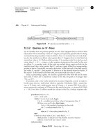
12.3.2 Queries on B
+
-Trees
Let us consider how we process queries on a B
+
-tree. Suppose that we wish to find
all records with a search-key value of V. Figure 12.10 presents pseudocode for doing
so. Intuitively, the procedure works as follows. First, we examine the root node, look-
ing for the smallest search-key value greater than V. Suppose that we find that this
search-key value is K
i
. We then follow pointer P
i
to another node. If we find no such

value, then k ≥ K
m−1
,wherem is the number of pointers in the node. In this case
we follow P
m
to another node. In the node we reached above, again we look for the
smallest search-key value greater than V, and once again follow the corresponding
pointer as above. Eventually, we reach a leaf node. At the leaf node, if we find search-
key value K
i
equals V , then pointer P
i
directs us to the desired record or bucket. If
the value V is not found in the leaf node, no record with key value V exists.
Thus, in processing a query, we traverse a path in the tree from the root to some
leaf node. If there are K search-key values in the file, the path is no longer than
log
n/2
(K).
In practice, only a few nodes need to be accessed, Typically, a node is made to
be the same size as a disk block, which is typically 4 kilobytes. With a search-key
size of 12 bytes, and a disk-pointer size of 8 bytes, n is around 200. Even with a
more conservative estimate of 32 bytes for the search-key size, n is around 100. With
n = 100, if we have 1 million search-key values in the file, a lookup requires only
procedure find(value V )
set C = root node
while C is not a leaf node begin
Let K
i
= smallest search-key value, if any, greater than V

if there is no such value then begin
Let m = the number of pointers in the node
set C = node pointed to by P
m
end
else set C = the node pointed to by P
i
end
if there is a key value K
i
in C such that K
i
= V
then pointer P
i
directs us to the desired record or bucket
else no record with key value k exists
end procedure
Figure 12.10 Querying a B
+
-tree.
Silberschatz−Korth−Sudarshan:

Database System
Concepts, Fourth Edition
IV. Data Storage and
Querying
12. Indexing and Hashing
458
© The McGraw−Hill

Companies, 2001
12.3 B
+
-Tree Index Files 457
log
50
(1,000,000) =4nodes to be accessed. Thus, at most four blocks need to be
read from disk for the lookup. The root node of the tree is usually heavily accessed
and is likely to be in the buffer, so typically only three or fewer blocks need to be read
from disk.
An important difference between B
+
-tree structures and in-memory tree struc-
tures, such as binary trees, is the size of a node, and as a result, the height of the
tree. In a binary tree, each node is small, and has at most two pointers. In a B
+
-tree,
each node is large—typically a disk block—and a node can have a large number of
pointers. Thus, B
+
-trees tend to be fat and short, unlike thin and tall binary trees. In
a balanced binary tree, the path for a lookup can be of length log
2
(K),whereK is
the number of search-key values. With K =1,000,000 as in the previous example, a
balanced binary tree requires around 20 node accesses. If each node were on a differ-
ent disk block, 20 block reads would be required to process a lookup, in contrast to
the four block reads for the B
+
-tree.

12.3.3 Updates on B
+
-Trees
Insertion and deletion are more complicated than lookup, since it may be necessary to
split a node that becomes too large as the result of an insertion, or to coalesce nodes
(that is, combine nodes) if a node becomes too small (fewer than  n/2 pointers).
Furthermore, when a node is split or a pair of nodes is combined, we must ensure
that balance is preserved. To introduce the idea behind insertion and deletion in a
B
+
-tree, we shall assume temporarily that nodes never become too large or too small.
Under this assumption, insertion and deletion are performed as defined next.
• Insertion. Using the same technique as for lookup, we find the leaf node in
which the search-key value would appear. If the search-key value already ap-
pears in the leaf node, we add the new record to the file and, if necessary, add
to the bucket a pointer to the record. If the search-key value does not appear,
we insert the value in the leaf node, and position it such that the search keys
are still in order. We then insert the new record in the file and, if necessary,
create a new bucket with the appropriate pointer.
• Deletion. Using the same technique as for lookup, we find the record to be
deleted, and remove it from the file. We remove the search-key value from the
leaf node if there is no bucket associated with that search-key value or if the
bucket becomes empty as a result of the deletion.
We now consider an example in which a node must be split. Assume that we wish
to insert a record with a branch-name value of “Clearview” into the B
+
-tree of Fig-
ure 12.8. Using the algorithm for lookup, we find that “Clearview” should appear
in the node containing “Brighton” and “Downtown.” There is no room to insert the
search-key value “Clearview.” Therefore, the node is split into two nodes. Figure 12.11

shows the two leaf nodes that result from inserting “Clearview” and splitting the
node containing “Brighton” and “Downtown.” In general, we take the n search-key
Silberschatz−Korth−Sudarshan:

Database System
Concepts, Fourth Edition
IV. Data Storage and
Querying
12. Indexing and Hashing
459
© The McGraw−Hill
Companies, 2001
458 Chapter 12 Indexing and Hashing
Brighton Clearview
Downtown
Figure 12.11 Split of leaf node on insertion of “Clearview.”
values (the n − 1 values in the leaf node plus the value being inserted), and put the
first n/2 in the existing node and the remaining values in a new node.
Having split a leaf node, we must insert the new leaf node into the B
+
-tree struc-
ture. In our example, the new node has “Downtown” as its smallest search-key value.
We need to insert this search-key value into the parent of the leaf node that was split.
The B
+
-tree of Figure 12.12 shows the result of the insertion. The search-key value
“Downtown” was inserted into the parent. It was possible to perform this insertion
because there was room for an added search-key value. If there were no room, the
parent would have had to be split. In the worst case, all nodes along the path to the
root must be split. If the root itself is split, the entire tree becomes deeper.

The general technique for insertion into a B
+
-tree is to determine the leaf node l
into which insertion must occur. If a split results, insert the new node into the parent
of node l. If this insertion causes a split, proceed recursively up the tree until either
an insertion does not cause a split or a new root is created.
Figure 12.13 outlines the insertion algorithm in pseudocode. In the pseudocode,
L.K
i
and L.P
i
denote the ith value and the ith pointer in node L, respectively. The
pseudocode also makes use of the function parent (L) to find the parent of a node L.
We can compute a list of nodes in the path from the root to the leaf while initially
finding the leaf node, and can use it later to find the parent of any node in the path
efficiently. The pseudocode refers to inserting an entry (V,P) into a node. In the case
of leaf nodes, the pointer to an entry actually precedes the key value, so the leaf node
actually stores P before V .Forinternalnodes,P is stored just after V .
We now consider deletions that cause tree nodes to contain too few pointers. First,
let us delete “Downtown” from the B
+
-tree of Figure 12.12. We locate the entry for
“Downtown” by using our lookup algorithm. When we delete the entry for “Down-
town” from its leaf node, the leaf becomes empty. Since, in our example, n =3and
0 < (n −1)/2, this node must be eliminated from the B
+
-tree. To delete a leaf node,
Perryridge
Downtown Mianus
Redwood

Redwood Round Hill
Mianus
Downtown
Brighton Clearview Perryridge
Figure 12.12 Insertion of “Clearview” into the B
+
-tree of Figure 12.8.
Silberschatz−Korth−Sudarshan:

Database System
Concepts, Fourth Edition
IV. Data Storage and
Querying
12. Indexing and Hashing
460
© The McGraw−Hill
Companies, 2001
12.3 B
+
-Tree Index Files 459
procedure insert(value V , pointer P)
find the leaf node L that should contain value V
insert
entry(L, V , P )
end procedure
procedure insert
entry(node L, value V , pointer P)
if (L has space for (V,P))
then insert (V,P) in L
else begin /* Split L */

Create node L

Let V

be the value in L.K
1
, ,L.K
n−1
,V such that exactly
n/2 of the values L.K
1
, ,L.K
n−1
,V are less than V

Let m be the lowest value such that L.K
m
≥ V

/* Note: V

must be either L.K
m
or V */
if (L is a leaf) then begin
move L.P
m
,L.K
m
, ,L.P

n−1
,L.K
n−1
to L

if (V<V

) then insert (P, V ) in L
else insert (P, V ) in L

end
else begin
if (V = V

)/*V is smallest value to go to L

*/
then add P, L.K
m
, ,L.P
n−1
,L.K
n−1
,L.P
n
to L

else add L.P
m
, ,L.P

n−1
,L.K
n−1
,L.P
n
to L

delete L.K
m
, ,L.P
n−1
,L.K
n−1
,L.P
n
from L
if (V<V

) then insert (V,P) in L
else if (V>V

) then insert (V,P) in L

/* Case of V = V

handled already */
end
if (L is not the root of the tree)
then insert
entry(parent (L), V


, L

);
else begin
create a new node R with child nodes L and L

and
the single value V

make R the root of the tree
end
if (L)isaleafnodethen begin /* Fix next child pointers */
set L

.P
n
= L.P
n
;
set L.P
n
= L

end
end
end procedure
Figure 12.13 Insertion of entry in a B
+
-tree.

Silberschatz−Korth−Sudarshan:

Database System
Concepts, Fourth Edition
IV. Data Storage and
Querying
12. Indexing and Hashing
461
© The McGraw−Hill
Companies, 2001
460 Chapter 12 Indexing and Hashing
Perryridge
Mianus
Redwood
Redwood Round Hill
Perryridge
Mianus
Brighton Clearview
Figure 12.14 Deletion of “Downtown” from the B
+
-tree of Figure 12.12.
we must delete the pointer to it from its parent. In our example, this deletion leaves
the parent node, which formerly contained three pointers, with only two pointers.
Since 2 ≥n/2, the node is still sufficiently large, and the deletion operation is
complete. The resulting B
+
-tree appears in Figure 12.14.
When we make a deletion from a parent of a leaf node, the parent node itself may
become too small. That is exactly what happens if we delete “Perryridge” from the
B

+
-tree of Figure 12.14. Deletion of the Perryridge entry causes a leaf node to become
empty. When we delete the pointer to this node in the latter’s parent, the parent is left
with only one pointer. Since n =3, n/2 =2, and thus only one pointer is too few.
However, since the parent node contains useful information, we cannot simply delete
it. Instead, we look at the sibling node (the nonleaf node containing the one search
key, Mianus). This sibling node has room to accommodate the information contained
in our now-too-small node, so we coalesce these nodes, such that the sibling node
now contains the keys “Mianus” and “Redwood.” The other node (the node contain-
ing only the search key “Redwood”) now contains redundant information and can be
deleted from its parent (which happens to be the root in our example). Figure 12.15
shows the result. Notice that the root has only one child pointer after the deletion, so
it is deleted and its sole child becomes the root. So the depth of the B
+
-tree has been
decreased by 1.
It is not always possible to coalesce nodes. As an illustration, delete “Perryridge”
from the B
+
-tree of Figure 12.12. In this example, the “Downtown” entry is still part
ofthetree.Onceagain,theleafnodecontaining“Perryridge” becomes empty. The
parent of the leaf node becomes too small (only one pointer). However, in this ex-
ample, the sibling node already contains the maximum number of pointers: three.
Thus, it cannot accommodate an additional pointer. The solution in this case is to re-
distribute the pointers such that each sibling has two pointers. The result appears in
Mianus Redwood
Redwood Round Hill
Mianus
Brighton Clearview
Figure 12.15 Deletion of “Perryridge” from the B

+
-tree of Figure 12.14.
Silberschatz−Korth−Sudarshan:

Database System
Concepts, Fourth Edition
IV. Data Storage and
Querying
12. Indexing and Hashing
462
© The McGraw−Hill
Companies, 2001
12.3 B
+
-Tree Index Files 461
Mianus
Downtown
Redwood
Redwood Round Hill
Mianus
Downtown
Brighton Clearview
Figure 12.16 Deletion of “Perryridge” from the B
+
-tree of Figure 12.12.
Figure 12.16. Note that the redistribution of values necessitates a change of a search-
key value in the parent of the two siblings.
In general, to delete a value in a B
+
-tree, we perform a lookup on the value and

delete it. If the node is too small, we delete it from its parent. This deletion results
in recursive application of the deletion algorithm until the root is reached, a parent
remains adequately full after deletion, or redistribution is applied.
Figure 12.17 outlines the pseudocode for deletion from a B
+
-tree. The procedure
swap
variables(L, L

) merely swaps the values of the (pointer) variables L and L

;
this swap has no effect on the tree itself. The pseudocode uses the condition “too few
pointers/values.” For nonleaf nodes, this criterion means less than n/2 pointers;
for leaf nodes, it means less than (n − 1)/2 values. The pseudocode redistributes
entries by borrowing a single entry from an adjacent node. We can also redistribute
entries by repartitioning entries equally between the two nodes. The pseudocode
refers to deleting an entry (V,P) from a node. In the case of leaf nodes, the pointer to
an entry actually precedes the key value, so the pointer P precedes the key value V .
For internal nodes, P follows the key value V .
It is worth noting that, as a result of deletion, a key value that is present in an
internal node of the B
+
-tree may not be present at any leaf of the tree.
Although insertion and deletion operations on B
+
-trees are complicated, they re-
quire relatively few
I/O operations, which is an important benefit since I/O opera-
tions are expensive. It can be shown that the number of

I/O operations needed for a
worst-case insertion or deletion is proportional to log
n/2
(K),wheren is the max-
imum number of pointers in a node, and K is the number of search-key values. In
other words, the cost of insertion and deletion operations is proportional to the height
of the B
+
-tree, and is therefore low. It is the speed of operation on B
+
-trees that makes
them a frequently used index structure in database implementations.
12.3.4 B
+
-Tree File Organization
As mentioned in Section 12.3, the main drawback of index-sequential file organiza-
tion is the degradation of performance as the file grows: With growth, an increasing
percentage of index records and actual records become out of order, and are stored in
overflow blocks. We solve the degradation of index lookups by using B
+
-tree indices
on the file. We solve the degradation problem for storing the actual records by using
the leaf level of the B
+
-tree to organize the blocks containing the actual records. We
Silberschatz−Korth−Sudarshan:

Database System
Concepts, Fourth Edition
IV. Data Storage and

Querying
12. Indexing and Hashing
463
© The McGraw−Hill
Companies, 2001
462 Chapter 12 Indexing and Hashing
procedure delete(value V , pointer P)
find the leaf node L that contains (V, P)
delete
entry(L, V, P)
end procedure
procedure delete
entry(node L, value V , pointer P)
delete (V,P) from L
if (L is the root and L has only one remaining child)
then make the child of L the new root of the tree and delete L
else if (L has too few values/pointers) then begin
Let L

be the previous or next child of parent (L)
Let V

be the value between pointers L and L

in parent (L)
if (entries in L and L

can fit in a single node)
then begin /* Coalesce nodes */
if (L is a predecessor of L


) then swap variables(L, L

)
if (L is not a leaf)
then append V

and all pointers and values in L to L

else append all (K
i
,P
i
) pairs in L to L

;setL

.P
n
= L.P
n
delete entry(parent (L), V

, L); delete node L
end
else begin /* Redistribution: borrow an entry from L

*/
if (L


is a predecessor of L) then begin
if (L is a non-leaf node) then begin
let m be such that L

.P
m
is the last pointer in L

remove (L

.K
m−1
,L

.P
m
) from L

insert (L

.P
m
,V

) as the first pointer and value in L,
by shifting other pointers and values right
replace V

in parent (L) by L


.K
m−1
end
else begin
let m be such that (L

.P
m
,L

.K
m
) is the last pointer/value
pair in L

remove (L

.P
m
,L

.K
m
) from L

insert (L

.P
m
,L


.K
m
) as the first pointer and value in L,
by shifting other pointers and values right
replace V

in parent (L) by L

.K
m
end
end
else symmetric to the then case
end
end
end procedure
Figure 12.17 Deletion of entry from a B
+
-tree.
Silberschatz−Korth−Sudarshan:

Database System
Concepts, Fourth Edition
IV. Data Storage and
Querying
12. Indexing and Hashing
464
© The McGraw−Hill
Companies, 2001

12.3 B
+
-Tree Index Files 463
use the B
+
-tree structure not only as an index, but also as an organizer for records in
afile.InaB
+
-tree file organization, the leaf nodes of the tree store records, instead of
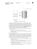
storing pointers to records. Figure 12.18 shows an example of a B
+
-tree file organiza-
tion. Since records are usually larger than pointers, the maximum number of records
that can be stored in a leaf node is less than the number of pointers in a nonleaf node.
However, the leaf nodes are still required to be at least half full.
Insertion and deletion of records from a B
+
-tree file organization are handled in
the same way as insertion and deletion of entries in a B
+
-tree index. When a record
with a given key value v is inserted, the system locates the block that should contain
the record by searching the B
+
-tree for the largest key in the tree that is ≤ v.Ifthe
block located has enough free space for the record, the system stores the record in the
block. Otherwise, as in B
+
-tree insertion, the system splits the block in two, and redis-
tributes the records in it (in the B

+
-tree–key order) to create space for the new record.
The split propagates up the B
+
-tree in the normal fashion. When we delete a record,
the system first removes it from the block containing it. If a block B becomes less
than half full as a result, the records in B are redistributed with the records in an ad-
jacent block B

. Assuming fixed-sized records, each block will hold at least one-half
as many records as the maximum that it can hold. The system updates the nonleaf
nodes of the B
+
-tree in the usual fashion.
When we use a B
+
-tree for file organization, space utilization is particularly im-
portant, since the space occupied by the records is likely to be much more than the
space occupied by keys and pointers. We can improve the utilization of space in a B
+
-
tree by involving more sibling nodes in redistribution during splits and merges. The
technique is applicable to both leaf nodes and internal nodes, and works as follows.
During insertion, if a node is full the system attempts to redistribute some of its
entries to one of the adjacent nodes, to make space for a new entry. If this attempt fails
because the adjacent nodes are themselves full, the system splits the node, and splits
the entries evenly among one of the adjacent nodes and the two nodes that it obtained
by splitting the original node. Since the three nodes together contain one more record
than can fit in two nodes, each node will be about two-thirds full. More precisely, each
node will have at least 2n/3entries, where n is the maximum number of entries that

the node can hold. (xdenotes the greatest integer that is less than or equal to x;that
is, we drop the fractional part, if any.)
C F
K M
I
(A,4) (B,8) (C,1) (D,9) (E,4) (F,7) (G,3) (H,3)
(I,4) (J,8) (K,1) (L,6) (M,4) (N,8) (P,6)
Figure 12.18 B
+
-tree file organization.
Silberschatz−Korth−Sudarshan:

Database System
Concepts, Fourth Edition
IV. Data Storage and
Querying
12. Indexing and Hashing
465
© The McGraw−Hill
Companies, 2001
464 Chapter 12 Indexing and Hashing
During deletion of a record, if the occupancy of a node falls below 2n/3,the
system attempts to borrow an entry from one of the sibling nodes. If both sibling
nodes have  2n/3 records, instead of borrowing an entry, the system redistributes
the entries in the node and in the two siblings evenly between two of the nodes, and
deletes the third node. We can use this approach because the total number of entries
is 32n/3−1, which is less than 2n. With three adjacent nodes used for redistribution,
each node can be guaranteed to have 3n/4 entries. In general, if m nodes (m − 1
siblings) are involved in redistribution, each node can be guaranteed to contain at
least (m − 1)n/m entries. However, the cost of update becomes higher as more

sibling nodes are involved in the redistribution.
12.4 B-Tree Index Files
B-tree indices are similar to B
+
-tree indices. The primary distinction between the two
approaches is that a B-tree eliminates the redundant storage of search-key values.
In the B
+
-tree of Figure 12.12, the search keys “Downtown,”“Mianus,”“Redwood,”
and “Perryridge” appear twice. Every search-key value appears in some leaf node;
several are repeated in nonleaf nodes.
A B-tree allows search-key values to appear only once. Figure 12.19 shows a B-tree
that represents the same search keys as the B
+
-tree of Figure 12.12. Since search keys
arenotrepeatedintheB-tree,wemaybeabletostoretheindexinfewertreenodes
than in the corresponding B
+
-tree index. However, since search keys that appear in
nonleaf nodes appear nowhere else in the B-tree, we are forced to include an addi-
tional pointer field for each search key in a nonleaf node. These additional pointers
point to either file records or buckets for the associated search key.
A generalized B-tree leaf node appears in Figure 12.20a; a nonleaf node appears
in Figure 12.20b. Leaf nodes are the same as in B
+
-trees. In nonleaf nodes, the point-
ers P
i
are the tree pointers that we used also for B
+

-trees, while the pointers B
i
are
bucket or file-record pointers. In the generalized B-tree in the figure, there are n − 1
keys in the leaf node, but there are m − 1 keys in the nonleaf node. This discrepancy
occurs because nonleaf nodes must include pointers B
i
, thus reducing the number of
Downtown Redwood
Round Hill
Mianus Perryridge
Brighton Clearview
Downtown
bucket
Redwood
bucket
Brighton
bucket
Clearview
bucket
Mianus
bucket
Perryridge
bucket
Round Hill
bucket
Figure 12.19 B-tree equivalent of B
+
-tree in Figure 12.12.
Silberschatz−Korth−Sudarshan:

Database System
Concepts, Fourth Edition
IV. Data Storage and
Querying
12. Indexing and Hashing
466
© The McGraw−Hill
Companies, 2001
12.5 Static Hashing 465
P
1
K
1
P
2
. . .

P
n−1
K
n−1
P
n
(a)
P
1
B
1
K

1
P
2
B
2
K
2
. . .

P
m−1
B
m−1
K
m−1
P
m
(b)
Figure 12.20 Typical nodes of a B-tree. (a) Leaf node. (b) Nonleaf node.
search keys that can be held in these nodes. Clearly, m<n, but the exact relationship
between m and n depends on the relative size of search keys and pointers.
The number of nodes accessed in a lookup in a B-tree depends on where the search
key is located. A lookup on a B
+
-tree requires traversal of a path from the root of the
tree to some leaf node. In contrast, it is sometimes possible to find the desired value
in a B-tree before reaching a leaf node. However, roughly n timesasmanykeysare
stored in the leaf level of a B-tree as in the nonleaf levels, and, since n is typically
large, the benefit of finding certain values early is relatively small. Moreover, the fact
that fewer search keys appear in a nonleaf B-tree node, compared to B

+
-trees, implies
that a B-tree has a smaller fanout and therefore may have depth greater than that of
the corresponding B
+
-tree. Thus, lookup in a B-tree is faster for some search keys
but slower for others, although, in general, lookup time is still proportional to the
logarithm of the number of search keys.
Deletion in a B-tree is more complicated. In a B
+
-tree, the deleted entry always
appears in a leaf. In a B-tree, the deleted entry may appear in a nonleaf node. The
proper value must be selected as a replacement from the subtree of the node contain-
ing the deleted entry. Specifically, if search key K
i
is deleted, the smallest search key
appearing in the subtree of pointer P
i +1
must be moved to the field formerly occu-
pied by K
i
. Further actions need to be taken if the leaf node now has too few entries.
In contrast, insertion in a B-tree is only slightly more complicated than is insertion in
aB
+
-tree.
The space advantages of B-trees are marginal for large indices, and usually do not
outweigh the disadvantages that we have noted. Thus, many database system imple-
menters prefer the structural simplicity of a B
+

-tree. The exercises explore details of
the insertion and deletion algorithms for B-trees.
12.5 Static Hashing
One disadvantage of sequential file organization is that we must access an index
structure to locate data, or must use binary search, and that results in more
I/O op-
erations. File organizations based on the technique of hashing allow us to avoid ac-
cessing an index structure. Hashing also provides a way of constructing indices. We
study file organizations and indices based on hashing in the following sections.
Silberschatz−Korth−Sudarshan:

Database System
Concepts, Fourth Edition
IV. Data Storage and
Querying
12. Indexing and Hashing
467
© The McGraw−Hill
Companies, 2001
466 Chapter 12 Indexing and Hashing
12.5.1 Hash File Organization
In a hash file organization, we obtain the address of the disk block containing a
desired record directly by computing a function on the search-key value of the record.
In our description of hashing, we shall use the term bucket to denote a unit of storage
that can store one or more records. A bucket is typically a disk block, but could be
chosen to be smaller or larger than a disk block.
Formally, let K denote the set of all search-key values, and let B denote the set of
all bucket addresses. A hash function h is a function from K to B.Leth denote a hash
function.
To insert a record with search key K

i
,wecomputeh(K
i
), which gives the address
of the bucket for that record. Assume for now that there is space in the bucket to store
the record. Then, the record is stored in that bucket.
To perform a lookup on a search-key value K
i
, we simply compute h(K
i
),then
search the bucket with that address. Suppose that two search keys, K
5
and K
7
,have
the same hash value; that is, h(K
5
)=h(K
7
).IfweperformalookuponK
5
,the
bucket h(K
5
) contains records with search-key values K
5
and records with search-
key values K
7

. Thus, we have to check the search-key value of every record in the
bucket to verify that the record is one that we want.
Deletion is equally straightforward. If the search-key value of the record to be
deleted is K
i
,wecomputeh(K
i
), then search the corresponding bucket for that
record, and delete the record from the bucket.
12.5.1.1 Hash Functions
The worst possible hash function maps all search-key values to the same bucket. Such
a function is undesirable because all the records have to be kept in the same bucket.
A lookup has to examine every such record to find the one desired. An ideal hash
function distributes the stored keys uniformly across all the buckets, so that every
bucket has the same number of records.
Since we do not know at design time precisely which search-key values will be
stored in the file, we want to choose a hash function that assigns search-key values to
buckets in such a way that the distribution has these qualities:
• The distribution is uniform. That is, the hash function assigns each bucket the
same number of search-key values from the set of all possible search-key val-
ues.
• The distribution is random. That is, in the average case, each bucket will have
nearly the same number of values assigned to it, regardless of the actual dis-
tribution of search-key values. More precisely, the hash value will not be cor-
related to any externally visible ordering on the search-key values, such as
alphabetic ordering or ordering by the length of the search keys; the hash
function will appear to be random.
As an illustration of these principles, let us choose a hash function for the account
file using the search key branch-name. The hash function that we choose must have
Silberschatz−Korth−Sudarshan:

Database System
Concepts, Fourth Edition
IV. Data Storage and
Querying
12. Indexing and Hashing
468
© The McGraw−Hill
Companies, 2001
12.5 Static Hashing 467
the desirable properties not only on the example account file that we have been using,
but also on an account file of realistic size for a large bank with many branches.
Assume that we decide to have 26 buckets, and we define a hash function that
maps names beginning with the ith letter of the alphabet to the ith bucket. This hash
function has the virtue of simplicity, but it fails to provide a uniform distribution,
since we expect more branch names to begin with such letters as B and R than Q and
X, for example.
Now suppose that we want a hash function on the search key balance. Suppose that
the minimum balance is 1 and the maximum balance is 100,000, and we use a hash
function that divides the values into 10 ranges, 1–10,000, 10,001–20,000 and so on. The
distribution of search-key values is uniform (since each bucket has the same number
of different balance values), but is not random. But records with balances between 1
and 10,000 are far more common than are records with balances between 90,001 and
100,000. As a result, the distribution of records is not uniform—some buckets receive
more records than others do. If the function has a random distribution, even if there
are such correlations in the search keys, the randomness of the distribution will make
it very likely that all buckets will have roughly the same number of records, as long
as each search key occurs in only a small fraction of the records. (If a single search
key occurs in a large fraction of the records, the bucket containing it is likely to have
more records than other buckets, regardless of the hash function used.)

Typical hash functions perform computation on the internal binary machine rep-
resentation of characters in the search key. A simple hash function of this type first
computes the sum of the binary representations of the characters of a key, then re-
turns the sum modulo the number of buckets. Figure 12.21 shows the application of
such a scheme, with 10 buckets, to the account file, under the assumption that the ith
letter in the alphabet is represented by the integer i.
Hash functions require careful design. A bad hash function may result in lookup
taking time proportional to the number of search keys in the file. A well-designed
function gives an average-case lookup time that is a (small) constant, independent of
the number of search keys in the file.
12.5.1.2 Handling of Bucket Overflows
So far, we have assumed that, when a record is inserted, the bucket to which it is
mapped has space to store the record. If the bucket does not have enough space, a
bucket overflow is said to occur. Bucket overflow can occur for several reasons:
• Insufficient buckets. The number of buckets, which we denote n
B
,mustbe
chosen such that n
B
>n
r
/f
r
,wheren
r
denotes the total number of records
that will be stored, and f
r
denotes the number of records that will fit in a
bucket. This designation, of course, assumes that the total number of records

is known when the hash function is chosen.
• Skew. Some buckets are assigned more records than are others, so a bucket
may overflow even when other buckets still have space. This situation is called
bucket skew. Skew can occur for two reasons:
Silberschatz−Korth−Sudarshan:

Database System
Concepts, Fourth Edition
IV. Data Storage and
Querying
12. Indexing and Hashing
469
© The McGraw−Hill
Companies, 2001
468 Chapter 12 Indexing and Hashing
bucket 0
bucket 1
bucket 2
bucket 3
A-217 Brighton 750
A-305 Round Hill 350
bucket 4
A-222 Redwood 700
bucket 5
A-102 Perryridge 400
A-201 Perryridge 900
A-218 Perryridge 700
bucket
6
bucket 7

A-215 Mianus 700
bucket 8
A-101 Downtown 500
A-110 Downtown 600
bucket 9
Figure 12.21 Hash organization of account file, with branch-name as the key.
1. Multiple records may have the same search key.
2. The chosen hash function may result in nonuniform distribution of search
keys.
So that the probability of bucket overflow is reduced, the number of buckets is
chosen to be (n
r
/f
r
) ∗(1 + d),whered is a fudge factor, typically around 0.2.Some
space is wasted: About 20 percent of the space in the buckets will be empty. But the
benefit is that the probability of overflow is reduced.
Despite allocation of a few more buckets than required, bucket overflow can still
occur. We handle bucket overflow by using overflow buckets. If a record must be
inserted into a bucket b,andb is already full, the system provides an overflow bucket
for b, and inserts the record into the overflow bucket. If the overflow bucket is also
full, the system provides another overflow bucket, and so on. All the overflow buck-
Silberschatz−Korth−Sudarshan:

Database System
Concepts, Fourth Edition
IV. Data Storage and
Querying
12. Indexing and Hashing
470

© The McGraw−Hill
Companies, 2001
12.5 Static Hashing 469
overflow buckets for bucket 1
bucket 0
bucket 1
bucket 2
bucket 3
Figure 12.22 Overflow chaining in a hash structure.
ets of a given bucket are chained together in a linked list, as in Figure 12.22. Overflow
handling using such a linked list is called overflow chaining.
We must change the lookup algorithm slightly to handle overflow chaining. As
before, the system uses the hash function on the search key to identify a bucket b.The
system must examine all the records in bucket b to see whether they match the search
key, as before. In addition, if bucket b has overflow buckets, the system must examine
the records in all the overflow buckets also.
The form of hash structure that we have just described is sometimes referred to
as closed hashing. Under an alternative approach, called open hashing,thesetof
buckets is fixed, and there are no overflow chains. Instead, if a bucket is full, the sys-
tem inserts records in some other bucket in the initial set of buckets B. One policy is
to use the next bucket (in cyclic order) that has space; this policy is called linear prob-
ing. Other policies, such as computing further hash functions, are also used. Open
hashing has been used to construct symbol tables for compilers and assemblers, but
closed hashing is preferable for database systems. The reason is that deletion un-
der open hashing is troublesome. Usually, compilers and assemblers perform only
lookup and insertion operations on their symbol tables. However, in a database sys-
tem, it is important to be able to handle deletion as well as insertion. Thus, open
hashing is of only minor importance in database implementation.
An important drawback to the form of hashing that we have described is that
we must choose the hash function when we implement the system, and it cannot be

changed easily thereafter if the file being indexed grows or shrinks. Since the function
h maps search-key values to a fixed set B of bucket addresses, we waste space if B is
Silberschatz−Korth−Sudarshan:

Database System
Concepts, Fourth Edition
IV. Data Storage and
Querying
12. Indexing and Hashing
471
© The McGraw−Hill
Companies, 2001
470 Chapter 12 Indexing and Hashing
made large to handle future growth of the file. If B is too small, the buckets contain
records of many different search-key values, and bucket overflows can occur. As the
file grows, performance suffers. We study later, in Section 12.6, how the number of
buckets and the hash function can be changed dynamically.
12.5.2 Hash Indices
Hashing can be used not only for file organization, but also for index-structure cre-
ation. A hash index organizes the search keys, with their associated pointers, into a
hash file structure. We construct a hash index as follows. We apply a hash function
on a search key to identify a bucket, and store the key and its associated pointers
in the bucket (or in overflow buckets). Figure 12.23 shows a secondary hash index
on the account file, for the search key account-number. The hash function in the figure
computes the sum of the digits of the account number modulo 7. The hash index has
seven buckets, each of size 2 (realistic indices would, of course, have much larger
bucket 0
bucket 1
A-215
A-305

bucket 2
A-101
A-110
bucket 3
A-217
A-102
A-201
bucket 4
A-218
bucket 5
bucket 6
A-222
A-217 Brighton 750
A-101 Downtown 500
A-110 Downtown 600
A-215 Mianus 700
A-102 Perryridge 400
A-201 Perryridge 900
A-218 Perryridge 700
A-222 Redwood 700
A-305 Round Hill 350
Figure 12.23 Hash index on search key account-number of account file.
Silberschatz−Korth−Sudarshan:

Database System
Concepts, Fourth Edition
IV. Data Storage and
Querying
12. Indexing and Hashing
472

© The McGraw−Hill
Companies, 2001
12.6 Dynamic Hashing 471
bucket sizes). One of the buckets has three keys mapped to it, so it has an overflow
bucket. In this example, account-number is a primary key for account,soeachsearch-
key has only one associated pointer. In general, multiple pointers can be associated
with each key.
We use the term hash index to denote hash file structures as well as secondary
hash indices. Strictly speaking, hash indices are only secondary index structures. A
hash index is never needed as a primary index structure, since, if a file itself is orga-
nized by hashing, there is no need for a separate hash index structure on it. However,
since hash file organization provides the same direct access to records that indexing
provides, we pretend that a file organized by hashing also has a primary hash index
on it.
12.6 Dynamic Hashing
As we have seen, the need to fix the set B of bucket addresses presents a serious
problem with the static hashing technique of the previous section. Most databases
grow larger over time. If we are to use static hashing for such a database, we have
three classes of options:
1. Choose a hash function based on the current file size. This option will result
in performance degradation as the database grows.
2. Choose a hash function based on the anticipated size of the file at some point
in the future. Although performance degradation is avoided, a significant
amount of space may be wasted initially.
3. Periodically reorganize the hash structure in response to file growth. Such a
reorganization involves choosing a new hash function, recomputing the hash
function on every record in the file, and generating new bucket assignments.
This reorganization is a massive, time-consuming operation. Furthermore, it
is necessary to forbid access to the file during reorganization.
Several dynamic hashing techniques allow the hash function to be modified dy-

namically to accommodate the growth or shrinkage of the database. In this section
we describe one form of dynamic hashing, called extendable hashing. The biblio-
graphical notes provide references to other forms of dynamic hashing.
12.6.1 Data Structure
Extendable hashing copes with changes in database size by splitting and coalescing
buckets as the database grows and shrinks. As a result, space efficiency is retained.
Moreover, since the reorganization is performed on only one bucket at a time, the
resulting performance overhead is acceptably low.
With extendable hashing, we choose a hash function h with the desirable prop-
erties of uniformity and randomness. However, this hash function generates val-
ues over a relatively large range—namely, b-bit binary integers. A typical value for
b is 32.
Silberschatz−Korth−Sudarshan:

Database System
Concepts, Fourth Edition
IV. Data Storage and
Querying
12. Indexing and Hashing
473
© The McGraw−Hill
Companies, 2001
472 Chapter 12 Indexing and Hashing
i
1
bucket 1
i
2
bucket 2
i

3
bucket 3
i
hash prefix
00
. .
01
. .
10
. .
11
. .
.
.
.
.
.
.
bucket address table
Figure 12.24 General extendable hash structure.
We do not create a bucket for each hash value. Indeed, 2
32
is over 4 billion, and
that many buckets is unreasonable for all but the largest databases. Instead, we create
buckets on demand, as records are inserted into the file. We do not use the entire b
bits of the hash value initially. At any point, we use i bits, where 0 ≤ i ≤ b.Thesei
bits are used as an offset into an additional table of bucket addresses. The value of i
grows and shrinks with the size of the database.
Figure 12.24 shows a general extendable hash structure. The i appearing above
the bucket address table in the figure indicates that i bits of the hash value h(K) are

required to determine the correct bucket for K. This number will, of course, change
as the file grows. Although i bits are required to find the correct entry in the bucket
address table, several consecutive table entries may point to the same bucket. All
such entries will have a common hash prefix, but the length of this prefix may be less
than i. Therefore, we associate with each bucket an integer giving the length of the
common hash prefix. In Figure 12.24 the integer associated with bucket j is shown as
i
j
. The number of bucket-address-table entries that point to bucket j is
2
(i − i
j
)
12.6.2 Queries and Updates
We now see how to perform lookup, insertion, and deletion on an extendable hash
structure.
To locate the bucket containing search-key value K
l
, the system takes the first i
high-order bits of h(K
l
), looks at the corresponding table entry for this bit string, and
follows the bucket pointer in the table entry.
To insert a record with search-key value K
l
, the system follows the same procedure
for lookup as before, ending up in some bucket—say, j. If there is room in the bucket,
Silberschatz−Korth−Sudarshan:

Database System

Concepts, Fourth Edition
IV. Data Storage and
Querying
12. Indexing and Hashing
474
© The McGraw−Hill
Companies, 2001
12.6 Dynamic Hashing 473
the system inserts the record in the bucket. If, on the other hand, the bucket is full, it
must split the bucket and redistribute the current records, plus the new one. To split
the bucket, the system must first determine from the hash value whether it needs to
increase the number of bits that it uses.
• If i = i
j
, only one entry in the bucket address table points to bucket j.There-
fore, the system needs to increase the size of the bucket address table so that
it can include pointers to the two buckets that result from splitting bucket j.It
does so by considering an additional bit of the hash value. It increments the
value of i by 1, thus doubling the size of the bucket address table. It replaces
each entry by two entries, both of which contain the same pointer as the orig-
inal entry. Now two entries in the bucket address table point to bucket j.The
system allocates a new bucket (bucket z), and sets the second entry to point
to the new bucket. It sets i
j
and i
z
to i. Next, it rehashes each record in bucket
j and, depending on the first i bits (remember the system has added 1 to i),
either keeps it in bucket j or allocates it to the newly created bucket.
The system now reattempts the insertion of the new record. Usually, the

attempt will succeed. However, if all the records in bucket j,aswellasthe
new record, have the same hash-value prefix, it will be necessary to split a
bucket again, since all the records in bucket j and the new record are assigned
to the same bucket. If the hash function has been chosen carefully, it is unlikely
that a single insertion will require that a bucket be split more than once, unless
there are a large number of records with the same search key. If all the records
in bucket j have the same search-key value, no amount of splitting will help. In
such cases, overflow buckets are used to store the records, as in static hashing.
• If i>i
j
, then more than one entry in the bucket address table points to
bucket j. Thus, the system can split bucket j without increasing the size of
the bucket address table. Observe that all the entries that point to bucket j
correspond to hash prefixes that have the same value on the leftmost i
j
bits.
The system allocates a new bucket (bucket z), and set i
j
and i
z
to the value
that results from adding 1 to the original i
j
value. Next, the system needs to
adjust the entries in the bucket address table that previously pointed to bucket
j. (Note that with the new value for i
j
, not all the entries correspond to hash
prefixes that have the same value on the leftmost i
j

bits.) The system leaves
the first half of the entries as they were (pointing to bucket j), and sets all the
remaining entries to point to the newly created bucket (bucket z). Next, as in
the previous case, the system rehashes each record in bucket j, and allocates it
either to bucket j or to the newly created bucket z.
The system then reattempts the insert. In the unlikely case that it again fails,
it applies one of the two cases, i = i
j
or i>i
j
, as appropriate.
Notethat,inbothcases,thesystemneedstorecomputethehashfunctionononlythe
records in bucket j.
To delete a record with search-key value K
l
, the system follows the same proce-
dure for lookup as before, ending up in some bucket—say, j. It removes both the
Silberschatz−Korth−Sudarshan:

Database System
Concepts, Fourth Edition
IV. Data Storage and
Querying
12. Indexing and Hashing
475
© The McGraw−Hill
Companies, 2001
474 Chapter 12 Indexing and Hashing
A-217 Brighton 750
A-101 Downtown 500

A-1 10 Downtown 600
A-215 Mianus 700
A-102 Perryridge 400
A-201 Perryridge 900
A-218 Perryridge 700
A-222 Redwood 700
A-305 Round Hill 350
Figure 12.25 Sample account file.
search key from the bucket and the record from the file. The bucket too is removed
if it becomes empty. Note that, at this point, several buckets can be coalesced, and
the size of the bucket address table can be cut in half. The procedure for deciding on
which buckets can be coalesced and how to coalesce buckets is left to you to do as an
exercise. The conditions under which the bucket address table can be reduced in size
are also left to you as an exercise. Unlike coalescing of buckets, changing the size of
the bucket address table is a rather expensive operation if the table is large. Therefore
it may be worthwhile to reduce the bucket address table size only if the number of
buckets reduces greatly.
Our example account file in Figure 12.25 illustrates the operation of insertion. The
32-bit hash values on branch-name appear in Figure 12.26. Assume that, initially, the
file is empty, as in Figure 12.27. We insert the records one by one. To illustrate all
the features of extendable hashing in a small structure, we shall make the unrealistic
assumption that a bucket can hold only two records.
We insert the record (A-217, Brighton, 750). The bucket address table contains a
pointer to the one bucket, and the system inserts the record. Next, we insert the record
(A-101, Downtown, 500). The system also places this record in the one bucket of our
structure.
When we attempt to insert the next record (Downtown, A-110, 600), we find that
the bucket is full. Since i = i
0
,weneedtoincreasethenumberofbitsthatweuse

from the hash value. We now use 1 bit, allowing us 2
1
=2buckets. This increase in
branch-name h(branch-name)
Brighton 0010 1101 1111 1011 0010 1100 0011 0000
1010 0011 1010 0000 1100 0110 1001 1111
1100 0111 1110 1101 1011 1111 0011 1010
1111 0001 0010 0100 1001 0011 0110 1101
0011 0101 1010 0110 1100 1001 1110 1011
1101 1000 0011 1111 1001 1100 0000 0001
Downtown
Mianus
Perryridge
Redwood
Round Hill
Figure 12.26 Hash function for branch-name.
Silberschatz−Korth−Sudarshan:

Database System
Concepts, Fourth Edition
IV. Data Storage and
Querying
12. Indexing and Hashing
476
© The McGraw−Hill
Companies, 2001
12.6 Dynamic Hashing 475
0
bucket 1
hash prefix

bucket address table
0
Figure 12.27 Initial extendable hash structure.
the number of bits necessitates doubling the size of the bucket address table to two
entries. The system splits the bucket, placing in the new bucket those records whose
search key has a hash value beginning with 1, and leaving in the original bucket the
other records. Figure 12.28 shows the state of our structure after the split.
Next, we insert (A-215, Mianus, 700). Since the first bit of h(Mianus) is 1, we must
insert this record into the bucket pointed to by the “1” entry in the bucket address
table. Once again, we find the bucket full and i = i
1
. We increase the number of
bits that we use from the hash to 2. This increase in the number of bits necessitates
doubling the size of the bucket address table to four entries, as in Figure 12.29. Since
the bucket of Figure 12.28 for hash prefix 0 was not split, the two entries of the bucket
address table of 00 and 01 both point to this bucket.
For each record in the bucket of Figure 12.28 for hash prefix 1 (the bucket being
split), the system examines the first 2 bits of the hash value to determine which bucket
ofthenewstructureshouldholdit.
Next, we insert (A-102, Perryridge, 400), which goes in the same bucket as Mianus.
The following insertion, of (A-201, Perryridge, 900), results in a bucket overflow, lead-
ing to an increase in the number of bits, and a doubling of the size of the bucket
address table. The insertion of the third Perryridge record, (A-218, Perryridge, 700),
leads to another overflow. However, this overflow cannot be handled by increasing
thenumberofbits,sincetherearethreerecordswithexactlythesamehashvalue.
Hence the system uses an overflow bucket, as in Figure 12.30.
We continue in this manner until we have inserted all the account records of Fig-
ure 12.25. The resulting structure appears in Figure 12.31.
1
1

hash prefix
A-217 Brighton 750
A-101 Downtown 500
A-110 Downtown 600
bucket address table
1
Figure 12.28 Hash structure after three insertions.
Silberschatz−Korth−Sudarshan:

Database System
Concepts, Fourth Edition
IV. Data Storage and
Querying
12. Indexing and Hashing
477
© The McGraw−Hill
Companies, 2001
476 Chapter 12 Indexing and Hashing
hash prefix
bucket address table
2
A-217 750
A-101 500
A-110 600
A-215 700Mianus
Downtown
Downtown
Brighton
2
1

2
Figure 12.29 Hash structure after four insertions.
12.6.3 Comparison with Other Schemes
We now examine the advantages and disadvantages of extendable hashing, com-
pared with the other schemes that we have discussed. The main advantage of ex-
tendable hashing is that performance does not degrade as the file grows. Further-
more, there is minimal space overhead. Although the bucket address table incurs
additional overhead, it contains one pointer for each hash value for the current pre-
hash prefix
bucket address table
A-217 750
A-101 500
A-110 600
A-215 700
A-102 400
A-201 900
700
Brighton
Downtown
Downtown
Mianus
Perryridge A-218 Perryridge
Perryridge
3
3
1
2
3
3
Figure 12.30 Hash structure after seven insertions.

Silberschatz−Korth−Sudarshan:

Database System
Concepts, Fourth Edition
IV. Data Storage and
Querying
12. Indexing and Hashing
478
© The McGraw−Hill
Companies, 2001
12.7 Comparison of Ordered Indexing and Hashing 477
hash prefix
bucket address table
A-217 750
A-222 700
A-101 500
A-110 600
A-215 700
A-305 350
A-102 400
A-201 900
A-218 700
Brighton
Redwood
Downtown
Downtown
Mianus
Round Hill
Perryridge
Perryridge

Perryridge
3
1
2
3
3
3
Figure 12.31 Extendable hash structure for the account file.
fix length. This table is thus small. The main space saving of extendable hashing
over other forms of hashing is that no buckets need to be reserved for future growth;
rather, buckets can be allocated dynamically.
A disadvantage of extendable hashing is that lookup involves an additional level
of indirection, since the system must access the bucket address table before access-
ing the bucket itself. This extra reference has only a minor effect on performance.
Although the hash structures that we discussed in Section 12.5 do not have this ex-
tra level of indirection, they lose their minor performance advantage as they become
full.
Thus, extendable hashing appears to be a highly attractive technique, provided
that we are willing to accept the added complexity involved in its implementation.
The bibliographical notes reference more detailed descriptions of extendable hashing
implementation. The bibliographical notes also provide references to another form of
dynamic hashing called linear hashing, which avoids the extra level of indirection
associated with extendable hashing, at the possible cost of more overflow buckets.
12.7 Comparisonof OrderedIndexing and Hashing
We have seen several ordered-indexing schemes and several hashing schemes. We
can organize files of records as ordered files, by using index-sequential organization
or B
+
-tree organizations. Alternatively, we can organize the files by using hashing.
Finally, we can organize them as heap files, where the records are not ordered in any

particular way.
Silberschatz−Korth−Sudarshan:

Database System
Concepts, Fourth Edition
IV. Data Storage and
Querying
12. Indexing and Hashing
479
© The McGraw−Hill
Companies, 2001
478 Chapter 12 Indexing and Hashing
Each scheme has advantages in certain situations. A database-system implemen-
tor could provide many schemes, leaving the final decision of which schemes to use
to the database designer. However, such an approach requires the implementor to
write more code, adding both to the cost of the system and to the space that the sys-
tem occupies. Most database systems support B
+
-trees and may additionally support
some form of hash file organization or hash indices.
To make a wise choice of file organization and indexing techniques for a relation,
the implementor or the database designer must consider the following issues:
• Is the cost of periodic reorganization of the index or hash organization accept-
able?
• What is the relative frequency of insertion and deletion?
• Is it desirable to optimize average access time at the expense of increasing the
worst-case access time?
• What types of queries are users likely to pose?
We have already examined the first three of these issues, first in our review of the
relative merits of specific indexing techniques, and again in our discussion of hashing

techniques. The fourth issue, the expected type of query, is critical to the choice of
ordered indexing or hashing.
If most queries are of the form
select A
1
,A
2
, ,A
n
from r
where A
i
= c
then, to process this query, the system will perform a lookup on an ordered index
or a hash structure for attribute A
i
,forvaluec. For queries of this form, a hashing
scheme is preferable. An ordered-index lookup requires time proportional to the log
of the number of values in r for A
i
. In a hash structure, however, the average lookup
time is a constant independent of the size of the database. The only advantage to
an index over a hash structure for this form of query is that the worst-case lookup
time is proportional to the log of the number of values in r for A
i
. By contrast, for
hashing, the worst-case lookup time is proportional to the number of values in r
for A
i
. However, the worst-case lookup time is unlikely to occur with hashing, and

hashing is preferable in this case.
Ordered-index techniques are preferable to hashing in cases where the query spec-
ifies a range of values. Such a query takes the following form:
select A
1
,A
2
, , A
n
from r
where A
i
≤ c
2
and A
i
≥ c
1
In other words, the preceding query finds all the records with A
i
values between c
1
and c
2
.
Silberschatz−Korth−Sudarshan:

Database System
Concepts, Fourth Edition
IV. Data Storage and

Querying
12. Indexing and Hashing
480
© The McGraw−Hill
Companies, 2001
12.8 Index Definition in SQL 479
Let us consider how we process this query using an ordered index. First, we per-
form a lookup on value c
1
.Oncewehavefoundthebucketforvaluec
1
, we follow
the pointer chain in the index to read the next bucket in order, and we continue in
this manner until we reach c
2
.
If, instead of an ordered index, we have a hash structure, we can perform a lookup
on c
1
and can locate the corresponding bucket—but it is not easy, in general, to de-
termine the next bucket that must be examined. The difficulty arises because a good
hash function assigns values randomly to buckets. Thus, there is no simple notion of
“next bucket in sorted order.” The reason we cannot chain buckets together in sorted
order on A
i
is that each bucket is assigned many search-key values. Since values are
scattered randomly by the hash function, the values in the specified range are likely
to be scattered across many or all of the buckets. Therefore, we have to read all the
buckets to find the required search keys.
Usually the designer will choose ordered indexing unless it is known in advance

that range queries will be infrequent, in which case hashing would be chosen. Hash
organizations are particularly useful for temporary files created during query pro-
cessing, if lookups based on a key value are required, but no range queries will be
performed.
12.8 Index Definition in SQL
The SQL standard does not provide any way for the database user or administrator
to control what indices are created and maintained in the database system. Indices
are not required for correctness, since they are redundant data structures. However,
indices are important for efficient processing of transactions, including both update
transactions and queries. Indices are also important for efficient enforcement of in-
tegrity constraints. For example, typical implementations enforce a key declaration
(Chapter 6) by creating an index with the declared key as the search key of the index.
In principle, a database system can decide automatically what indices to create.
However, because of the space cost of indices, as well as the effect of indices on up-
date processing, it is not easy to automatically make the right choices about what
indices to maintain. Therefore, most
SQL implementations provide the programmer
control over creation and removal of indices via data-definition-language commands.
We illustrate the syntax of these commands next. Although the syntax that we
show is widely used and supported by many database systems, it is not part of the
SQL:1999 standard. The SQL standards (up to SQL:1999, at least) do not support con-
trol of the physical database schema, and have restricted themselves to the logical
database schema.
We create an index by the create index command, which takes the form
create index <index-name> on <relation-name> (<attribute-list>)
The attribute-list is the list of attributes of the relations that form the search key for
the index.
To define an index name b-index on the branch relation with branch-name as the
search key, we write
Silberschatz−Korth−Sudarshan:

Database System
Concepts, Fourth Edition
IV. Data Storage and
Querying
12. Indexing and Hashing
481
© The McGraw−Hill
Companies, 2001
480 Chapter 12 Indexing and Hashing
create index b-index on branch (branch-name)
If we wish to declare that the search key is a candidate key, we add the attribute
unique to the index definition. Thus, the command
create unique index b-index on branch (branch-name)
declares branch-name to be a candidate key for branch. If, at the time we enter the
create unique index command, branch-name is not a candidate key, the system will
display an error message, and the attempt to create the index will fail. If the index-
creation attempt succeeds, any subsequent attempt to insert a tuple that violates the
key declaration will fail. Note that the unique feature is redundant if the database
system supports the unique declaration of the
SQL standard.
Many database systems also provide a way to specify the type of index to be used
(such as B
+
-tree or hashing). Some database systems also permit one of the indices
on a relation to be declared to be clustered; the system then stores the relation sorted
by the search-key of the clustered index.
The index name we specified for an index is required to drop an index. The drop
index command takes the form:
drop index <index-name>

12.9 Multiple-Key Access
Until now, we have assumed implicitly that only one index (or hash table) is used to
process a query on a relation. However, for certain types of queries, it is advantageous
to use multiple indices if they exist.
12.9.1 Using Multiple Single-Key Indices
Assume that the account file has two indices: one for branch-name and one for balance.
Consider the following query: “Find all account numbers at the Perryridge branch
with balances equal to $1000.” We write
select loan-number
from account
where branch-name = “Perryridge” and balance = 1000
There are three strategies possible for processing this query:
1. Use the index on branch-name to find all records pertaining to the Perryridge
branch. Examine each such record to see whether balance = 1000.
2. Use the index on balance to find all records pertaining to accounts with bal-
ances of $1000. Examine each such record to see whether branch-name = “Per-
ryridge.”
3. Use the index on branch-name to find pointers to all records pertaining to the
Perryridge branch. Also, use the index on balance to find pointers to all records