Database systems concepts 4th edition phần 7 ppt

Silberschatz−Korth−Sudarshan:

Database System
Concepts, Fourth Edition
IV. Data Storage and
Querying
14. Query Optimization
549
© The McGraw−Hill
Companies, 2001
14.4 Choice of Evaluation Plans 549
5. Deconstruct and move as far down the tree as possible lists of projection at-
tributes, creating new projections where needed. This step draws on the prop-
erties of the projection operation given in equivalence rules 3, 8.a, 8.b, and
12.
6. Identify those subtrees whose operations can be pipelined, and execute them
using pipelining.
In summary, the heuristics listed here reorder an initial query-tree representation
in such a way that the operations that reduce the size of intermediate results are ap-
plied first; early selection reduces the number of tuples, and early projection reduces
the number of attributes. The heuristic transformations also restructure the tree so
that the system performs the most restrictive selection and join operations before
other similar operations.
Heuristic optimization further maps the heuristically transformed query expres-
sion into alternative sequences of operations to produce a set of candidate evalu-
ation plans. An evaluation plan includes not only the relational operations to be
performed, but also the indices to be used, the order in which tuples are to be ac-
cessed, and the order in which the operations are to be performed. The access-plan
–selection phase of a heuristic optimizer chooses the most efficient strategy for each
operation.
14.4.4 Structure of Query Optimizers∗∗

So far, we have described the two basic approaches to choosing an evaluation plan;
as noted, most practical query optimizers combine elements of both approaches. For
example, certain query optimizers, such as the System R optimizer, do not consider
all join orders, but rather restrict the search to particular kinds of join orders. The
System R optimizer considers only those join orders where the right operand of each
join is one of the initial relations r
1
, ,r
n
.Suchjoinordersarecalledleft-deep join
orders. Left-deep join orders are particularly convenient for pipelined evaluation,
since the right operand is a stored relation, and thus only one input to each join is
pipelined.
Figure 14.6 illustrates the difference between left-deep join trees and non-left-deep
join trees. The time it takes to consider all left-deep join orders is O(n!), which is much
less than the time to consider all join orders. With the use of dynamic programming
optimizations, the System R optimizer can find the best join order in time O(n2
n
).
Contrast this cost with the O(3
n
) time required to find the best overall join order.
The System R optimizer uses heuristics to push selections and projections down the
query tree.
The cost estimate that we presented for scanning by secondary indices assumed
that every tuple access results in an I/O operation. The estimate is likely to be ac-
curate with small buffers; with large buffers, however, the page containing the tuple
may already be in the buffer. Some optimizers incorporate a better cost-estimation
technique for such scans: They take into account the probability that the page con-
taining the tuple is in the buffer.

Silberschatz−Korth−Sudarshan:

Database System
Concepts, Fourth Edition
IV. Data Storage and
Querying
14. Query Optimization
550
© The McGraw−Hill
Companies, 2001
550 Chapter 14 Query Optimization
r4 r5
r3
r1 r2
r5
r4
r3
r2
r1
(a) Left-deep join tree (b) Non-left-deep join tree
Figure 14.6 Left-deep join trees.
Query optimization approaches that integrate heuristic selection and the genera-
tion of alternative access plans have been adopted in several systems. The approach
used in System R and in its successor, the Starburst project, is a hierarchical procedure
based on the nested-block concept of
SQL. The cost-based optimization techniques
described here are used for each block of the query separately.
The heuristic approach in some versions of Oracle works roughly this way: For
an n-way join, it considers n evaluation plans. Each plan uses a left-deep join order,
starting with a different one of the n relations. The heuristic constructs the join or-

der for each of the n evaluation plans by repeatedly selecting the “best” relation to
join next, on the basis of a ranking of the available access paths. Either nested-loop
or sort–merge join is chosen for each of the joins, depending on the available access
paths. Finally, the heuristic chooses one of the n evaluation plans in a heuristic man-
ner, based on minimizing the number of nested-loop joins that do not have an index
available on the inner relation, and on the number of sort–merge joins.
The intricacies of
SQL introduce a good deal of complexity into query optimizers.
In particular, it is hard to translate nested subqueries in
SQL into relational algebra.
We briefly outline how to handle nested subqueries in Section 14.4.5. For compound
SQL queries (using the ∪, ∩,or−operation), the optimizer processes each component
separately, and combines the evaluation plans to form the overall evaluation plan.
Even with the use of heuristics, cost-based query optimization imposes a substan-
tial overhead on query processing. However, the added cost of cost-based query op-
timization is usually more than offset by the saving at query-execution time, which
is dominated by slow disk accesses. The difference in execution time between a good
plan and a bad one may be huge, making query optimization essential. The achieved
saving is magnified in those applications that run on a regular basis, where the query
can be optimized once, and the selected query plan can be used on each run. There-
fore, most commercial systems include relatively sophisticated optimizers. The bib-
liographical notes give references to descriptions of the query optimizers of actual
database systems.
Silberschatz−Korth−Sudarshan:

Database System
Concepts, Fourth Edition
IV. Data Storage and
Querying
14. Query Optimization

551
© The McGraw−Hill
Companies, 2001
14.4 Choice of Evaluation Plans 551
14.4.5 Optimizing Nested Subqueries ∗∗
SQL conceptually treats nested subqueries in the where clause as functions that take
parameters and return either a single value or a set of values (possibly an empty set).
The parameters are the variables from outer level query that are used in the nested
subquery (these variables are called correlation variables). For instance, suppose we
have the following query.
select customer-name
from borrower
where exists (select *
from depositor
where depositor.customer-name = borrower.customer-name)
Conceptually, the subquery can be viewed as a function that takes a parameter (here,
borrower.customer-name) and returns the set of all depositors with the same name.
SQL evaluates the overall query (conceptually) by computing the Cartesian prod-
uct of the relations in the outer from clause and then testing the predicates in the
where clause for each tuple in the product. In the preceding example, the predicate
tests if the result of the subquery evaluation is empty.
This technique for evaluating a query with a nested subquery is called correlated
evaluation. Correlated evaluation is not very efficient, since the subquery is sepa-
rately evaluated for each tuple in the outer level query. A large number of random
disk
I/O operations may result.
SQL optimizers therefore attempt to transform nested subqueries into joins, where
possible. Efficient join algorithms help avoid expensive random
I/O. Where the trans-
formation is not possible, the optimizer keeps the subqueries as separate expressions,

optimizes them separately, and then evaluates them by correlated evaluation.
As an example of transforming a nested subquery into a join, the query in the
preceding example can be rewritten as
select customer-name
from borrower, depositor
where depositor.customer-name = borrower.customer-name
(To properly reflect
SQL semantics, the number of duplicate derivations should not
change because of the rewriting; the rewritten query can be modified to ensure this
property, as we will see shortly.)
In the example, the nested subquery was very simple. In general, it may not be
possible to directly move the nested subquery relations into the from clause of the
outer query. Instead, we create a temporary relation that contains the results of the
nested query without the selections using correlation variables from the outer query,
and join the temporary table with the outer level query. For instance, a query of the
form
Silberschatz−Korth−Sudarshan:

Database System
Concepts, Fourth Edition
IV. Data Storage and
Querying
14. Query Optimization
552
© The McGraw−Hill
Companies, 2001
552 Chapter 14 Query Optimization
select
from L
1

where P
1
and exists (select *
from L
2
where P
2
)
where P
2
is a conjunction of simpler predicates, can be rewritten as
create table t
1
as
select distinct V
from L
2
where P
1
2
select
from L
1
, t
1
where P
1
and P
2
2

where P
1
2
contains predicates in P
2
without selections involving correlation variables,
and P
2
2
reintroduces the selections involving correlation variables (with relations ref-
erenced in the predicate appropriately renamed). Here, V contains all attributes that
are used in selections with correlation variables in the nested subquery.
In our example, the original query would have been transformed to
create table t
1
as
select distinct customer-name
from depositor
select customer-name
from borrower, t
1
where t
1
.customer-name = borrower.customer-name
The query we rewrote to illustrate creation of a temporary relation can be obtained
by simplifying the above transformed query, assuming the number of duplicates of
each tuple does not matter.
The process of replacing a nested query by a query with a join (possibly with a
temporary relation) is called decorrelation.
Decorrelation is more complicated when the nested subquery uses aggregation,

or when the result of the nested subquery is used to test for equality, or when the
condition linking the nested subquery to the outer query is not exists,andsoon.
We do not attempt to give algorithms for the general case, and instead refer you to
relevant items in the bibliographical notes.
Optimization of complex nested subqueries is a difficult task, as you can infer from
the above discussion, and many optimizers do only a limited amount of decorrela-
tion. It is best to avoid using complex nested subqueries, where possible, since we
cannot be sure that the query optimizer will succeed in converting them to a form
that can be evaluated efficiently.
Silberschatz−Korth−Sudarshan:

Database System
Concepts, Fourth Edition
IV. Data Storage and
Querying
14. Query Optimization
553
© The McGraw−Hill
Companies, 2001
14.5 Materialized Views∗∗ 553
14.5 Materialized Views∗∗
When a view is defined, normally the database stores only the query defining the
view. In contrast, a materialized view is a view whose contents are computed and
stored. Materialized views constitute redundant data, in that their contents can be
inferred from the view definition and the rest of the database contents. However, it
is much cheaper in many cases to read the contents of a materialized view than to
compute the contents of the view by executing the query defining the view.
Materialized views are important for improving performance in some applica-
tions. Consider this view, which gives the total loan amount at each branch:
create view branch-total-loan(branch-name, total-loan) as

select branch-name, sum(amount)
from loan
groupby branch-name
Suppose the total loan amount at the branch is required frequently (before making
a new loan, for example). Computing the view requires reading every loan tuple
pertaining to the branch, and summing up the loan amounts, which can be time-
consuming.
In contrast, if the view definition of the total loan amount were materialized, the
total loan amount could be found by looking up a single tuple in the materialized
view.
14.5.1 View Maintenance
A problem with materialized views is that they must be kept up-to-date when the
data used in the view definition changes. For instance, if the amount value of a loan
is updated, the materialized view would become inconsistent with the underlying
data, and must be updated. The task of keeping a materialized view up-to-date with
the underlying data is known as view maintenance.
Views can be maintained by manually written code: That is, every piece of code
that updates the amount value of a loan can be modified to also update the total loan
amount for the corresponding branch.
Another option for maintaining materialized views is to define triggers on insert,
delete, and update of each relation in the view definition. The triggers must modify
the contents of the materialized view, to take into account the change that caused the
trigger to fire. A simplistic way of doing so is to completely recompute the material-
ized view on every update.
A better option is to modify only the affected parts of the materialized view, which
is known as incremental view maintenance. We describe how to perform incremen-
tal view maintenance in Section 14.5.2.
Modern database systems provide more direct support for incremental view main-
tenance. Database system programmers no longer need to define triggers for view
maintenance. Instead, once a view is declared to be materialized, the database sys-

tem computes the contents of the view, and incrementally updates the contents when
the underlying data changes.
Silberschatz−Korth−Sudarshan:

Database System
Concepts, Fourth Edition
IV. Data Storage and
Querying
14. Query Optimization
554
© The McGraw−Hill
Companies, 2001
554 Chapter 14 Query Optimization
14.5.2 Incremental View Maintenance
To understand how to incrementally maintain materialized views, we start off by
considering individual operations, and then see how to handle a complete expres-
sion.
The changes to a relation that can cause a materialized view to become out-of-date
are inserts, deletes, and updates. To simplify our description, we replace updates to
a tuple by deletion of the tuple followed by insertion of the updated tuple. Thus,
we need to consider only inserts and deletes. The changes (inserts and deletes) to a
relation or expression are referred to as its differential.
14.5.2.1 Join Operation
Consider the materialized view v = r s. Suppose we modify r by inserting a set of
tuples denoted by i
r
. If the old value of r is denoted by r
old
,andthenewvalueofr
by r

new
, r
new
= r
old
∪i
r
. Now, the old value of the view, v
old
is given by r
old
s,and
the new value v
new
is given by r
new
s.Wecanrewriter
new
s as (r
old
∪ i
r
) s,
which we can again rewrite as (r
old
s) ∪ (i
r
s).Inotherwords,
v
new

= v
old
∪ (i
r
s)
Thus, to update the materialized view v, we simply need to add the tuples i
r
s
to the old contents of the materialized view. Inserts to s are handled in an exactly
symmetric fashion.
Now suppose r is modified by deleting a set of tuples denoted by d
r
.Usingthe
same reasoning as above, we get
v
new
= v
old
− (d
r
s)
Deletes on s are handled in an exactly symmetric fashion.
14.5.2.2 Selection and Projection Operations
Consider a view v = σ
θ
(r). If we modify r by inserting a set of tuples i
r
, the new
value of v can be computed as
v

new
= v
old
∪ σ
θ
(i
r
)
Similarly, if r is modified by deleting a set of tuples d
r
, the new value of v can be
computed as
v
new
= v
old
− σ
θ
(d
r
)
Projection is a more difficult operation with which to deal. Consider a materialized
view v =Π
A
(r). Suppose the relation r is on the schema R =(A, B),andr contains
two tuples (a, 2) and (a, 3). Then, Π
A
(r) has a single tuple (a). If we delete the tuple
(a, 2) from r, we cannot delete the tuple (a) from Π
A

(r): If we did so, the result would
be an empty relation, whereas in reality Π
A
(r) still has a single tuple (a).Thereasonis
that the same tuple (a) is derived in two ways, and deleting one tuple from r removes
only one of the ways of deriving (a); the other is still present.
This reason also gives us the intuition for solution: For each tuple in a projection
such as Π
A
(r), we will keep a count of how many times it was derived.
Silberschatz−Korth−Sudarshan:

Database System
Concepts, Fourth Edition
IV. Data Storage and
Querying
14. Query Optimization
555
© The McGraw−Hill
Companies, 2001
14.5 Materialized Views∗∗ 555
When a set of tuples d
r
is deleted from r,foreachtuplet in d
r
we do the following.
Let t.A denote the projection of t on the attribute A.Wefind(t.A) in the materialized
view, and decrease the count stored with it by 1. If the count becomes 0, (t.A) is
deleted from the materialized view.
Handling insertions is relatively straightforward. When a set of tuples i

r
is in-
serted into r,foreachtuplet in i
r
we do the following. If (t.A) is already present in
the materialized view, we increase the count stored with it by 1.Ifnot,weadd(t.A)
to the materialized view, with the count set to 1.
14.5.2.3 Aggregation Operations
Aggregation operations proceed somewhat like projections. The aggregate opera-
tions in
SQL are count, sum, avg, min, and max:
• count: Consider a materialized view v =
A
G
count(B)
(r), which computes the
count of the attribute B,aftergroupingr by attribute A.
When a set of tuples i
r
is inserted into r,foreachtuplet in i
r
we do the fol-
lowing. We look for the group t.A in the materialized view. If it is not present,
we add (t.A, 1) to the materialized view. If the group t.A is present, we add 1
to the count of the group.
When a set of tuples d
r
is deleted from r,foreachtuplet in d
r
we do the

following. We look for the group t.A in the materialized view, and subtract 1
from the count for the group. If the count becomes 0, we delete the tuple for
the group t.A from the materialized view.
• sum: Consider a materialized view v =
A
G
sum(B)
(r).
When a set of tuples i
r
is inserted into r,foreachtuplet in i
r
we do the fol-
lowing. We look for the group t.A in the materialized view. If it is not present,
we add (t.A, t.B) to the materialized view; in addition, we store a count of
1 associated with (t.A, t.B), just as we did for projection. If the group t.A is
present, we add the value of t.B to the aggregate value for the group, and add
1 to the count of the group.
When a set of tuples d
r
is deleted from r,foreachtuplet in d
r
we do the
following. We look for the group t.A in the materialized view, and subtract
t.B from the aggregate value for the group. We also subtract 1 from the count
for the group, and if the count becomes 0, we delete the tuple for the group
t.A from the materialized view.
Without keeping the extra count value, we would not be able to distinguish
acasewherethesumforagroupis0 from the case where the last tuple in a
group is deleted.

• avg: Consider a materialized view v =
A
G
avg(B)
(r).
Directly updating the average on an insert or delete is not possible, since
it depends not only on the old average and the tuple being inserted/deleted,
but also on the number of tuples in the group.
Silberschatz−Korth−Sudarshan:

Database System
Concepts, Fourth Edition
IV. Data Storage and
Querying
14. Query Optimization
556
© The McGraw−Hill
Companies, 2001
556 Chapter 14 Query Optimization
Instead, to handle the case of avg, we maintain the sum and count aggre-
gate values as described earlier, and compute the average as the sum divided
by the count.
• min, max: Consider a materialized view v =
A
G
min(B)
(r).(Thecaseofmax is
exactly equivalent.)
Handling insertions on r is straightforward. Maintaining the aggregate val-
ues min and max on deletions may be more expensive. For example, if the

tuple corresponding to the minimum value for a group is deleted from r,we
have to look at the other tuples of r that are in the same group to find the new
minimum value.
14.5.2.4 Other Operations
The set operation intersection is maintained as follows. Given materialized view v =
r ∩ s, when a tuple is inserted in r we check if it is present in s,andifsoweadd
it to v. If a tuple is deleted from r, we delete it from the intersection if it is present.
The other set operations, union and set difference, are handled in a similar fashion; we
leave details to you.
Outer joins are handled in much the same way as joins, but with some extra work.
In the case of deletion from r we have to handle tuples in s that no longer match any
tuple in r. In the case of insertion to r, we have to handle tuples in s that did not
match any tuple in r. Again we leave details to you.
14.5.2.5 Handling Expressions
So far we have seen how to update incrementally the result of a single operation. To
handle an entire expression, we can derive expressions for computing the incremen-
tal change to the result of each subexpression, starting from the smallest subexpres-
sions.
For example, suppose we wish to incrementally update a materialized view E
1
E
2
when a set of tuples i
r
is inserted into relation r. Let us assume r is used in E
1
alone. Suppose the set of tuples to be inserted into E
1
is given by expression D
1

.Then
the expression D
1
E
2
gives the set of tuples to be inserted into E
1
E
2
.
See the bibliographical notes for further details on incremental view maintenance
with expressions.
14.5.3 Query Optimization and Materialized Views
Query optimization can be performed by treating materialized views just like regular
relations. However, materialized views offer further opportunities for optimization:
• Rewriting queries to use materialized views:
Suppose a materialized view v = r
s is available, and a user submits a
query r
s t. Rewriting the query as v t may provide a more efficient
query plan than optimizing the query as submitted. Thus, it is the job of the
Silberschatz−Korth−Sudarshan:

Database System
Concepts, Fourth Edition
IV. Data Storage and
Querying
14. Query Optimization
557
© The McGraw−Hill

Companies, 2001
14.6 Summary 557
query optimizer to recognize when a materialized view can be used to speed
up a query.
• Replacing a use of a materialized view by the view definition:
Suppose a materialized view v = r
s is available, but without any index
onit,andausersubmitsaqueryσ
A=10
(v). Suppose also that s has an index
on the common attribute B,andr has an index on attribute A.Thebestplan
for this query may be to replace v by r
s, which can lead to the query plan
σ
A=10
(r) s; the selection and join can be performed efficiently by using
the indices on r.A and s.B, respectively. In contrast, evaluating the selection
directly on v may require a full scan of v,whichmaybemoreexpensive.
The bibliographical notes give pointers to research showing how to efficiently per-
form query optimization with materialized views.
Another related optimization problem is that of materialized view selection,
namely, “What is the best set of views to materialize?” This decision must be made
on the basis of the system workload, which is a sequence of queries and updates that
reflects the typical load on the system. One simple criterion would be to select a set
of materialized views that minimizes the overall execution time of the workload of
queries and updates, including the time taken to maintain the materialized views.
Database administrators usually modify this criterion to take into account the im-
portance of different queries and updates: Fast response may be required for some
queries and updates, but a slow response may be acceptable for others.
Indices are just like materialized views, in that they too are derived data, can speed

up queries, and may slow down updates. Thus, the problem of index selection is
closely related, to that of materialized view selection, although it is simpler.
We examine these issues in more detail in Sections 21.2.5 and 21.2.6.
Some database systems, such as Microsoft SQL Server 7.5, and the RedBrick Data
Warehouse from Informix, provide tools to help the database administrator with in-
dex and materialized view selection. These tools examine the history of queries and
updates, and suggest indices and views to be materialized.
14.6 Summary
• Given a query, there are generally a variety of methods for computing the
answer. It is the responsibility of the system to transform the query as entered
by the user into an equivalent query that can be computed more efficiently.
The process of finding a good strategy for processing a query, is called query
optimization.
• The evaluation of complex queries involves many accesses to disk. Since the
transfer of data from disk is slow relative to the speed of main memory and
the
CPU of the computer system, it is worthwhile to allocate a considerable
amount of processing to choose a method that minimizes disk accesses.
• The strategy that the database system chooses for evaluating an operation de-
pends on the size of each relation and on the distribution of values within
Silberschatz−Korth−Sudarshan:

Database System
Concepts, Fourth Edition
IV. Data Storage and
Querying
14. Query Optimization
558
© The McGraw−Hill
Companies, 2001

558 Chapter 14 Query Optimization
columns. So that they can base the strategy choice on reliable information,
database systems may store statistics for each relation r. These statistics in-
clude
The number of tuples in the relation r
The size of a record (tuple) of relation r in bytes
The number of distinct values that appear in the relation r for a particular
attribute
• These statistics allow us to estimate the sizes of the results of various oper-
ations, as well as the cost of executing the operations. Statistical information
about relations is particularly useful when several indices are available to as-
sist in the processing of a query. The presence of these structures has a signif-
icant influence on the choice of a query-processing strategy.
• Each relational-algebra expression represents a particular sequence of opera-
tions. The first step in selecting a query-processing strategy is to find a relation-
al-algebra expression that is equivalent to the given expression and is esti-
matedtocostlesstoexecute.
• There are a number of equivalence rules that we can use to transform an ex-
pression into an equivalent one. We use these rules to generate systematically
all expressions equivalent to the given query.
• Alternative evaluation plans for each expression can be generated by simi-
lar rules, and the cheapest plan across all expressions can be chosen. Several
optimization techniques are available to reduce the number of alternative ex-
pressions and plans that need to be generated.
• We use heuristics to reduce the number of plans considered, and thereby to
reduce the cost of optimization. Heuristic rules for transforming relational-
algebra queries include “Perform selection operations as early as possible,”
“Perform projections early,” and “Avoid Cartesian products.”
• Materialized views can be used to speed up query processing. Incremental
view maintenance is needed to efficiently update materialized views when

the underlying relations are modified. The differential of an operation can be
computed by means of algebraic expressions involving differentials of the in-
puts of the operation. Other issues related to materialized views include how
to optimize queries by making use of available materialized views, and how
to select views to be materialized.
Review Terms
• Query optimization
• Statistics estimation
• Catalog information
• Size estimation
Selection
Selectivity
Join
Silberschatz−Korth−Sudarshan:

Database System
Concepts, Fourth Edition
IV. Data Storage and
Querying
14. Query Optimization
559
© The McGraw−Hill
Companies, 2001
Exercises 559
• Distinct value estimation
• Transformation of expressions
• Cost-based optimization
• Equivalence of expressions
• Equivalence rules
Join commutativity

Join associativity
• Minimal set of equivalence rules
• Enumeration of equivalent
expressions
• Choice of evaluation plans
• Interaction of evaluation
techniques
• Join order optimization
Dynamic-programming
algorithm
Left-deep join order
• Heuristic optimization
• Access-plan selection
• Correlated evaluation
• Decorrelation
• Materialized views
• Materialized view maintenance
Recomputation
Incremental maintenance
Insertion,
Deletion
Updates
• Query optimization with
materialized views
• Index selection
• Materialized view selection
Exercises
14.1 Clustering indices may allow faster access to data than a nonclustering index
affords. When must we create a nonclustering index, despite the advantages of
a clustering index? Explain your answer.

14.2 Consider the relations r
1
(A, B, C), r
2
(C, D, E),andr
3
(E,F), with primary keys
A, C,andE, respectively. Assume that r
1
has 1000 tuples, r
2
has 1500 tuples,
and r
3
has 750 tuples. Estimate the size of r
1
r
2
r
3
, and give an efficient
strategy for computing the join.
14.3 Consider the relations r
1
(A, B, C), r
2
(C, D, E),andr
3
(E,F) of Exercise 14.2.
Assume that there are no primary keys, except the entire schema. Let V (C, r

1
)
be 900, V (C, r
2
) be 1100, V (E,r
2
) be 50, and V (E,r
3
) be 100. Assume that r
1
has 1000 tuples, r
2
has 1500 tuples, and r
3
has 750 tuples. Estimate the size of
r
1
r
2
r
3
, and give an efficient strategy for computing the join.
14.4 Suppose that a B
+
-tree index on branch-city is available on relation branch,and
that no other index is available. What would be the best way to handle the
following selections that involve negation?
a. σ
¬(branch-city<“Brooklyn”)
(branch)

b. σ
¬(branch-city=“Brooklyn”)
(branch)
c. σ
¬(branch-city<“Brooklyn” ∨ assets<5000)
(branch)
14.5 Suppose that a B
+
-tree index on (branch-name, branch-city) is available on rela-
tion branch. What would be the best way to handle the following selection?
σ
(branch-city<“Brooklyn”) ∧ (assets<5000)∧(branch-name=“Downtown”)
(branch)
Silberschatz−Korth−Sudarshan:

Database System
Concepts, Fourth Edition
IV. Data Storage and
Querying
14. Query Optimization
560
© The McGraw−Hill
Companies, 2001
560 Chapter 14 Query Optimization
14.6 Show that the following equivalences hold. Explain how you can apply then
to improve the efficiency of certain queries:
a. E
1 θ
(E
2

− E
3
)=(E
1 θ
E
2
− E
1 θ
E
3
).
b. σ
θ
(
A
G
F
(E)) =
A
G
F
(σ
θ
(E)),whereθ uses only attributes from A.
c. σ
θ
(E
1
E
2

)=σ
θ
(E
1
) E
2
where θ uses only attributes from E
1
.
14.7 Show how to derive the following equivalences by a sequence of transforma-
tions using the equivalence rules in Section 14.3.1.
a. σ
θ
1
∧θ
2
∧θ
3
(E)=σ
θ
1
(σ
θ
2
(σ
θ
3
(E)))
b. σ
θ

1
∧θ
2
(E
1 θ
3
E
2
)=σ
θ
1
(E
1 θ
3
(σ
θ
2
(E
2
))),whereθ
2
involves only at-
tributes from E
2
14.8 For each of the following pairs of expressions, give instances of relations that
show the expressions are not equivalent.
a. Π
A
(R − S) and Π
A

(R) − Π
A
(S)
b. σ
B<4
(
A
G
max (B)
(R)) and
A
G
max (B)
(σ
B<4
(R))
c. In the preceding expressions, if both occurrences of max were replaced by
min would the expressions be equivalent?
d. (R
S) T and R (S T )
In other words, the natural left outer join is not associative.
(Hint: Assume that the schemas of the three relations are R(a, b1),S(a, b2),
and T (a, b3), respectively.)
e. σ
θ
(E
1
E
2
) and E

1
σ
θ
(E
2
),whereθ uses only attributes from E
2
14.9 SQL allows relations with duplicates (Chapter 4).
a. Define versions of the basic relational-algebra operations σ, Π, ×,
, −, ∪,
and ∩that work on relations with duplicates, in a way consistent with
SQL.
b. Check which of the equivalence rules 1 through 7.b hold for the multiset
version of the relational-algebra defined in part a.
14.10 ∗∗Show that, with n relations, there are (2(n−1))!/(n−1)! different join orders.
Hint: A complete binary tree is one where every internal node has exactly
two children. Use the fact that the number of different complete binary trees
with n leaf nodes is
1
n

2(n−1)
(n−1)

.
If you wish, you can derive the formula for the number of complete binary
trees with n nodes from the formula for the number of binary trees with n
nodes. The number of binary trees with n nodes is
1
n+1


2n
n

;thisnumberis
known as the Catalan number, and its derivation can be found in any standard
textbook on data structures or algorithms.
14.11 ∗∗ Show that the lowest-cost join order can be computed in time O(3
n
).As-
sume that you can store and look up information about a set of relations (such
as the optimal join order for the set, and the cost of that join order) in constant
time. (If you find this exercise difficult, at least show the looser time bound of
O(2
2n
).)
Silberschatz−Korth−Sudarshan:

Database System
Concepts, Fourth Edition
IV. Data Storage and
Querying
14. Query Optimization
561
© The McGraw−Hill
Companies, 2001
Bibliographical Notes 561
14.12 Show that, if only left-deep join trees are considered, as in the System R opti-
mizer, the time taken to find the most efficient join order is around n2
n

. Assume
that there is only one interesting sort order.
14.13 A set of equivalence rules is said to be complete if, whenever two expressions
are equivalent, one can be derived from the other by a sequence of uses of the
equivalence rules. Is the set of equivalence rules that we considered in Sec-
tion 14.3.1 complete? Hint: Consider the equivalence σ
3=5
(r)={}.
14.14 Decorrelation:
a. Write a nested query on the relation account to find for each branch with
name starting with “B”, all accounts with the maximum balance at the
branch.
b. Rewrite the preceding query, without using a nested subquery; in other
words, decorrelate the query.
c. Give a procedure (similar that that described in Section 14.4.5) for decorre-
lating such queries.
14.15 Describe how to incrementally maintain the results of the following operations,
on both insertions and deletions.
a. Union and set difference
b. Left outer join
14.16 Give an example of an expression defining a materialized view and two situ-
ations (sets of statistics for the input relations and the differentials) such that
incremental view maintenance is better than recomputation in one situation,
and recomputation is better in the other situation.
Bibliographical Notes
The seminal work of Selinger et al. [1979] describes access-path selection in the Sys-
tem R optimizer, which was one of the earliest relational-query optimizers. Graefe
and McKenna [1993] describe Volcano, an equivalence-rule based query optimizer.
Query processing in Starburst is described in Haas et al. [1989]. Query optimization
in Oracle is briefly outlined in Oracle [1997].

Estimation of statistics of query results, such as result size, is addressed by Ioanni-
dis and Poosala [1995], Poosala et al. [1996], and Ganguly et al. [1996], among others.
Nonuniform distributions of values causes problems for estimation of query size and
cost. Cost-estimation techniques that use histograms of value distributions have been
proposed to tackle the problem. Ioannidis and Christodoulakis [1993], Ioannidis and
Poosala [1995], and Poosala et al. [1996] present results in this area.
Exhaustive searching of all query plans is impractical for optimization of joins
involving many relations, and techniques based on randomized searching, which do
not examine all alternatives, have been proposed. Ioannidis and Wong [1987], Swami
and Gupta [1988], and Ioannidis and Kang [1990] present results in this area.
Parametric query-optimization techniques have been proposed by Ioannidis et al.
[1992] and Ganguly [1998], to handle query processing when the selectivity of query
Silberschatz−Korth−Sudarshan:

Database System
Concepts, Fourth Edition
IV. Data Storage and
Querying
14. Query Optimization
562
© The McGraw−Hill
Companies, 2001
562 Chapter 14 Query Optimization
parameters is not known at optimization time. A set of plans—one for each of several
different query selectivities—is computed, and is stored by the optimizer, at compile
time. One of these plans is chosen at run time, on the basis of the actual selectivities,
avoiding the cost of full optimization at run time.
Klug [1982] was an early work on optimization of relational-algebra expressions
with aggregate functions. More recent work in this area includes Yan and Larson
[1995] and Chaudhuri and Shim [1994]. Optimization of queries containing outer

joins is described in Rosenthal and Reiner [1984], Galindo-Legaria and Rosenthal
[1992], and Galindo-Legaria [1994].
The
SQL language poses several challenges for query optimization, including the
presence of duplicates and nulls, and the semantics of nested subqueries. Extension
of relational algebra to duplicates is described in Dayal et al. [1982]. Optimization of
nested subqueries is discussed in Kim [1982], Ganski and Wong [1987], Dayal [1987],
and more recently, in Seshadri et al. [1996].
When queries are generated through views, more relations often are joined than is
necessary for computation of the query. A collection of techniques for join minimiza-
tion has been grouped under the name tableau optimization. The notion of a tableau
was introduced by Aho et al. [1979b] and Aho et al. [1979a], and was further extended
by Sagiv and Yannakakis [1981]. Ullman [1988] andMaier [1983] provide a textbook
coverage of tableaux.
Sellis [1988] and Roy et al. [2000] describe multiquery optimization,whichisthe
problem of optimizing the execution of several queries as a group. If an entire group
of queries is considered, it is possible to discover common subexpressions that can be
evaluated once for the entire group. Finkelstein [1982] and Hall [1976] consider op-
timization of a group of queries and the use of common subexpressions. Dalvi et al.
[2001] discuss optimization issues in pipelining with limited buffer space combined
with sharing of common subexpressions.
Query optimization can make use of semantic information, such as functional de-
pendencies and other integrity constraints. Semantic query-optimization in relational
databases is covered by King [1981], Chakravarthy et al. [1990], and in the context of
aggregation, by Sudarshan and Ramakrishnan [1991].
Query-processing and optimization techniques for Datalog, in particular techni-
ques to handle queries on recursive views, are described in Bancilhon and Ramakr-
ishnan [1986], Beeri and Ramakrishnan [1991], Ramakrishnan et al. [1992c], Srivas-
tava et al. [1995] and Mumick et al. [1996]. Query processing and optimization tech-
niques for object-oriented databases are discussed in Maier and Stein [1986], Beech

[1988], Bertino and Kim [1989], and Blakeley et al. [1993].
Blakeley et al. [1986], Blakeley et al. [1989], and Griffin and Libkin [1995] describe
techniques for maintenance of materialized views. Gupta and Mumick [1995] pro-
vides a survey of materialized view maintenance. Optimization of materialized view
maintenance plans is described by Vista [1998] and Mistry et al. [2001]. Query op-
timization in the presence of materialized views is addressed by Larson and Yang
[1985], Chaudhuri et al. [1995], Dar et al. [1996], and Roy et al. [2000]. Index selec-
tion and materialized view selection are addressed by Ross et al. [1996], Labio et al.
[1997], Gupta [1997], Chaudhuri and Narasayya [1997], and Roy et al. [2000].
Silberschatz−Korth−Sudarshan:

Database System
Concepts, Fourth Edition
V. Transaction
Management
Introduction
563
© The McGraw−Hill
Companies, 2001
PART 5
Transac tion Management
The term transaction refers to a collection of operations that form a single logical unit
of work. For instance, transfer of money from one account to another is a transaction
consisting of two updates, one to each account.
It is important that either all actions of a transaction be executed completely, or, in
case of some failure, partial effects of a transaction be undone. This property is called
atomicity. Further, once a transaction is successfully executed, its effects must persist
in the database—a system failure should not result in the database forgetting about
a transaction that successfully completed. This property is called durability.
In a database system where multiple transactions are executing concurrently, if

updates to shared data are not controlled there is potential for transactions to see
inconsistent intermediate states created by updates of other transactions. Such a sit-
uation can result in erroneous updates to data stored in the database. Thus, database
systems must provide mechanisms to isolate transactions from the effects of other
concurrently executing transactions. This property is called isolation.
Chapter 15 describes the concept of a transaction in detail, including the properties
of atomicity, durability, isolation, and other properties provided by the transaction
abstraction. In particular, the chapter makes precise the notion of isolation by means
of a concept called serializability.
Chapter 16 describes several concurrency control techniques that help implement
the isolation property.
Chapter 17 describes the recovery management component of a database, which
implements the atomicity and durability properties.
Silberschatz−Korth−Sudarshan:

Database System
Concepts, Fourth Edition
V. Transaction
Management
15. Transactions
564
© The McGraw−Hill
Companies, 2001
CHAPTER 15
Transactions
Often, a collection of several operations on the database appears to be a single unit
from the point of view of the database user. For example, a transfer of funds from
a checking account to a savings account is a single operation from the customer’s
standpoint; within the database system, however, it consists of several operations.
Clearly, it is essential that all these operations occur, or that, in case of a failure, none

occur. It would be unacceptable if the checking account were debited, but the savings
account were not credited.
Collections of operations that form a single logical unit of work are called transac-
tions. A database system must ensure proper execution of transactions despite fail-
ures—either the entire transaction executes, or none of it does. Furthermore, it must
manage concurrent execution of transactions in a way that avoids the introduction of
inconsistency. In our funds-transfer example, a transaction computing the customer’s
total money might see the checking-account balance before it is debited by the funds-
transfer transaction, but see the savings balance after it is credited. As a result, it
wouldobtainanincorrectresult.
This chapter introduces the basic concepts of transaction processing. Details on
concurrent transaction processing and recovery from failures are in Chapters 16 and
17, respectively. Further topics in transaction processing are discussed in Chapter 24.
15.1 Transaction Concept
A transaction is a unit of program execution that accesses and possibly updates var-
ious data items. Usually, a transaction is initiated by a user program written in a
high-level data-manipulation language or programming language (for example,
SQL,
COBOL, C, C++, or Java), where it is delimited by statements (or function calls) of the
form begin transaction and end transaction. The transaction consists of all opera-
tions executed between the begin transaction and end transaction.
To ensure integrity of the data, we require that the database system maintain the
following properties of the transactions:
565
Silberschatz−Korth−Sudarshan:

Database System
Concepts, Fourth Edition
V. Transaction
Management

15. Transactions
565
© The McGraw−Hill
Companies, 2001
566 Chapter 15 Transactions
• Atomicity. Either all operations of the transaction are reflected properly in the
database, or none are.
• Consistency. Execution of a transaction in isolation (that is, with no other
transaction executing concurrently) preserves the consistency of the database.
• Isolation. Even though multiple transactions may execute concurrently, the
system guarantees that, for every pair of transactions T
i
and T
j
, it appears
to T
i
that either T
j
finished execution before T
i
started, or T
j
started execu-
tion after T
i
finished. Thus, each transaction is unaware of other transactions
executing concurrently in the system.
• Durability. After a transaction completes successfully, the changes it has made
to the database persist, even if there are system failures.

These properties are often called the ACID properties; the acronym is derived from
the first letter of each of the four properties.
To gain a better understanding of
ACID properties and the need for them, con-
sider a simplified banking system consisting of several accounts and a set of trans-
actions that access and update those accounts. For the time being, we assume that
the database permanently resides on disk, but that some portion of it is temporarily
residing in main memory.
Transactions access data using two operations:
• read(X), which transfers the data item X from the database to a local buffer
belonging to the transaction that executed the read operation.
• write(X), which transfers the data item X from the the local buffer of the trans-
action that executed the write back to the database.
In a real database system, the write operation does not necessarily result in the imme-
diate update of the data on the disk; the wr ite operation may be temporarily stored
in memory and executed on the disk later. For now, however, we shall assume that
the write operation updates the database immediately. We shall return to this subject
in Chapter 17.
Let T
i
be a transaction that transfers $50 from account A to account B. This trans-
action can be defined as
T
i
: read(A);
A := A − 50;
write(A);
read(B);
B := B + 50;
write(B).

Let us now consider each of the
ACID requirements. (For ease of presentation, we
consider them in an order different from the order
A-C-I-D).
• Consistency: The consistency requirement here is that the sum of A and B
be unchanged by the execution of the transaction. Without the consistency
requirement, money could be created or destroyed by the transaction! It can
Silberschatz−Korth−Sudarshan:

Database System
Concepts, Fourth Edition
V. Transaction
Management
15. Transactions
566
© The McGraw−Hill
Companies, 2001
15.1 Transaction Concept 567
be verified easily that, if the database is consistent before an execution of the
transaction, the database remains consistent after the execution of the transac-
tion.
Ensuring consistency for an individual transaction is the responsibility of
the application programmer who codes the transaction. This task may be facil-
itated by automatic testing of integrity constraints, as we discussed in Chap-
ter 6.
• Atomicity: Suppose that, just before the execution of transaction T
i
the values
of accounts A and B are $1000 and $2000, respectively. Now suppose that, dur-
ing the execution of transaction T

i
, a failure occurs that prevents T
i
from com-
pleting its execution successfully. Examples of such failures include power
failures, hardware failures, and software errors. Further, suppose that the fail-
ure happened after the write(A)operationbutbeforethewrite(B)operation.In
this case, the values of accounts A and B reflected in the database are $950 and
$2000. The system destroyed $50 as a result of this failure. In particular, we
note that the sum A + B is no longer preserved.
Thus, because of the failure, the state of the system no longer reflects a real
state of the world that the database is supposed to capture. We term such a
state an inconsistent state. We must ensure that such inconsistencies are not
visible in a database system. Note, however, that the system must at some
point be in an inconsistent state. Even if transaction T
i
is executed to comple-
tion, there exists a point at which the value of account A is $950 and the value
of account B is $2000, which is clearly an inconsistent state. This state, how-
ever, is eventually replaced by the consistent state where the value of account
A is $950, and the value of account B is $2050. Thus, if the transaction never
started or was guaranteed to complete, such an inconsistent state would not
be visible except during the execution of the transaction. That is the reason for
the atomicity requirement: If the atomicity property is present, all actions of
the transaction are reflected in the database, or none are.
The basic idea behind ensuring atomicity is this: The database system keeps
track (on disk) of the old values of any data on which a transaction performs a
write, and, if the transaction does not complete its execution, the database sys-
tem restores the old values to make it appear as though the transaction never
executed. We discuss these ideas further in Section 15.2. Ensuring atomicity

is the responsibility of the database system itself; specifically, it is handled by
a component called the transaction-management component,whichwede-
scribe in detail in Chapter 17.
• Durability: Once the execution of the transaction completes successfully, and
the user who initiated the transaction has been notified that the transfer of
funds has taken place, it must be the case that no system failure will result in
a loss of data corresponding to this transfer of funds.
The durability property guarantees that, once a transaction completes suc-
cessfully, all the updates that it carried out on the database persist, even if
there is a system failure after the transaction completes execution.
Silberschatz−Korth−Sudarshan:

Database System
Concepts, Fourth Edition
V. Transaction
Management
15. Transactions
567
© The McGraw−Hill
Companies, 2001
568 Chapter 15 Transactions
We assume for now that a failure of the computer system may result in
loss of data in main memory, but data written to disk are never lost. We can
guarantee durability by ensuring that either
1. The updates carried out by the transaction have been written to disk be-
fore the transaction completes.
2. Information about the updates carried out by the transaction and written
to disk is sufficient to enable the database to reconstruct the updates when
the database system is restarted after the failure.
Ensuring durability is the responsibility of a component of the database sys-

tem called the recovery-management component. The transaction-manage-
ment component and the recovery-management component are closely re-
lated, and we describe them in Chapter 17.
• Isolation: Even if the consistency and atomicity properties are ensured for
each transaction, if several transactions are executed concurrently, their oper-
ations may interleave in some undesirable way, resulting in an inconsistent
state.
For example, as we saw earlier, the database is temporarily inconsistent
while the transaction to transfer funds from A to B is executing, with the de-
ducted total written to A and the increased total yet to be written to B.Ifa
second concurrently running transaction reads A and B at this intermediate
point and computes A+ B, it will observe an inconsistent value. Furthermore,
if this second transaction then performs updates on A and B based on the in-
consistent values that it read, the database may be left in an inconsistent state
even after both transactions have completed.
A way to avoid the problem of concurrently executing transactions is to
execute transactions serially—that is, one after the other. However, concur-
rent execution of transactions provides significant performance benefits, as
we shall see in Section 15.4. Other solutions have therefore been developed;
they allow multiple transactions to execute concurrently.
We discuss the problems caused by concurrently executing transactions in
Section 15.4. The isolation property of a transaction ensures that the concur-
rent execution of transactions results in a system state that is equivalent to a
state that could have been obtained had these transactions executed one at a
time in some order. We shall discuss the principles of isolation further in Sec-
tion 15.5. Ensuring the isolation property is the responsibility of a component
of the database system called the concurrency-control component,whichwe
discuss later, in Chapter 16.
15.2 Transaction State
In the absence of failures, all transactions complete successfully. However, as we

noted earlier, a transaction may not always complete its execution successfully. Such
a transaction is termed aborted. If we are to ensure the atomicity property, an aborted
transaction must have no effect on the state of the database. Thus, any changes that
Silberschatz−Korth−Sudarshan:

Database System
Concepts, Fourth Edition
V. Transaction
Management
15. Transactions
568
© The McGraw−Hill
Companies, 2001
15.2 Transaction State 569
the aborted transaction made to the database must be undone. Once the changes
caused by an aborted transaction have been undone, we say that the transaction has
been rolled back. It is part of the responsibility of the recovery scheme to manage
transaction aborts.
A transaction that completes its execution successfully is said to be committed.
A committed transaction that has performed updates transforms the database into a
new consistent state, which must persist even if there is a system failure.
Once a transaction has committed, we cannot undo its effects by aborting it. The
only way to undo the effects of a committed transaction is to execute a compensating
transaction. For instance, if a transaction added $20 to an account, the compensating
transaction would subtract $20 from the account. However, it is not always possible
to create such a compensating transaction. Therefore, the responsibility of writing
and executing a compensating transaction is left to the user, and is not handled by
the database system. Chapter 24 includes a discussion of compensating transactions.
We need to be more precise about what we mean by successful completion of a trans-
action. We therefore establish a simple abstract transaction model. A transaction must

be in one of the following states:
• Active, the initial state; the transaction stays in this state while it is executing
• Partially committed, after the final statement has been executed
• Failed, after the discovery that normal execution can no longer proceed
• Aborted, after the transaction has been rolled back and the database has been
restored to its state prior to the start of the transaction
• Committed, after successful completion
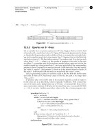
The state diagram corresponding to a transaction appears in Figure 15.1. We say
that a transaction has committed only if it has entered the committed state. Simi-
larly, we say that a transaction has aborted only if it has entered the aborted state. A
transaction is said to have terminated if has either committed or aborted.
A transaction starts in the active state. When it finishes its final statement, it enters
the partially committed state. At this point, the transaction has completed its exe-
cution, but it is still possible that it may have to be aborted, since the actual output
may still be temporarily residing in main memory, and thus a hardware failure may
preclude its successful completion.
The database system then writes out enough information to disk that, even in the
event of a failure, the updates performed by the transaction can be re-created when
the system restarts after the failure. When the last of this information is written out,
the transaction enters the committed state.
As mentioned earlier, we assume for now that failures do not result in loss of data
on disk. Chapter 17 discusses techniques to deal with loss of data on disk.
A transaction enters the failed state after the system determines that the transac-
tion can no longer proceed with its normal execution (for example, because of hard-
ware or logical errors). Such a transaction must be rolled back. Then, it enters the
aborted state. At this point, the system has two options:
Silberschatz−Korth−Sudarshan:

Database System
Concepts, Fourth Edition

V. Transaction
Management
15. Transactions
569
© The McGraw−Hill
Companies, 2001
570 Chapter 15 Transactions
committed
aborted
failed
active
partially
committed
Figure 15.1 State diagram of a transaction.
• It can restart the transaction, but only if the transaction was aborted as a result
of some hardware or software error that was not created through the inter-
nal logic of the transaction. A restarted transaction is considered to be a new
transaction.
• It can kill thetransaction.Itusuallydoessobecauseofsomeinternallogical
error that can be corrected only by rewriting the application program, or be-
causetheinputwasbad,orbecausethedesireddatawerenotfoundinthe
database.
We must be cautious when dealing with observable external writes,suchaswrites
to a terminal or printer. Once such a write has occurred, it cannot be erased, since it
may have been seen external to the database system. Most systems allow such writes
to take place only after the transaction has entered the committed state. One way to
implement such a scheme is for the database system to store any value associated
with such external writes temporarily in nonvolatile storage, and to perform the ac-
tual writes only after the transaction enters the committed state. If the system should
fail after the transaction has entered the committed state, but before it could complete

the external writes, the database system will carry out the external writes (using the
data in nonvolatile storage) when the system is restarted.
Handling external writes can be more complicated in some situations. For example
suppose the external action is that of dispensing cash at an automated teller machine,
and the system fails just before the cash is actually dispensed (we assume that cash
can be dispensed atomically). It makes no sense to dispense cash when the system
is restarted, since the user may have left the machine. In such a case a compensat-
ing transaction, such as depositing the cash back in the users account, needs to be
executed when the system is restarted.
Silberschatz−Korth−Sudarshan:

Database System
Concepts, Fourth Edition
V. Transaction
Management
15. Transactions
570
© The McGraw−Hill
Companies, 2001
15.3 Implementation of Atomicity and Durability 571
For certain applications, it may be desirable to allow active transactions to dis-
play data to users, particularly for long-duration transactions that run for minutes
or hours. Unfortunately, we cannot allow such output of observable data unless we
are willing to compromise transaction atomicity. Most current transaction systems
ensure atomicity and, therefore, forbid this form of interaction with users. In Chapter
24, we discuss alternative transaction models that support long-duration, interactive
transactions.
15.3 Implementation of Atomicity and Durability
The recovery-management component of a database system can support atomicity
and durability by a variety of schemes. We first consider a simple, but extremely in-

efficient, scheme called the shadow copy scheme. This scheme, which is based on
making copies of the database, called shadow copies, assumes that only one transac-
tion is active at a time. The scheme also assumes that the database is simply a file on
disk. A pointer called db-pointer is maintained on disk; it points to the current copy
of the database.
In the shadow-copy scheme, a transaction that wants to update the database first
creates a complete copy of the database. All updates are done on the new database
copy, leaving the original copy, the shadow copy, untouched. If at any point the trans-
action has to be aborted, the system merely deletes the new copy. The old copy of the
database has not been affected.
If the transaction completes, it is committed as follows. First, the operating system
is asked to make sure that all pages of the new copy of the database have been written
out to disk. (Unix systems use the flush command for this purpose.) After the operat-
ing system has written all the pages to disk, the database system updates the pointer
db-pointer to point to the new copy of the database; the new copy then becomes
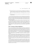
the current copy of the database. The old copy of the database is then deleted. Fig-
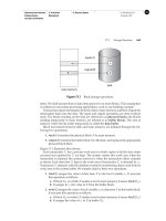
ure 15.2 depicts the scheme, showing the database state before and after the update.
db-pointer
(a) Before update
old copy of
database
(to be deleted)
old copy of
database
db-pointer
(b) After update
new copy of
database
Figure 15.2 Shadow-copy technique for atomicity and durability.
Silberschatz−Korth−Sudarshan:

Database System
Concepts, Fourth Edition
V. Transaction
Management
15. Transactions
571
© The McGraw−Hill
Companies, 2001
572 Chapter 15 Transactions
The transaction is said to have been committed at the point where the updated db-
pointer is written to disk.
We now consider how the technique handles transaction and system failures. First,
consider transaction failure. If the transaction fails at any time before db-pointer is
updated, the old contents of the database are not affected. We can abort the trans-
action by just deleting the new copy of the database. Once the transaction has been
committed, all the updates that it performed are in the database pointed to by db-
pointer. Thus, either all updates of the transaction are reflected, or none of the effects
are reflected, regardless of transaction failure.
Now consider the issue of system failure. Suppose that the system fails at any time
before the updated db-pointer is written to disk. Then, when the system restarts, it
will read db-pointer and will thus see the original contents of the database, and none
of the effects of the transaction will be visible on the database. Next, suppose that the
system fails after db-pointer has been updated on disk. Before the pointer is updated,
all updated pages of the new copy of the database were written to disk. Again, we
assume that, once a file is written to disk, its contents will not be damaged even if
there is a system failure. Therefore, when the system restarts, it will read db-pointer
and will thus see the contents of the database after all the updates performed by the
transaction.
The implementation actually depends on the write to db-pointer being atomic;

that is, either all its bytes are written or none of its bytes are written. If some of the
bytes of the pointer were updated by the write, but others were not, the pointer is
meaningless, and neither old nor new versions of the database may be found when
the system restarts. Luckily, disk systems provide atomic updates to entire blocks, or
at least to a disk sector. In other words, the disk system guarantees that it will update
db-pointer atomically, as long as we make sure that db-pointer lies entirely in a single
sector, which we can ensure by storing db-pointer at the beginning of a block.
Thus, the atomicity and durability properties of transactions are ensured by the
shadow-copy implementation of the recovery-management component.
As a simple example of a transaction outside the database domain, consider a text-
editing session. An entire editing session can be modeled as a transaction. The actions
executed by the transaction are reading and updating the file. Saving the file at the
end of editing corresponds to a commit of the editing transaction; quitting the editing
session without saving the file corresponds to an abort of the editing transaction.
Many text editors use essentially the implementation just described, to ensure that
an editing session is transactional. A new file is used to store the updated file. At the
end of the editing session, if the updated file is to be saved, the text editor uses a file
rename command to rename the new file to have the actual file name. The rename,
assumed to be implemented as an atomic operation by the underlying file system,
deletes the old file as well.
Unfortunately, this implementation is extremely inefficient in the context of large
databases, since executing a single transaction requires copying the entire database.
Furthermore, the implementation does not allow transactions to execute concurrently
with one another. There are practical ways of implementing atomicity and durability
that are much less expensive and more powerful. We study these recovery techniques
in Chapter 17.
Silberschatz−Korth−Sudarshan:

Database System
Concepts, Fourth Edition

V. Transaction
Management
15. Transactions
572
© The McGraw−Hill
Companies, 2001
15.4 Concurrent Executions 573
15.4 Concurrent E xecutions
Transaction-processing systems usually allow multiple transactions to run concur-
rently. Allowing multiple transactions to update data concurrently causes several
complications with consistency of the data, as we saw earlier. Ensuring consistency
in spite of concurrent execution of transactions requires extra work; it is far easier to
insist that transactions run serially—that is, one at a time, each starting only after
the previous one has completed. However, there are two good reasons for allowing
concurrency:
• Improved throughput and resource utilization. A transaction consists of many
steps. Some involve
I/O activity; others involve CPU activity. The CPU and the
disks in a computer system can operate in parallel. Therefore,
I/O activity can
be done in parallel with processing at the
CPU. The parallelism of the CPU
and the I/O system can therefore be exploited to run multiple transactions in
parallel. While a read or write on behalf of one transaction is in progress on
one disk, another transaction can be running in the
CPU, while another disk
may be executing a read or write on behalf of a third transaction. All of this
increases the throughput of the system —that is, the number of transactions
executed in a given amount of time. Correspondingly, the processor and disk
utilization also increase; in other words, the processor and disk spend less

time idle, or not performing any useful work.
• Reduced waiting time. There may be a mix of transactions running on a sys-
tem, some short and some long. If transactions run serially, a short transaction
may have to wait for a preceding long transaction to complete, which can lead
to unpredictable delays in running a transaction. If the transactions are oper-
ating on different parts of the database, it is better to let them run concurrently,
sharing the
CPU cycles and disk accesses among them. Concurrent execution
reduces the unpredictable delays in running transactions. Moreover, it also
reduces the average response time: the average time for a transaction to be
completed after it has been submitted.
The motivation for using concurrent execution in a database is essentially the same
as the motivation for using multiprogramming in an operating system.
When several transactions run concurrently, database consistency can be destroyed
despite the correctness of each individual transaction. In this section, we present the
concept of schedules to help identify those executions that are guaranteed to ensure
consistency.
The database system must control the interaction among the concurrent trans-
actions to prevent them from destroying the consistency of the database. It does
so through a variety of mechanisms called concurrency-control schemes. We study
concurrency-control schemes in Chapter 16; for now, we focus on the concept of cor-
rect concurrent execution.
Consider again the simplified banking system of Section 15.1, which has several
accounts, and a set of transactions that access and update those accounts. Let T
1
and
Silberschatz−Korth−Sudarshan:

Database System
Concepts, Fourth Edition

V. Transaction
Management
15. Transactions
573
© The McGraw−Hill
Companies, 2001
574 Chapter 15 Transactions
T
2
be two transactions that transfer funds from one account to another. Transaction T
1
transfers $50 from account A to account B. It is defined as
T
1
: read(A);
A := A − 50;
write(A);
read(B);
B := B + 50;
write(B).
Transaction T
2
transfers 10 percent of the balance from account A to account B.Itis
defined as
T
2
: read(A);
temp := A *0.1;
A := A − temp;
write(A);

read(B);
B := B + temp;
write(B).
Suppose the current values of accounts A and B are $1000 and $2000, respectively.
Suppose also that the two transactions are executed one at a time in the order T
1
followed by T
2
. This execution sequence appears in Figure 15.3. In the figure, the
sequence of instruction steps is in chronological order from top to bottom, with in-
structions of T
1
appearing in the left column and instructions of T
2
appearing in the
right column. The final values of accounts A and B, after the execution in Figure 15.3
takes place, are $855 and $2145, respectively. Thus, the total amount of money in
T
1
T
2
read(A)
A := A –50
write (A)
read(B)
B := B +50
write(B)
read(A)
temp := A *0.1
A := A – temp

write(A)
read(B)
B := B + temp
write(B)
Figure 15.3 Schedule 1—a serial schedule in which T
1
is followed by T
2
.