Contents Preface v vi ix Acknowledgments A Note to the Student 3.7 3.8 †3.9 3.10 Nodal Versus pdf
Bạn đang xem bản rút gọn của tài liệu. Xem và tải ngay bản đầy đủ của tài liệu tại đây (18.6 MB, 935 trang )
Preface v
Acknowledgments vi
A Note to the Student ix
1.1
Introduction 4
1.2
Systems of Units 4
1.3
Charge and Current 6
1.4
Voltage 9
1.5
Power and Energy 10
1.6
Circuit Elements 13
†
1.7
Applications 15
1.7.1 TV Picture Tube
1.7.2 Electricity Bills
†
1.8
Problem Solving 18
1.9
Summary 21
Review Questions 22
Problems 23
Comprehensive Problems 25
2.1
Introduction 28
2.2
Ohm’s Laws 28
†
2.3
Nodes, Branches, and Loops 33
2.4
Kirchhoff’s Laws 35
2.5
Series Resistors and Voltage Division 41
2.6
Parallel Resistors and Current Division 42
†
2.7
Wye-Delta Transformations 50
†
2.8
Applications 54
2.8.1 Lighting Systems
2.8.2 Design of DC Meters
2.9
Summary 60
Review Questions 61
Problems 63
Comprehensive Problems 72
3.1
Introduction 76
3.2
Nodal Analysis 76
3.3
Nodal Analysis with Voltage Sources 82
3.4
Mesh Analysis 87
3.5
Mesh Analysis with Current Sources 92
†
3.6
Nodal and Mesh Analyses by Inspection 95
3.7
Nodal Versus Mesh Analysis 99
3.8
Circuit Analysis with PSpice 100
†
3.9
Applications: DC Transistor Circuits 102
3.10
Summary 107
Review Questions 107
Problems 109
Comprehensive Problems 117
4.1
Introduction 120
4.2
Linearity Property 120
4.3
Superposition 122
4.4
Source Transformation 127
4.5
Thevenin’s Theorem 131
4.6
Norton’s Theorem 137
†
4.7
Derivations of Thevenin’s and Norton’s
Theorems 140
4.8
Maximum Power Transfer 142
4.9
Verifying Circuit Theorems
with PSpice 144
†
4.10
Applications 147
4.10.1 Source Modeling
4.10.2 Resistance Measurement
4.11
Summary 153
Review Questions 153
Problems 154
Comprehensive Problems 162
5.1
Introduction 166
5.2
Operational Amplifiers 166
5.3
Ideal Op Amp 170
5.4
Inverting Amplifier 171
5.5
Noninverting Amplifier 174
5.6
Summing Amplifier 176
5.7
Difference Amplifier 177
5.8
Cascaded Op Amp Circuits 181
5.9
Op Amp Circuit Analysis
with PSpice 183
†
5.10
Applications 185
5.10.1 Digital-to Analog Converter
5.10.2 Instrumentation Amplifiers
5.11
Summary 188
Review Questions 190
Problems 191
Comprehensive Problems 200
Contents
xi
Chapter 2 Basic Laws 27
Chapter 3 Methods of Analysis 75
PART 1 DC CIRCUITS 1
Chapter 1 Basic Concepts 3
Chapter 4 Circuit Theorems 119
Chapter 5 Operational Amplifiers 165
f51-cont.qxd 3/16/00 4:22 PM Page xi
6.1
Introduction 202
6.2
Capacitors 202
6.3
Series and Parallel Capacitors 208
6.4
Inductors 211
6.5
Series and Parallel Inductors 216
†
6.6
Applications 219
6.6.1 Integrator
6.6.2 Differentiator
6.6.3 Analog Computer
6.7
Summary 225
Review Questions 226
Problems 227
Comprehensive Problems 235
7.1
Introduction 238
7.2
The Source-free RC Circuit 238
7.3
The Source-free RL Circuit 243
7.4
Singularity Functions 249
7.5
Step Response of an RC Circuit 257
7.6
Step Response of an RL Circuit 263
†
7.7
First-order Op Amp Circuits 268
7.8
Transient Analysis with PSpice 273
†
7.9
Applications 276
7.9.1 Delay Circuits
7.9.2 Photoflash Unit
7.9.3 Relay Circuits
7.9.4 Automobile Ignition Circuit
7.10
Summary 282
Review Questions 283
Problems 284
Comprehensive Problems 293
8.1
Introduction 296
8.2
Finding Initial and Final Values 296
8.3
The Source-Free Series RLC Circuit 301
8.4
The Source-Free Parallel RLC Circuit 308
8.5
Step Response of a Series RLC
Circuit 314
8.6
Step Response of a Parallel RLC
Circuit 319
8.7
General Second-Order Circuits 322
8.8
Second-Order Op Amp Circuits 327
8.9
PSpice Analysis of RLC Circuits 330
†
8.10
Duality 332
†
8.11
Applications 336
8.11.1 Automobile Ignition System
8.11.2 Smoothing Circuits
8.12
Summary 340
Review Questions 340
Problems 341
Comprehensive Problems 350
9.1
Introduction 354
9.2
Sinusoids 355
9.3
Phasors 359
9.4
Phasor Relationships for Circuit
Elements 367
9.5
Impedance and Admittance 369
9.6
Kirchhoff’s Laws in the Frequency
Domain 372
9.7
Impedance Combinations 373
†
9.8
Applications 379
9.8.1 Phase-Shifters
9.8.2 AC Bridges
9.9
Summary 384
Review Questions 385
Problems 385
Comprehensive Problems 392
10.1
Introduction 394
10.2
Nodal Analysis 394
10.3
Mesh Analysis 397
10.4
Superposition Theorem 400
10.5
Source Transformation 404
10.6
Thevenin and Norton Equivalent
Circuits 406
10.7
Op Amp AC Circuits 411
10.8
AC Analysis Using PSpice 413
†
10.9
Applications 416
10.9.1 Capacitance Multiplier
10.9.2 Oscillators
10.10
Summary 420
Review Questions 421
Problems 422
11.1
Introduction 434
11.2
Instantaneous and Average Power 434
11.3
Maximum Average Power Transfer 440
11.4
Effective or RMS Value 443
11.5
Apparent Power and Power Factor 447
11.6
Complex Power 449
†
11.7
Conservation of AC Power 453
xii
CONTENTS
Chapter 8 Second-Order Circuits 295
Chapter 10 Sinusoidal Steady-State Analysis 393
Chapter 11 AC Power Analysis 433
Chapter 6 Capacitors and Inductors 201
Chapter 7 First-Order Circuits 237
PART 2 AC CIRCUITS 351
Chapter 9 Sinusoids and Phasors 353
11.8
Power Factor Correction 457
†
11.9
Applications 459
11.9.1 Power Measurement
11.9.2 Electricity Consumption Cost
11.10
Summary 464
Review Questions 465
Problems 466
Comprehensive Problems 474
12.1
Introduction 478
12.2
Balanced Three-Phase Voltages 479
12.3
Balanced Wye-Wye Connection 482
12.4
Balanced Wye-Delta Connection 486
12.5
Balanced Delta-Delta Connection 488
12.6
Balanced Delta-Wye Connection 490
12.7
Power in a Balanced System 494
†
12.8
Unbalanced Three-Phase Systems 500
12.9
PSpice for Three-Phase Circuits 504
†
12.10
Applications 508
12.10.1 Three-Phase Power Measurement
12.10.2 Residential Wiring
12.11
Summary 516
Review Questions 517
Problems 518
Comprehensive Problems 525
13.1
Introduction 528
13.2
Mutual Inductance 528
13.3
Energy in a Coupled Circuit 535
13.4
Linear Transformers 539
13.5
Ideal Transformers 545
13.6
Ideal Autotransformers 552
†
13.7
Three-Phase Transformers 556
13.8
PSpice Analysis of Magnetically Coupled
Circuits 559
†
13.9
Applications 563
13.9.1 Transformer as an Isolation Device
13.9.2 Transformer as a Matching Device
13.9.3 Power Distribution
13.10
Summary 569
Review Questions 570
Problems 571
Comprehensive Problems 582
14.1
Introduction 584
14.2
Transfer Function 584
†
14.3
The Decibel Scale 588
14.4
Bode Plots 589
14.5
Series Resonance 600
14.6
Parallel Resonance 605
14.7
Passive Filters 608
14.7.1 Lowpass Filter
14.7.2 Highpass Filter
14.7.3 Bandpass Filter
14.7.4 Bandstop Filter
14.8
Active Filters 613
14.8.1 First-Order Lowpass Filter
14.8.2 First-Order Highpass Filter
14.8.3 Bandpass Filter
14.8.4 Bandreject (or Notch) Filter
†
14.9
Scaling 619
14.9.1 Magnitude Scaling
14.9.2 Frequency Scaling
14.9.3 Magnitude and Frequency Scaling
14.10
Frequency Response Using
PSpice 622
†
14.11
Applications 626
14.11.1 Radio Receiver
14.11.2 Touch-Tone Telephone
14.11.3 Crossover Network
14.12
Summary 631
Review Questions 633
Problems 633
Comprehensive Problems 640
15.1
Introduction 646
15.2
Definition of the Laplace
Transform 646
15.3
Properties of the Laplace
Transform 649
15.4
The Inverse Laplace Transform 659
15.4.1 Simple Poles
15.4.2 Repeated Poles
15.4.3 Complex Poles
15.5
Applicaton to Circuits 666
15.6
Transfer Functions 672
15.7
The Convolution Integral 677
†
15.8
Application to Integrodifferential
Equations 685
†
15.9
Applications 687
15.9.1 Network Stability
15.9.2 Network Synthesis
15.10
Summary 694
xiii
CONTENTS
PART 3 ADVANCED CIRCUIT ANALYSIS 643
Chapter 15 The Laplace Transform 645
Chapter 12 Three-Phase Circuits 477
Chapter 13 Magnetically Coupled Circuits 527
Chapter 14 Frequency Response 583
Review Questions 696
Problems 696
Comprehensive Problems 705
16.1
Introduction 708
16.2
Trigonometric Fourier Series 708
16.3
Symmetry Considerations 717
16.3.1 Even Symmetry
16.3.2 Odd Symmetry
16.3.3 Half-Wave Symmetry
16.4
Circuit Applicatons 727
16.5
Average Power and RMS Values 730
16.6
Exponential Fourier Series 734
16.7
Fourier Analysis with PSpice 740
16.7.1 Discrete Fourier Transform
16.7.2 Fast Fourier Transform
†
16.8
Applications 746
16.8.1 Spectrum Analyzers
16.8.2 Filters
16.9
Summary 749
Review Questions 751
Problems 751
Comprehensive Problems 758
17.1
Introduction 760
17.2
Definition of the Fourier Transform 760
17.3
Properties of the Fourier Transform 766
17.4
Circuit Applications 779
17.5
Parseval’s Theorem 782
17.6
Comparing the Fourier and Laplace
Transforms 784
†
17.7
Applications 785
17.7.1 Amplitude Modulation
17.7.2 Sampling
17.8
Summary 789
Review Questions 790
Problems 790
Comprehensive Problems 794
18.1
Introduction 796
18.2
Impedance Parameters 796
18.3
Admittance Parameters 801
18.4
Hybrid Parameters 804
18.5
Transmission Parameters 809
†
18.6
Relationships between Parameters 814
18.7
Interconnection of Networks 817
18.8
Computing Two-Port Parameters Using
PSpice 823
†
18.9
Applications 826
18.9.1 Transistor Circuits
18.9.2 Ladder Network Synthesis
18.10
Summary 833
Review Questions 834
Problems 835
Comprehensive Problems 844
Appendix A
Solution of Simultaneous Equations Using
Cramer’s Rule 845
Appendix B
Complex Numbers 851
Appendix C
Mathematical Formulas 859
Appendix D
PSpice for Windows 865
Appendix E
Answers to Odd-Numbered Problems 893
Selected Bibliography
929
Index
933
xiv
CONTENTS
Chapter 16 The Fourier Series 707
Chapter 17 Fourier Transform 759
Chapter 18 Two-Port Networks 795
Features
In spite of the numerous textbooks on circuit analysis
available in the market, students often find the course
difficult to learn. The main objective of this book is
to present circuit analysis in a manner that is clearer,
more interesting, and easier to understand than earlier
texts. This objective is achieved in the following
ways:
• A course in circuit analysis is perhaps the first
exposure students have to electrical engineering.
We have included several features to help stu-
dents feel at home with the subject. Each chapter
opens with either a historical profile of some
electrical engineering pioneers to be mentioned in
the chapter or a career discussion on a subdisci-
pline of electrical engineering. An introduction
links the chapter with the previous chapters and
states the chapter’s objectives. The chapter ends
with a summary of the key points and formulas.
• All principles are presented in a lucid, logical,
step-by-step manner. We try to avoid wordiness
and superfluous detail that could hide concepts
and impede understanding the material.
• Important formulas are boxed as a means of
helping students sort what is essential from what
is not; and to ensure that students clearly get the
gist of the matter, key terms are defined and
highlighted.
• Marginal notes are used as a pedagogical aid. They
serve multiple uses—hints, cross-references, more
exposition, warnings, reminders, common mis-
takes, and problem-solving insights.
• Thoroughly worked examples are liberally given at
the end of every section. The examples are regard-
ed as part of the text and are explained clearly, with-
out asking the reader to fill in missing steps.
Thoroughly worked examples give students a good
understanding of the solution and the confidence to
solve problems themselves. Some of the problems
are solved in two or three ways to facilitate an
understanding and comparison of different
approaches.
• To give students practice opportunity, each illus-
trative example is immediately followed by a
practice problem with the answer. The students can
follow the example step-by-step to solve the prac-
tice problem without flipping pages or searching
the end of the book for answers. The practice prob-
lem is also intended to test students’ understanding
of the preceding example. It will reinforce their
grasp of the material before moving to the next
section.
• In recognition of ABET’s requirement on integrat-
ing computer tools, the use of PSpice is encouraged
in a student-friendly manner. Since the Windows
version of PSpice is becoming popular, it is used
instead of the MS-DOS version. PSpice is covered
early so that students can use it throughout the text.
Appendix D serves as a tutorial on PSpice for
Windows.
• The operational amplifier (op amp) as a basic ele-
ment is introduced early in the text.
• To ease the transition between the circuit course
and signals/systems courses, Fourier and Laplace
transforms are covered lucidly and thoroughly.
• The last section in each chapter is devoted to appli-
cations of the concepts covered in the chapter. Each
chapter has at least one or two practical problems or
devices. This helps students apply the concepts to
real-life situations.
• Ten multiple-choice review questions are provided
at the end of each chapter, with answers. These are
intended to cover the little “tricks” that the exam-
ples and end-of-chapter problems may not cover.
They serve as a self-test device and help students
determine how well they have mastered the chapter.
Organization
This book was written for a two-semester or three-semes-
ter course in linear circuit analysis. The book may
also be used for a one-semester course by a proper selec-
tion of chapters and sections. It is broadly divided into
three parts.
• Part 1, consisting of Chapters 1 to 8, is devoted to
dc circuits. It covers the fundamental laws and the-
orems, circuit techniques, passive and active ele-
ments.
• Part 2, consisting of Chapters 9 to 14, deals with ac
circuits. It introduces phasors, sinusoidal steady-
state analysis, ac power, rms values, three-phase
systems, and frequency response.
• Part 3, consisting of Chapters 15 to 18, is devoted
to advanced techniques for network analysis.
It provides a solid introduction to the Laplace
transform, Fourier series, the Fourier transform,
and two-port network analysis.
The material in three parts is more than suffi-
cient for a two-semester course, so that the instructor
PREFACE
v
F51-pref.qxd 3/17/00 10:11 AM Page v
must select which chapters/sections to cover. Sections
marked with the dagger sign (†) may be skipped,
explained briefly, or assigned as homework. They can
be omitted without loss of continuity. Each chapter has
plenty of problems, grouped according to the sections
of the related material, and so diverse that the instruc-
tor can choose some as examples and assign some as
homework. More difficult problems are marked with a
star (*). Comprehensive problems appear last; they are
mostly applications problems that require multiple
skills from that particular chapter.
The book is as self-contained as possible. At the
end of the book are some appendixes that review
solutions of linear equations, complex numbers, math-
ematical formulas, a tutorial on PSpice for Windows,
and answers to odd-numbered problems. Answers to
all the problems are in the solutions manual, which is
available from the publisher.
Prerequisites
As with most introductory circuit courses, the main
prerequisites are physics and calculus. Although famil-
iarity with complex numbers is helpful in the later part
of the book, it is not required.
Supplements
Solutions Manual—an Instructor’s Solutions Manual is
available to instructors who adopt the text. It contains
complete solutions to all the end-of-chapter problems.
Transparency Masters—over 200 important figures
are available as transparency masters for use as over-
heads.
Student CD-ROM—100 circuit files from the book are
presented as Electronics Workbench (EWB) files; 15–20
of these files are accessible using the free demo of Elec-
tronics Workbench. The students are able to experiment
with the files. For those who wish to fully unlock all 100
circuit files, EWB’s full version may be purchased from
Interactive Image Technologies for approximately
$79.00. The CD-ROM also contains a selection of prob-
lem-solving, analysis and design tutorials, designed to
further support important concepts in the text.
Problem-Solving Workbook—a paperback work-
book is for sale to students who wish to practice their
problem solving techniques. The workbook contains a
discussion of problem solving strategies and 150 addi-
tional problems with complete solutions provided.
Online Learning Center (OLC)—the Web site for
the book will serve as an online learning center for stu-
dents as a useful resource for instructors. The OLC
will provide access to:
300 test questions—for instructors only
Downloadable figures for overhead
presentations—for instructors only
Solutions manual—for instructors only
Web links to useful sites
Sample pages from the Problem-Solving
Workbook
PageOut Lite—a service provided to adopters
who want to create their own Web site. In
just a few minutes, instructors can change
the course syllabus into a Web site using
PageOut Lite.
The URL for the web site is www.mhhe.com.alexander.
Although the textbook is meant to be self-explanatory
and act as a tutor for the student, the personal contact
involved in teaching is not to be forgotten. The book
and supplements are intended to supply the instructor
with all the pedagogical tools necessary to effectively
present the material.
We wish to take the opportunity to thank the staff of
McGraw-Hill for their commitment and hard
work: Lynn Cox, Senior Editor; Scott Isenberg,
Senior Sponsoring Editor; Kelley Butcher, Senior
Developmental Editor; Betsy Jones, Executive
Editor; Catherine Fields, Sponsoring Editor;
Kimberly Hooker, Project Manager; and Michelle
Flomenhoft, Editorial Assistant. They got numerous
reviews, kept the book on track, and helped in many
ways. We really appreciate their inputs. We are
greatly in debt to Richard Mickey for taking the pain
ofchecking and correcting the entire manuscript. We
wish to record our thanks to Steven Durbin at Florida
State University and Daniel Moore at Rose Hulman
Institute of Technology for serving as accuracy
checkers of examples, practice problems, and end-
of-chapter problems. We also wish to thank the fol-
lowing reviewers for their constructive criticisms
and helpful comments.
Promod Vohra, Northern Illinois University
Moe Wasserman, Boston University
Robert J. Krueger, University of Wisconsin
Milwaukee
John O’Malley, University of Florida
vi
PREFACE
ACKNOWLEDGMENTS
F51-pref.qxd 3/17/00 10:11 AM Page vi
Aniruddha Datta, Texas A&M University
John Bay, Virginia Tech
Wilhelm Eggimann, Worcester Polytechnic
Institute
A. B. Bonds, Vanderbilt University
Tommy Williamson, University of Dayton
Cynthia Finelli, Kettering University
John A. Fleming, Texas A&M University
Roger Conant, University of Illinois
at Chicago
Daniel J. Moore, Rose-Hulman Institute of
Technology
Ralph A. Kinney, Louisiana State University
Cecilia Townsend, North Carolina State
University
Charles B. Smith, University of Mississippi
H. Roland Zapp, Michigan State University
Stephen M. Phillips, Case Western University
Robin N. Strickland, University of Arizona
David N. Cowling, Louisiana Tech University
Jean-Pierre R. Bayard, California State
University
Jack C. Lee, University of Texas at Austin
E. L. Gerber, Drexel University
The first author wishes to express his apprecia-
tion to his department chair, Dr. Dennis Irwin, for his
outstanding support. In addition, he is extremely grate-
ful to Suzanne Vazzano for her help with the solutions
manual.
The second author is indebted to Dr. Cynthia
Hirtzel, the former dean of the college of engineering
at Temple University, and Drs Brian Butz, Richard
Klafter, and John Helferty, his departmental chairper-
sons at different periods, for their encouragement while
working on the manuscript. The secretarial support
provided by Michelle Ayers and Carol Dahlberg is
gratefully appreciated. Special thanks are due to Ann
Sadiku, Mario Valenti, Raymond Garcia, Leke and
Tolu Efuwape, and Ope Ola for helping in various
ways. Finally, we owe the greatest debt to our wives,
Paulette and Chris, without whose constant support and
cooperation this project would have been impossible.
Please address comments and corrections to the
publisher.
C. K. Alexander and M. N. O. Sadiku
PREFACE
vii
F51-pref.qxd 3/17/00 10:11 AM Page vii
F51-pref.qxd 3/17/00 10:11 AM Page viii
This may be your first course in electrical engineer-
ing. Although electrical engineering is an exciting and
challenging discipline, the course may intimidate you.
This book was written to prevent that. A good textbook
and a good professor are an advantage—but you are
the one who does the learning. If you keep the follow-
ing ideas in mind, you will do very well in this course.
• This course is the foundation on which most
other courses in the electrical engineering cur-
riculum rest. For this reason, put in as much
effort as you can. Study the course regularly.
• Problem solving is an essential part of the learn-
ing process. Solve as many problems as you can.
Begin by solving the practice problem following
each example, and then proceed to the end-of-
chapter problems. The best way to learn is to
solve a lot of problems. An asterisk in front of a
problem indicates a challenging problem.
• Spice, a computer circuit analysis program, is
used throughout the textbook. PSpice, the per-
sonal computer version of Spice, is the popular
standard circuit analysis program at most uni-
versities. PSpice for Windows is described in
Appendix D. Make an effort to learn PSpice,
because you can check any circuit problem with
PSpice and be sure you are handing in a correct
problem solution.
• Each chapter ends with a section on how the
material covered in the chapter can be applied to
real-life situations. The concepts in this section
may be new and advanced to you. No doubt, you
will learn more of the details in other courses.
We are mainly interested in gaining a general
familiarity with these ideas.
• Attempt the review questions at the end of each
chapter. They will help you discover some
“tricks” not revealed in class or in the textbook.
A short review on finding determinants is cov-
ered in Appendix A, complex numbers in Appendix B,
and mathematical formulas in Appendix C. Answers to
odd-numbered problems are given in Appendix E.
Have fun!
C.K.A. and M.N.O.S.
A NOTE TO THE STUDENT
ix
F51-pref.qxd 3/17/00 10:11 AM Page ix
1
DC CIRCUITS
PART 1
Chapter
1
Basic Concepts
Chapter
2
Basic Laws
Chapter
3
Methods of Analysis
Chapter
4
Circuit Theorems
Chapter
5
Operational Amplifier
Chapter
6
Capacitors and Inductors
Chapter
7
First-Order Circuits
Chapter
8
Second-Order Circuits
2
3
CHAPTER
BASICCONCEPTS
1
It is engineering that changes the world.
—Isaac Asimov
Historical Profiles
Alessandro Antonio Volta (1745–1827), an Italian physicist, invented the electric
battery—which provided the first continuous flow of electricity—and the capacitor.
Born into a noble family in Como, Italy, Volta was performing electrical
experiments at age 18. His invention of the battery in 1796 revolutionized the use of
electricity. The publication of his work in 1800 marked the beginning of electric circuit
theory. Volta received many honors during his lifetime. The unit of voltage or potential
difference, the volt, was named in his honor.
Andre-Marie Ampere (1775–1836), a French mathematician and physicist, laid the
foundation of electrodynamics. He defined the electric current and developed a way to
measure it in the 1820s.
Born in Lyons, France, Ampere at age 12 mastered Latin in a few weeks, as he
was intensely interested in mathematics and many of the best mathematical works were
in Latin. He was a brilliant scientist and a prolific writer. He formulated the laws of
electromagnetics. He invented the electromagnet and the ammeter. The unit of electric
current, the ampere, was named after him.
4 PART 1 DC Circuits
1.1 INTRODUCTION
Electric circuit theory and electromagnetic theory are the two fundamen-
tal theories upon which all branches of electrical engineering are built.
Many branches of electrical engineering, such as power, electric ma-
chines, control, electronics, communications, and instrumentation, are
based on electric circuit theory. Therefore, the basic electric circuit the-
ory course is the most important course for an electrical engineering
student, and always an excellent starting point for a beginning student
in electrical engineering education. Circuit theory is also valuable to
students specializing in other branches of the physical sciences because
circuits are a good model for the study of energy systems in general, and
because of the applied mathematics, physics, and topology involved.
In electrical engineering, we are often interested in communicating
or transferring energy from one point to another. To do this requires an
interconnection of electrical devices. Such interconnection is referred to
as an electric circuit, and each component of the circuit is known as an
element.
An electric circuit is an interconnection of electrical elements.
A simple electric circuit is shown in Fig. 1.1. It consists of three
basic components: a battery, alamp,and connecting wires. Such a simple
circuit can exist by itself; it has several applications, such as a torch light,
a search light, and so forth.
+
−
Current
Lamp
Battery
Figure 1.1
A simple electric circuit.
A complicated real circuit is displayed in Fig. 1.2, representing the
schematic diagram for a radio receiver. Although it seems complicated,
this circuit can be analyzed using the techniques we cover in this book.
Our goalin thistext is to learnvariousanalytical techniquesand computer
software applications for describing the behavior of a circuit like this.
Electric circuits are used in numerous electrical systems to accom-
plish different tasks. Our objective in this book is not the study of various
uses and applications of circuits. Rather our major concern is the anal-
ysis of the circuits. By the analysis of a circuit, we mean a study of the
behavior of the circuit: How does it respond to a given input? How do
the interconnected elements and devices in the circuit interact?
We commence our study by defining some basic concepts. These
concepts include charge, current, voltage, circuit elements, power, and
energy. Before defining these concepts, we must first establish a system
of units that we will use throughout the text.
1.2SYSTEMSOFUNITS
As electrical engineers, we deal with measurable quantities. Our mea-
surement, however, must be communicated in a standard language that
virtually all professionals can understand, irrespective of the country
where the measurement is conducted. Such an international measure-
ment language is the International System of Units (SI), adopted by the
General Conference on Weights and Measures in 1960. In this system,
CHAPTER 1 Basic Concepts 5
2, 5, 6
C
Oscillator
E
B
R2
10 k
R3
10 k
R1 47
Y1
7 MHz
C6 5
L2
22.7 mH
(see text)
to
U1, Pin 8
R10
10 k
GAIN
+
+
C16
100 mF
16 V
C11
100 mF
16 V
C10
1.0 mF
16 V
C9
1.0 mF
16 V
C15
0.47
16 V
C17
100 mF
16 V
+
−
12-V dc
Supply
Audio
Output
+
C18
0.1
R12
10
1
4
2
3
C14
0.0022
0.1C13
U2A
1⁄2 TL072
U2B
1⁄2 TL072
R9
15 k
R5
100 k
R8
15 k
R6
100 k
5
6
R7
1 M
C12
0.0033
+
L3
1 mH
R11
47
C8
0.1
Q1
2N2222A
7
C3 0.1
L1
0.445 mH
Antenna
C1
2200 pF
C2
2200 pF
1
8
7
U1
SBL-1
Mixer
3, 4
C7
532
C4
910
C5
910
R4
220
U3
LM386N
Audio power amp
5
4
6
3
2
+
+
−
+
−
+
−
+
8
Figure 1.2
Electric circuit of a radio receiver.
(Reproduced with permission from QST, August 1995, p. 23.)
there are six principal units from which the units of all other physical
quantities can be derived. Table 1.1 shows the six units, their symbols,
and the physical quantities they represent. The SI units are used through-
out this text.
One great advantage of the SI unit is that it uses prefixes based on
the power of 10 to relate larger and smaller units to the basic unit. Table
1.2 shows the SI prefixes and their symbols. For example, the following
are expressions of the same distance in meters (m):
600,000,000 mm 600,000 m 600 km
TABLE 1.2
The SI prefixes.
Multiplier Prefix Symbol
10
18
exa E
10
15
peta P
10
12
tera T
10
9
giga G
10
6
mega M
10
3
kilo k
10
2
hecto h
10 deka da
10
−1
deci d
10
−2
centi c
10
−3
milli m
10
−6
micro µ
10
−9
nano n
10
−12
pico p
10
−15
femto f
10
−18
atto a
TABLE 1.1
The six basic SI units.
Quantity Basic unit Symbol
Length meter m
Mass kilogram kg
Time second s
Electric current ampere A
Thermodynamic temperature kelvin K
Luminous intensity candela cd
6 PART 1 DC Circuits
1.3CHARGEANDCURRENT
The concept of electric charge is the underlying principle for explaining
all electrical phenomena. Also, the most basic quantity in an electric
circuit is the electric charge. We all experience the effect of electric
charge when we try to remove our wool sweater and have it stick to our
body or walk across a carpet and receive a shock.
Charge is an electrical property of the atomic particles of which
matter consists, measured in coulombs (C).
We know from elementary physics that all matter is made of fundamental
building blocks known as atoms and that each atom consists of electrons,
protons, and neutrons. We also know that the charge e on an electron is
negativeand equal inmagnitude to1.602×10
−19
C, while aproton carries
a positive charge of the same magnitude as the electron. The presence of
equal numbers of protons and electrons leaves an atom neutrally charged.
The following points should be noted about electric charge:
1. The coulomb is a large unit for charges. In1Cofcharge, there
are 1/(1.602 × 10
−19
) = 6.24 × 10
18
electrons. Thus realistic
or laboratory values of charges are on the order of pC, nC, or
µC.
1
2. According to experimental observations, the only charges that
occur in nature are integral multiples of the electronic charge
e =−1.602 × 10
−19
C.
3. The law of conservation of charge states that charge can neither
be created nor destroyed, only transferred. Thus the algebraic
sum of the electric charges in a system does not change.
We now consider the flow of electric charges. A unique feature of
electric charge or electricity is the fact that it is mobile; that is, it can
be transferred from one place to another, where it can be converted to
another form of energy.
Battery
I
−−
−−
+
−
Figure 1.3
Electric current due to flow
of electronic charge in a conductor.
A convention is a standard way of describing
something so that others in the profession can
understand what we mean. We will be using IEEE
conventions throughout this book.
When a conducting wire (consisting of several atoms) is connected
to a battery (a source of electromotive force), the charges are compelled
to move; positive charges move in one direction while negative charges
move in the opposite direction. This motion of charges creates electric
current. It is conventional to take the current flow as the movement of
positive charges, that is, opposite to the flow of negative charges, as Fig.
1.3 illustrates. This convention was introduced by Benjamin Franklin
(1706–1790), the American scientist and inventor. Although we now
know that current in metallic conductors is due to negatively charged
electrons, we will follow the universally accepted convention that current
is the net flow of positive charges. Thus,
1
However, a large power supply capacitor can store up to 0.5 C of charge.
CHAPTER 1 Basic Concepts 7
Electric current is the time rate of change of charge, measured in amperes (A).
Mathematically, the relationship between current i, charge q, and time t
is
i =
dq
dt
(1.1)
where current is measured in amperes (A), and
1 ampere = 1 coulomb/second
The charge transferred between time t
0
and t is obtained by integrating
both sides of Eq. (1.1). We obtain
q =
t
t
0
idt
(1.2)
Thewaywedefine current as i in Eq. (1.1) suggests that current need not
be a constant-valued function. As many of the examples and problems in
this chapter and subsequent chapters suggest, there can be several types
of current; that is, charge can vary with time in several ways that may be
represented by different kinds of mathematical functions.
If the current does not change with time, but remains constant, we
call it a direct current (dc).
A direct current (dc) is a current that remains constant with time.
By convention the symbol I is used to represent such a constant current.
A time-varying current is represented by the symbol i. A com-
mon form of time-varying current is the sinusoidal current or alternating
current (ac).
An alternating current (ac) is a current that varies sinusoidally with time.
Such current is used in your household, to run the air conditioner, refrig-
erator, washing machine, and other electric appliances. Figure 1.4 shows
direct current and alternating current; these are the two most common
types of current. We will consider other types later in the book.
I
0
t
(a)
(b)
i
t
0
Figure 1.4
Two common types of
current: (a) direct current (dc),
(b) alternating current (ac).
Once we define current as the movement of charge, we expect cur-
rent to have an associated direction of flow. As mentioned earlier, the
directionofcurrentflowisconventionallytakenasthedirectionofpositive
charge movement. Based on this convention, a current of 5 A may be
represented positively or negatively as shown in Fig. 1.5. In other words,
a negative current of −5Aflowing in one direction as shown in Fig.
1.5(b) is the same as a current of +5Aflowing in the opposite direction.
5 A
(a)
−5 A
(b)
Figure 1.5
Conventional current flow:
(a) positive current flow, (b) negative current
flow.
8 PART 1 DC Circuits
EXAMPLE 1.1
How much charge is represented by 4,600 electrons?
Solution:
Each electron has −1.602 × 10
−19
C. Hence 4,600 electrons will have
−1.602 × 10
−19
C/electron × 4,600 electrons =−7.369 ×10
−16
C
PRACTICE PROBLEM 1.1
Calculate the amount of charge represented by two million protons.
Answer: +3.204 × 10
−13
C.
EXAMPLE 1.2
The total charge entering a terminal is given by q = 5t sin 4πt mC. Cal-
culate the current at t = 0.5s.
Solution:
i =
dq
dt
=
d
dt
(5t sin 4πt) mC/s = (5 sin4πt + 20πt cos 4πt) mA
At t = 0.5,
i = 5 sin2π + 10π cos 2π = 0 +10π = 31.42 mA
PRACTICE PROBLEM 1.2
If in Example 1.2, q = (10 − 10e
−2t
) mC, find the current at t = 0.5s.
Answer: 7.36 mA.
EXAMPLE 1.3
Determinethe totalchargeenteringa terminalbetweent = 1sand t = 2s
if the current passing the terminal is i = (3t
2
− t) A.
Solution:
q =
2
t=1
idt =
2
1
(3t
2
− t) dt
=
t
3
−
t
2
2
2
1
= (8 − 2) −
1 −
1
2
= 5.5C
PRACTICE PROBLEM 1.3
The current flowing through an element is
i =
2A, 0 <t<1
2t
2
A,t>1
Calculate the charge entering the element from t = 0tot = 2s.
Answer: 6.667 C.
CHAPTER 1 Basic Concepts 9
1.4VOLTAGE
As explained briefly in the previous section, to move the electron in a
conductor in a particular direction requires some work or energy transfer.
Thisworkisperformedby anexternalelectromotiveforce(emf), typically
represented by the battery in Fig. 1.3. This emf is also known as voltage
or potential difference. The voltage v
ab
between two points a and b in
an electric circuit is the energy (or work) needed to move a unit charge
from a to b; mathematically,
v
ab
=
dw
dq
(1.3)
where w is energy in joules (J) and q is charge in coulombs (C). The
voltage v
ab
or simply v is measured in volts (V), named in honor of the
Italian physicist Alessandro Antonio Volta (1745–1827), who invented
the first voltaic battery. From Eq. (1.3), it is evident that
1 volt = 1 joule/coulomb = 1 newton meter/coulomb
Thus,
Voltage (or potential difference) is the energy required to move
a unit charge through an element, measured in volts (V).
Figure 1.6 shows the voltage across an element (represented by a
rectangular block) connected to points a and b . The plus (+) and minus
(−) signs are used to define reference direction or voltage polarity. The
v
ab
can be interpreted in two ways: (1) point a is at a potential of v
ab
volts higher than point b, or (2) the potential at point a with respect to
point b is v
ab
. It follows logically that in general
v
ab
=−v
ba
(1.4)
For example, in Fig. 1.7, we have two representations of the same vol-
tage. In Fig.1.7(a), point a is +9V abovepoint b; in Fig. 1.7(b), pointb is
−9 V above pointa. We may say that in Fig. 1.7(a), there is a 9-V voltage
drop from a to b or equivalently a 9-V voltage rise from b to a. In other
words, a voltage drop from a to b is equivalent to a voltage rise from
b to a.
a
b
v
ab
+
−
Figure 1.6
Polarity
of voltage v
ab
.
9 V
(a)
a
b
+
−
−9 V
(b)
a
b
+
−
Figure 1.7
Two equivalent
representations of the same
voltage v
ab
: (a) point a is9V
above point b, (b) point b is
−9 V above point a.
Current and voltage are the two basic variables in electric circuits.
The common term signal is used for an electric quantity such as a current
or a voltage (or even electromagnetic wave) when it is used for conveying
information. Engineers prefer to call such variables signals rather than
mathematical functions of time because of their importance in commu-
nications and other disciplines. Like electric current, a constant voltage
is called a dc voltage and is represented by V, whereas a sinusoidally
time-varying voltage is called an ac voltage and is represented by v.A
dc voltage is commonly produced by a battery; ac voltage is produced by
an electric generator.
Keep in mind that electric current is always
through an element and that electric voltage is al-
ways across the element or between two points.
10 PART 1 DC Circuits
1.5POWERANDENERGY
Although current and voltage are the two basic variables in an electric
circuit, they are not sufficient by themselves. For practical purposes,
we need to know how much power an electric device can handle. We
all know from experience that a 100-watt bulb gives more light than a
60-watt bulb. We also know that when we pay our bills to the electric
utility companies, we are paying for the electric energy consumed over a
certain period of time. Thus power and energy calculations are important
in circuit analysis.
To relate power and energy to voltage and current, we recall from
physics that:
Power is the time rate of expending or absorbing energy, measured in watts (W).
We write this relationship as
p =
dw
dt
(1.5)
where p is power in watts (W), w is energy in joules (J), and t is time in
seconds (s). From Eqs. (1.1), (1.3), and (1.5), it follows that
p =
dw
dt
=
dw
dq
·
dq
dt
= vi
(1.6)
or
p = vi
(1.7)
The power p in Eq. (1.7) is a time-varying quantity and is called the
instantaneouspower. Thus,thepowerabsorbedorsuppliedbyanelement
is the product of the voltage across the element and the current through
it. If the power has a + sign, power is being delivered to or absorbed
by the element. If, on the other hand, the power has a − sign, power is
being supplied by the element. But how do we know when the power has
a negative or a positive sign?
Current direction and voltage polarity play a major role in deter-
mining the sign of power. It is therefore important that we pay attention
to the relationshipbetween current i and voltage v in Fig.1.8(a). The vol-
tage polarity andcurrent direction must conform with those shown inFig.
1.8(a) in order for the power to have a positive sign. This is known as
the passive sign convention. By the passive sign convention, current en-
ters through the positive polarity of the voltage. In this case, p =+vi or
vi > 0 impliesthat theelement isabsorbing power. However, ifp =−vi
or vi < 0, as in Fig. 1.8(b), the element is releasing or supplying power.
p = +vi
(a)
v
+
−
p = −vi
(b)
v
+
−
i
i
Figure 1.8
Reference
polarities for power using
the passive sign conven-
tion: (a) absorbing power,
(b) supplying power.
Passive sign convention is satisfied when the current enters through
the positive terminal of an element and p =+vi. If the current
enters through the negative terminal, p =−vi.
CHAPTER 1 Basic Concepts 11
When the voltage and current directions con-
form to Fig. 1.8(b), we have the active sign con-
vention and p =+vi.
Unless otherwise stated, we will follow the passive sign convention
throughout this text. For example, the element in both circuits of Fig. 1.9
has an absorbing power of +12 W because a positive current enters the
positive terminal in both cases. In Fig. 1.10, however, the element is
supplying power of −12 W because a positive current enters the negative
terminal. Of course, an absorbing power of +12 W is equivalent to a
supplying power of −12 W. In general,
Power absorbed =−Power supplied
(a)
4 V
3 A
(a)
+
−
3 A
4 V
3 A
(b)
+
−
Figure 1.9
Two cases of an
element with an absorbing
power of 12 W:
(a) p = 4 ×3 = 12 W,
(b) p = 4 ×3 = 12 W.
3 A
(a)
4 V
3 A
(a)
+
−
3 A
4 V
3 A
(b)
+
−
Figure 1.10
Two cases of
an element with a supplying
power of 12 W:
(a) p = 4 ×(−3) =−12 W,
(b) p = 4 ×(−3) =−12 W.
In fact, the law of conservation of energy must be obeyed in any
electric circuit. For this reason, the algebraic sum of power in a circuit,
at any instant of time, must be zero:
p = 0
(1.8)
This again confirms the fact that the total power supplied to the circuit
must balance the total power absorbed.
From Eq.(1.6), theenergy absorbedor suppliedby anelement from
time t
0
to time t is
w =
t
t
0
pdt=
t
t
0
vi dt (1.9)
Energy is the capacity to do work, measured in joules ( J).
The electric power utility companies measure energy in watt-hours (Wh),
where
1Wh= 3,600 J
EXAMPLE 1.4
An energy source forces a constant current of2Afor10stoflow through
a lightbulb. If 2.3 kJ is given off in the form of light and heat energy,
calculate the voltage drop across the bulb.
12 PART 1 DC Circuits
Solution:
The total charge is
q = it = 2 × 10 = 20 C
The voltage drop is
v =
w
q
=
2.3 × 10
3
20
= 115 V
PRACTICE PROBLEM 1.4
To move charge q from point a to point b requires −30 J. Find the voltage
drop v
ab
if: (a) q = 2C,(b)q =−6C.
Answer: (a) −15 V, (b) 5 V.
EXAMPLE 1.5
Find the power delivered to an element at t = 3 ms if the current entering
its positive terminal is
i = 5 cos60πt A
and the voltage is: (a) v = 3i, (b) v = 3di/dt.
Solution:
(a) The voltage is v = 3i = 15 cos60πt; hence, the power is
p = vi = 75 cos
2
60πt W
At t = 3 ms,
p = 75 cos
2
(60π × 3 × 10
−3
) = 75 cos
2
0.18π = 53.48 W
(b) We find the voltage and the power as
v = 3
di
dt
= 3(−60π)5 sin 60πt =−900π sin 60πt V
p = vi =−4500π sin 60πt cos60πt W
At t = 3 ms,
p =−4500π sin 0.18π cos 0.18π W
=−14137.167sin 32.4
◦
cos 32.4
◦
=−6.396 kW
PRACTICE PROBLEM 1.5
Find the power delivered to the element in Example 1.5 at t = 5msif
the current remains the same but the voltage is: (a) v = 2i V, (b) v =
10 + 5
t
0
idt
V.
Answer: (a) 17.27 W, (b) 29.7 W.
CHAPTER 1 Basic Concepts 13
EXAMPLE 1.6
How much energy does a 100-W electric bulb consume in two hours?
Solution:
w = pt = 100 (W) × 2 (h) × 60 (min/h) × 60 (s/min)
= 720,000 J = 720 kJ
This is the same as
w = pt = 100 W × 2h= 200 Wh
PRACTICE PROBLEM 1.6
A stove element draws 15 A when connected to a 120-V line. How long
does it take to consume 30 kJ?
Answer: 16.67 s.
1.6CIRCUITELEMENTS
As we discussed in Section 1.1, an element is the basic building block of
a circuit. An electric circuit is simply an interconnection of the elements.
Circuit analysis is the process of determining voltages across (or the
currents through) the elements of the circuit.
There are two types of elements found in electric circuits: passive
elements and active elements. An active element is capable of generating
energy while a passive element is not. Examples of passive elements
are resistors, capacitors, and inductors. Typical active elements include
generators, batteries, and operational amplifiers. Our aim in this section
is to gain familiarity with some important active elements.
The most important active elements are voltage or current sources
that generally deliver power to the circuit connected to them. There are
two kinds of sources: independent and dependent sources.
An ideal independent source is an active element that provides a specified voltage
or current that is completely independent of other circuit variables.
V
(b)
+
−
v
(a)
+
−
Figure 1.11
Symbols for
independent voltage sources:
(a) used for constant or
time-varying voltage, (b) used for
constant voltage (dc).
In other words, an ideal independent voltage source delivers to the circuit
whatever current is necessary to maintain its terminal voltage. Physical
sources such as batteries and generators may be regarded as approxima-
tions to ideal voltage sources. Figure 1.11 shows the symbols for inde-
pendent voltage sources. Notice that both symbols in Fig. 1.11(a) and (b)
can be used to represent a dc voltage source, but only the symbol in Fig.
1.11(a) can be used for a time-varying voltage source. Similarly, an ideal
independent current source is an active element that provides a specified
current completely independent of the voltage across the source. That is,
the current source delivers to the circuit whatever voltage is necessary to
14 PART 1 DC Circuits
maintain the designated current. The symbol for an independent current
source is displayed in Fig. 1.12, where the arrow indicates the direction
of current i.
i
Figure 1.12
Symbol
for independent
current source.
An ideal dependent (or controlled) source is an active element in which the source
quantity is controlled by another voltage or current.
Dependent sources are usually designated by diamond-shaped symbols,
as shown in Fig. 1.13. Since the control of the dependent source is ac-
hieved by a voltage or current of some other element in the circuit, and
the source can be voltage or current, it follows that there are four possible
types of dependent sources, namely:
1. A voltage-controlled voltage source (VCVS).
2. A current-controlled voltage source (CCVS).
3. A voltage-controlled current source (VCCS).
4. A current-controlled current source (CCCS).
(a) (b)
v
+
−
i
Figure 1.13
Symbols for:
(a) dependent voltage source,
(b) dependent current source.
Dependent sources are useful in modeling elements such as transistors,
operational amplifiers and integrated circuits. An example of a current-
controlled voltage source is shown on the right-hand side of Fig. 1.14,
where the voltage 10i of the voltage source depends on the current i
through element C. Students might be surprised that the value of the
dependent voltage source is 10i V (and not 10i A) because it is a voltage
source. The key idea to keep in mind is that a voltage source comes
with polarities (+−) in its symbol, while a current source comes with
an arrow, irrespective of what it depends on.
i
A
B
C
10i
5 V
+
−
+
−
Figure 1.14
The source on the right-hand
side is a current-controlled voltage source.
It should be noted that an ideal voltage source (dependent or in-
dependent) will produce any current required to ensure that the terminal
voltage is as stated, whereas an ideal current source will produce the
necessary voltage to ensure the stated current flow. Thus an ideal source
could in theory supply an infinite amount of energy. It should also be
noted that not only do sources supply power to a circuit, they can absorb
power from a circuit too. For a voltage source, we know the voltage but
not the current supplied or drawn by it. By the same token, we know the
current supplied by a current source but not the voltage across it.
EXAMPLE 1.7
Calculate the power supplied or absorbed by each element in Fig. 1.15.
p
2
p
3
I = 5 A
20 V
6 A
8 V
0.2I
12 V
+
−
+
−
+
−
p
1
p
4
Figure 1.15
For Example 1.7.
Solution:
We apply the sign convention for power shown in Figs. 1.8 and 1.9. For
p
1
, the 5-A current is out of the positive terminal (or into the negative
terminal); hence,
p
1
= 20(−5) =−100 W Supplied power
For p
2
and p
3
, the current flows into the positive terminal of the element
in each case.
CHAPTER 1 Basic Concepts 15
p
2
= 12(5) = 60 W Absorbed power
p
3
= 8(6) = 48 W Absorbed power
For p
4
, weshouldnotethat thevoltageis 8V(positiveat thetop),the same
as the voltage for p
3
, since both the passive element and the dependent
source are connected to the same terminals. (Remember that voltage is
always measured across an element in a circuit.) Since the current flows
out of the positive terminal,
p
4
= 8(−0.2I) = 8(−0.2 × 5) =−8 W Supplied power
We should observe that the 20-V independent voltage source and 0.2I
dependent current source are supplying power to the rest of the network,
while the two passive elements are absorbing power. Also,
p
1
+ p
2
+ p
3
+ p
4
=−100 + 60 + 48 −8 = 0
In agreement with Eq. (1.8), the total power supplied equals the total
power absorbed.
PRACTICE PROBLEM 1.7
Computethe powerabsorbedor suppliedbyeachcomponent ofthecircuit
in Fig. 1.16.
8 A
5 V
3 V
2 V
3 A
I = 5 A
0.6I
+
−
+
−
+
−
+
−
+
−
p
2
p
1
p
3
p
4
Figure 1.16
For Practice Prob. 1.7.
Answer: p
1
=−40 W, p
2
= 16 W, p
3
= 9W,p
4
= 15 W.
†
1.7 APPLICATIONS
2
In this section, we will consider two practical applicationsof the concepts
developed in this chapter. The first one deals with the TV picture tube
and the other with how electric utilities determine your electric bill.
1.7.1 TV Picture Tube
One important application of the motion of electrons is found in both
the transmission and reception of TV signals. At the transmission end, a
TV camera reduces a scene from an optical image to an electrical signal.
Scanning is accomplished with a thin beam of electrons in an iconoscope
camera tube.
At the receiving end, the image is reconstructed by using a cath-
ode-ray tube (CRT) located in the TV receiver.
3
The CRT is depicted in
2
The dagger sign preceding a section heading indicates a section that may be skipped,
explained briefly, or assigned as homework.
3
Modern TV tubes use a different technology.
16 PART 1 DC Circuits
Fig. 1.17. Unlike the iconoscope tube, which produces an electron beam
of constant intensity, the CRT beam varies in intensity according to the
incoming signal. The electron gun, maintained at a high potential, fires
the electronbeam. The beam passesthrough two setsof platesfor vertical
and horizontal deflections so that the spot on the screen where the beam
strikes can move rightand left and up and down. When the electron beam
strikes the fluorescent screen, it gives off light at thatspot. Thus the beam
can be made to “paint” a picture on the TV screen.
Vertical
deflection
plates
Horizontal
deflection
plates
Electron
trajectory
Bright spot on
fluorescent screen
Electron gun
Figure 1.17
Cathode-ray tube.
(Source: D. E. Tilley, Contemporary College Physics [Menlo Park, CA:
Benjamin/Cummings, 1979], p. 319.)
EXAMPLE 1.8
The electron beam in a TV picture tube carries 10
15
electrons per second.
As a design engineer, determine the voltage V
o
needed to accelerate the
electron beam to achieve 4 W.
Solution:
The charge on an electron is
e =−1.6 × 10
−19
C
If the number of electrons is n, then q = ne and
i =
dq
dt
= e
dn
dt
= (−1.6 × 10
−19
)(10
15
) =−1.6 × 10
−4
A
The negative sign indicates that the electron flows in a direction opposite
to electron flow as shown in Fig. 1.18, which is a simplified diagram of
the CRT for the case when the vertical deflection plates carry no charge.
The beam power is
p = V
o
i or V
o
=
p
i
=
4
1.6 × 10
−4
= 25,000 V
Thus the required voltage is 25 kV.
i
q
V
o
Figure 1.18
A simplified diagram of the
cathode-ray tube; for Example 1.8.
PRACTICE PROBLEM 1.8
If an electronbeam in a TV picture tube carries 10
13
electrons/second and
is passing through plates maintained at a potential difference of 30 kV,
calculate the power in the beam.
Answer: 48 mW.