Oracle XSQL combining sql oracle text xslt and java to publish dynamic web content phần 4 pdf
Bạn đang xem bản rút gọn của tài liệu. Xem và tải ngay bản đầy đủ của tài liệu tại đây (491.11 KB, 60 trang )
Table 8.15 Set Comparison Operators
OPERATOR DESCRIPTION EXAMPLE
IN Tests if an operand SELECT ename FROM emp
belongs to the specified set. WHERE sal IN
(800,950,1100)
NOT IN Tests if an operand doesn't SELECT ename FROM emp
belong to the specified set. WHERE sal NOT IN
(800,950,1100)
ANY Used in conjunction with SELECT ename FROM emp
a relationship comparison WHERE sal > ANY
operator. Determines if the (800,950,1100)
specified relationship is
true for any of the values.
SOME Used in conjunction with SELECT ename FROM emp
a relationship comparison WHERE sal > SOME
operator. Determines if the (800,950,1100)
specified relationship is true
for one or more of the values.
ALL Used in conjunction with SELECT ename FROM emp
a relationship comparison WHERE sal > ALL
operator. Determines if the (800,950,1100)
specified relationship is true
for all of the values.
The Imaginary Dual Table
Oracle provides the dual table, an imaginary table used largely for allowing you to per-
form functions. For instance, if you want to use a select statement to get the current
date, you could do so as follows:
SELECT sysdate FROM dual
Table 8.16 Set Operators
OPERATOR DESCRIPTION
UNION All unique rows of both queries are returned.
UNION ALL All rows of both queries are returned.
MINUS Eliminates rows that appear in the second query from the
rows returned in the first query.
INTERSECT Returns only the rows that are common to both queries.
160 Chapter 8
Of course, to do this from XSQL requires that you perform the following:
<?xml version=”1.0”?>
<page connection=”demo” xmlns:xsql=”urn:oracle-xsql”>
<xsql:query>
SELECT sysdate AS “Date” FROM dual
</xsql:query>
</page>
You can also use the dual table to include parameters in the result set:
<?xml version=”1.0”?>
<page connection=”demo” xmlns:xsql=”urn:oracle-xsql”>
<xsql:query>
select ‘{@param}’ AS “ParamName” FROM dual
</xsql:query>
</page>
Managing Tables
The select statement is the tool used for getting data out of the database. The flip
side of select is getting data in to the database. Before you can do that, however, you
must have places to put the data. The construction of the database is the job of Data
Definition Language (DDL) statements, which create, modify, or delete objects in the
Oracle database. This section covers the part of DDL that pertains to the most popular
and useful type of object, tables.
There are a lot of things to consider when managing your table. At the highest level,
you must decide what data you want in the table. You think about this based on how
you want this table to fit in to the rest of your application. But there are lots of system
level attributes to consider, also. Ultimately, you’ll want to work with your DBA on a
lot of these parameters. Here, you’ll get a gentle introduction.
Creating Tables
There are many options in creating tables. In this section, first you’ll examine the sim-
plest way to create a table; then you’ll examine some of the more useful aspects of table
creation. A lot of the options presented here concern how the table is stored. Finally,
you’ll learn how to create an exact copy of another table. The following SQL will create
a table for customer orders. You’ll use this table in later examples, so you should create
it under the momnpop id.
CREATE TABLE customer (
custid NUMBER(8),
fname VARCHAR2(30),
lname VARCHAR2(30),
address1 VARCHAR2(50),
Oracle SQL 161
address2 VARCHAR2(50),
state VARCHAR(5),
zip VARCHAR(10),
country VARCHAR(5)
);
If you now do a desc customer, you’ll see that your table is in place. There are,
however, a few problems that you will run into immediately. First, the custid will be
used to identify your customers uniquely. You don’t want someone using the same cus-
tomer identification (id) twice. There is an easy way to prevent this from happening—
just issue the following command:
TIP To get rid of the old table, just issue the command DROP TABLE
customer;
CREATE TABLE customer (
custid NUMBER(4) PRIMARY KEY,
fname VARCHAR2(30),
lname VARCHAR2(30),
address1 VARCHAR2(50),
address2 VARCHAR2(50),
state VARCHAR(5),
zip VARCHAR(10),
country VARCHAR(5)
);
The database will now automatically prevent anyone from reusing the same
custid. Your next problem concerns the country column. Because most of your cus-
tomers are in the United States, you will want to set USA as the default value. If the
value of the country column isn’t explicitly defined in an insert statement, it will be
USA. The first sentence asks that you set USA as the default value; the second sentence
(as well as first sentence following the display code below) says that if you don’t
explicitly define (set?) the default value, it will be USA. You can define the default
value with the following code:
CREATE TABLE customer (
custid NUMBER(4) PRIMARY KEY,
fname VARCHAR2(30),
lname VARCHAR2(30),
email VARCHAR2(30),
address1 VARCHAR2(50),
address2 VARCHAR2(50),
state VARCHAR(5),
zip VARCHAR(10),
country VARCHAR(5) DEFAULT ‘USA’
);
162 Chapter 8
Now, one thing you do want your user to define is his or her last name. If you don’t
define the last name, the row will be completely useless. You can require that the last
name be defined as follows:
CREATE TABLE customer (
custid NUMBER(4) PRIMARY KEY,
fname VARCHAR2(30),
lname VARCHAR2(30) NOT NULL,
email VARCHAR2(30),
address1 VARCHAR2(50),
address2 VARCHAR2(50),
state VARCHAR(5),
zip VARCHAR(10),
country VARCHAR(5) DEFAULT ‘USA’
);
NOTE The NOT NULL and PRIMARY KEY are examples of constraints, which
you will learn more about later in the chapter. The best time to create them is
along with the table, so a couple are introduced here. You’ll see all of them in a
little while.
Your next problem is that you want the table to live on a particular tablespace. You
expect to get a lot of customers, so you want this table to be on your new terabyte
drive. Here’s how you would do that, assuming the tablespace is named
cust_tablespace:
CREATE TABLE customer (
custid NUMBER(4) PRIMARY KEY,
fname VARCHAR2(30),
lname VARCHAR2(30) NOT NULL,
email VARCHAR2(30),
address1 VARCHAR2(50),
address2 VARCHAR2(50),
state VARCHAR(5),
zip VARCHAR(10),
country VARCHAR(5) DEFAULT ‘USA’
)
TABLESPACE cust_tablespace;
NOTE There are many other storage options for your table that allow you to
fine-tune how your data is stored. They require a deep understanding of the
Oracle architecture to be used properly. These options are beyond the scope of
this text and aren’t covered here.
Oracle SQL 163
Let’s say that you want to base your table on data that already exists in the system.
By using the AS keyword, you can create a new table based on the following select
statement, and the table will automatically populate. Notice that you use the aliasing
you learned earlier to change the empno column name to EMPID.
CREATE TABLE empdept
AS SELECT empnoAS”EMPID”,ename,dname
FROM emp,dept
WHERE emp.deptno=dept.deptno;
The last topic for this section concerns temporary tables, used for storing data on a
per-session basis. The data you put in can be seen only by your session, at the end of
which the data goes away. Other sessions can use the same temporary table at the same
time and your session won’t see their data. Temporary tables are often used in complex
queries for which you need to grab a subset of data. They have limited usefulness in
conjunction with XSQL pages because of the short duration of an XSQL session. How-
ever, there may be some situations in which you’ll find it much easier and efficient to
process a subset from a temporary table rather than to repeatedly requery the database
or load the data set into memory. Here is how a temporary table is created:
CREATE GLOBAL TEMPORARY TABLE temptable (
temp_col1 VARCHAR2(20),
temp_col2 VARCHAR2(20)
);
Altering Tables
The alter table statement allows you to change aspects in a table that has already
been created. In many cases, you can make changes to a table that already has data in
it. This section looks at how the alter table statement works, what it is usually used
for, and what it can’t be used for. Before beginning the discussion, it’s important to note
that you can modify the storage characteristics of tables. These characteristics won’t be
itemized here, but most can be altered at any time. In this section, most of the empha-
sis is on working with columns, but it also covers moving a table to a new tablespace.
Some discussion of constraints is given, but the “Constraints” section provides the
greatest discussion of that topic.
Working with Columns
The alter table statement works almost exactly like the create table statement;
it shares most of the same keywords and syntax. However, to use the alter table
statement with columns is troublesome when you work with existing columns that are
already populated with data. It is far simpler to add a column to a table. Here’s an
example that uses the emp table you created previously. It adds to the table a
home_phone column.
164 Chapter 8
ALTER TABLE emp ADD
(home_phone VARCHAR2(10));
The good news is that adding a basic column is easy. It’s even easy to add a column
that has a default value, as follows:
ALTER TABLE emp ADD
(benefits VARCHAR2(20) DEFAULT ‘STANDARD HEALTH’);
But if your table already has data in it, things get more complex. For instance, what
if you want to create a column as NOT NULL? Each row has to have a value. As shown
in the following, the syntax is simple enough:
ALTER TABLE emp ADD
(home_zip VARCHAR2(10) NOT NULL);
If you run this against the emp table, which has data in it, you will get the following
error message:
ORA-01758: table must be empty to add mandatory (NOT NULL) column
The problem is that at the time you add the column, all the data is null. The NOT NULL
constraint couldn’t possibly be satisfied. You have several alternatives:
■■
Set a default value for the column, such as ALTER TABLE emp ADD
(home_zip VARCHAR2(10) NOT NULL DEFAULT ‘27607’);
■■
Remove all the data and alter the column
■■
Create the column without the NOT NULL constraint, add the data, and apply
the NOT NULL constraint afterwards.
The second option leads directly to the discussion about altering existing columns.
To make these alterations, you would use the modify keyword and a similar expres-
sion that you would use if you were creating the column from scratch.
ALTER TABLE emp ADD (
home_zip VARCHAR2(10));
. . . add the data home zip data.
ALTER TABLE emp MODIFY (
home_zip NOT NULL);
You don’t need to include anything about the data type, since that would remain the
same. However, if you want to change the data type, you can. But there are restrictions.
Anything goes if the column has no data in it. If you want, you can even change the data
type entirely from varchar2 to date, date to number, number to varchar2, and so
on. If, however, there is any data in the column, this kind of modification isn’t allowed.
Table 8.17 lists the rules for modifying columns that already contain data.
Oracle SQL 165
Table 8.17 Modifying Columns Containing Data
ACTION DESCRIPTION OKAY? EXAMPLE
Assigning Using the DEFAULT Always ALTER TABLE emp
default value keyword to specify a MODIFY (home_zip
default value for the DEFAULT 27609)
column. The default
value will only be
used moving forward;
null and other values
already in the system
will remain the same.
Widening strings Increasing the number Always ALTER TABLE emp
of characters allowed. MODIFY (home_zip
VARCHAR2(12))
Narrowing strings Decreasing the Only to ALTER TABLE emp
number of characters longest MODIFY (ename
allowed. Oracle won't string VARCHAR2(7));
do this if it would length
require any existing
string to be shortened.
Increasing scale Increasing the number Always ALTER TABLE emp
For numbers of digits to the left MODIFY (empno
of the decimal point. NUMBER(6,0))
Increasing Increasing the number Always ALTER TABLE emp
precision For of digits to the right MODIFY (empno
numbers of the decimal point. NUMBER(8,2))
Decreasing scale Shrinking the size of No
and precision a number column on
For numbers either the left or
right of the column.
Our last topic for this section concerns dropping a column altogether, the ultimate
modification. This can be accomplished by way of the drop column clause. If there is
data in the column, it will be deleted.
alter table emp drop column home_zip;
Dropping Tables
Dropping tables is the process of removing a table and all of its data from your data-
base. To drop a table, you need the drop table privilege for the table. Also, you need
to be very careful; if you are having a bad day, you might end up inadvertently drop-
ping the incorrect table.
166 Chapter 8
There are two ways to drop tables. The following way you’ve already seen:
DROP TABLE table_to_drop;
Often when trying to drop a table, you will encounter the following error message:
ORA-02449: unique/primary keys in table referenced by foreign keys
You get this error message because foreign key constraints are being used. You learn
more about foreign key constraints later; for now, it’s important to know only that
there are rows in other tables that reference keys in this table. If you just go and drop
this table, those other tables will be very, very upset. Thus, Oracle doesn’t allow you to
do it. Here are ways around this problem:
■■
Getting rid of the foreign key constraints; then dropping the table
■■
Deleting the data that references this table
■■
Dropping this table and all the tables with references to it
The first two options will be examined in the foreign constraints discussion. The last
option is a bit draconian and risky: You delete the table_to_drop table and recur-
sively drop all tables that have a reference to it. Oracle will drop the tables with refer-
ences to your target table, and if it finds that it can’t drop a table because another table
has a reference to it, it will go and find that table and then drop that one too. It’s like a
scorched-earth campaign against the ORA-02449 error. Use with care.
DROP TABLE table_to_drop CASCADE CONSTRAINTS;
Adding and Modifying Data
Now that you’ve created some tables, you are ready to put data in them. Data is added
to tables by way of the insert statement, existing data is changed by way of the
update statement, and data is removed by way of the delete statement. The cus-
tomer table created earlier for examples is used for discussing all these statements.
Before these statements are discussed, sequences are introduced. Sequences solve a
fundamental problem—that of creating unique keys for your tables. But before you
read about any of these topics, you need to learn about Oracle transactions.
When you add and modify data, you use the xsql:dml action. This action isn’t lim-
ited to only one SQL statement the way that the xsql:select action is. Even though
our examples here use one statement only, you can combine as many statements as you
like between the begin and end statements inside the xsql:dml element.
Transactions
A transaction is one or more SQL statements executing against the database. They are
very important when you work with Data Manipulation Language (DML) statements
because you often want all of the statements to succeed or fail as a group. A classic
Oracle SQL 167
example is a banking transaction in which $100 is transferred from a savings to a
checking account. This transaction really involves three steps:
1. Subtract $100 from savings.
2. Add $100 to checking.
3. Record the transaction in the transaction log.
If any of the preceding statements fail individually, you will have problems. If the cus-
tomer doesn’t have $100 in savings, you will hand him or her free money to put into
their checking account. If a problem occurs in adding the money to checking, you will
have an upset customer. If you can’t log the transaction, you will have bookkeeping
problems in the future.
Oracle addresses this problem with the commit, rollback, and savepoint state-
ments. No data is saved permanently to the database until a commit is issued. The
commit is the end of the transaction, and the first SQL statement issued—either in a
session or after a commit—is the beginning of the session.
If you run into trouble halfway through a transaction, you can issue a rollback to
tell Oracle to ignore all the statements that have been executed so far in the transaction.
The database is rolled back to the state that it was in before the start of the transaction.
You can also specify a savepoint, which is an intermediate commit. At the time
you issue a savepoint, no data is permanently written to the database; instead, you
have a point to roll back to other than the beginning of the transaction. This can save
time and horsepower, because you don’t have to repeat all of the work that was done
before you issue the savepoint, which is presumably okay.
Sequences
Earlier, you created a table with a primary key. The purpose of the primary key is to
uniquely identify each row in your table. Each time you insert a new row, you need to
create a new, unique key. You know that Oracle won’t let you insert a nonunique key,
but how do you generate a new key? Finding the last key used is one strategy, but what
if multiple sessions are creating new keys at the same time?
Fortunately, there is an easy solution—a sequence. An Oracle sequence generates a
sequence of numbers. The numbers are guaranteed to be unique. Each time a call is
made, the next number in the sequence is returned. Here is a simple sequence:
create sequence my_seq;
To use the sequence to generate ids, you can use the dual table as follows:
<?xml version=”1.0”?>
<page connection=”demo” xmlns:xsql=”urn:oracle-xsql”>
<xsql:query>
168 Chapter 8
SELECT my_seq.nextval FROM dual
</xsql:query>
</page>
If you are interested in getting the last value that was selected—known as the current
value—you can do that as follows:
SELECT my_seq.currval FROM dual
Each time you reload the page, you will get a new sequence number. By default, a
sequence starts at 1, increments by 1, has no max value (other than 10^27), will never
cycle back to where it started, will cache 20 numbers at a time, and does not guarantee
that numbers will be generated in the order of the request. All these options can be
tweaked, as listed in Table 8.18.
Table 8.18 Sequence Options
KEYWORD DESCRIPTION EXAMPLE
INCREMENT BY Value to increment by create sequence
between calls. Can be negative. my_seq increment by 2
START WITH The first sequence number to create sequence
be generated. Defaults to my_seq start with 10
MINVALUE for ascending
sequences and MAXVALUE
for descending sequences.
MAXVALUE The largest value possible for create sequence
the sequence. Default is 10^27. my_seq MAXVALUE 9999
MINVALUE The smallest value possible create sequence
for the sequence. Default is 1. my_seq MINVALUE 20
CYCLE The sequence will cycle when create sequence
either MINVALUE or MAXVALUE my_seq CYCLE
is reached.
CACHE Number of numbers that will Create sequence
be kept in cache. Unused my_seq CACHE 100
numbers are lost when the
database shuts down.
ORDER The sequence will guarantee CREATE SEQUENCE
that numbers are returned in my_seq ORDER
the order that requests were
received.
Oracle SQL 169
Often, developers make the assumption that if they always use the sequence there
will be no holes in their list of ids. For instance, if you always use the a sequence that
increments by 1 for your order table and you have 1,000 orders, the numbers 1 to 1,000
will be your keys. There are several reasons why this may not be the case. First, if the
database is shutdown any unused ids left in the cache are lost. Second, if a transaction
has to be rolled back before completion and a call to your sequence is made, that par-
ticular id will be lost. Thus, you can be certain that all your ids are unique, but you
can’t be certain that they are all sequential.
Sequences can be altered with the ALTER SEQUENCE statement and the keywords
documented above. Sequences can be dropped using the DROP SEQUENCE statement:
DROP SEQUENCE my_seq;
Insert Statements
The insert statement is one of the simplest statements in all of SQL. You specify the
table, the columns you wish to insert, and the data. Here is an example where you
insert a new customer order from XSQL:
<?xml version=”1.0”?>
<page connection=”momnpop” xmlns:xsql=”urn:oracle-xsql”>
<xsql:dml>
BEGIN
INSERT INTO customer (custid,lname,email)
VALUES (my_seq.nextval,’SMITH’,’’);
commit;
END;
</xsql:dml>
</page>
You specify the columns that you wish to insert, then the values. The one additional
feature to cover for now is the use of subqueries. Imagine that you wish to insert all the
data generated by a particular select statement. You could select the data, store it
somewhere, and insert each row one at a time. Luckily, SQL makes it far easier than
that. You can embed the select statement directly into your insert statement.
Here’s how:
INSERT INTO emp (SELECT * FROM scott.emp);
The only other SQL options beyond this involve partitions and subpartitions. You
can explicitly specify the partition or subpartition of your table into which you wish to
insert the data. Except for a couple of PL/SQL specific options that you will see later in
the book, that is it.
170 Chapter 8
NOTE In your travels, you may have seen an Insert statement without the
columns specified. This only works when you are inserting a value into every
column of the table. In general, this is a bad idea. It is hard to tell which values
match up with which columns from just looking at the SQL, and if columns are
ever added or dropped, your SQL statement won’t work any more.
If there are constraints on your table, it’s possible to write an insert statement
that will generate an error. Our customer table, for instance, requires a unique, nonnull
key for custid. If you don’t insert a custid value, you’ll get an error message like
this one:
ORA-01400: cannot insert NULL into (“MOMNPOP”.”CUSTOMER”.”CUSTID”) ORA-
06512: at line 2
Generally, you should be able to structure your insert statements to avoid errors.
However, errors are always a possibility, if for no other reason than the database being
full. In Chapter 14, you’ll learn how to build your applications around the need to han-
dle errors like this.
Update Statements
Update statements are a little trickier than insert statements. As with insert state-
ments, you can use a subquery to specify the value you wish to insert. More important,
you almost always use a where clause to specify the rows you wish to update.
The following update statement will win you a lot of fans, because it gives all the
employees a 10 percent raise:
UPDATE emp SET sal=sal*1.1;
If you want only to give the clerks a raise, you can do so as follows:
UPDATE emp SET sal=sal*1.1 WHERE job=’CLERK’;
If you want to set the value of the column based on an SQL statement, you can do so
as follows. (This gives everyone in emp4 the same salary as Adams in emp.)
UPDATE emp4 SET sal=(SELECT sal FROM emp WHERE ename=’ADAMS’);
Often, an update statement follows a select statement on the same table. You base
your update on the data retrieved from the select statement. But what if someone else
changes the data in the table between the time that you select it and the time that you
update it? To remedy this problem, you can append FOR UPDATE to your select state-
ments, thereby locking the rows in the table returned by the select statement.
Oracle SQL 171
Delete and Truncate Statements
Deleting is always dangerous, and SQL is no exception. SQL gives you two flavors—
dangerous and really dangerous. The merely dangerous way uses the delete state-
ment. Here’s an example that gets rid of all of the clerks from the emp table:
DELETE FROM emp WHERE job=’CLERK’;
Subqueries can also be used as targets:
DELETE FROM (SELECT * FROM emp WHERE sal>500) WHERE job=’CLERK’;
The real danger in the delete statement is getting the where clause wrong or acci-
dentally forgetting it. The following delete statement gets rid of all the rows in your
table:
DELETE FROM emp;
Oracle also gives you the truncate statement to get rid of all the data in your table.
The truncate statement deletes all the data quickly—there is no way to roll back a
truncate. Only use when you know that you want all the data gone and when time
is of the essence:
TRUNCATE emp;
The following version automatically deallocates all storage associated with the
table:
TRUNCATE emp DROP STORAGE;
Views
In the “Select Statement” section, you joined the emp and the dept tables many times.
If you find yourself using the same join over and over again, you might want to create
a view. A view is defined by an SQL statement and acts just like a table. When you issue
a select statement on the view, it will essentially translate the view by using the SQL
for which the view was defined and then return the results. When you insert or update
the view, it will insert or update the underlying tables.
Creating and Altering Views
Creating a view is almost as simple as writing a select statement. Here is an example
where you create a view that pulls the employee name and department name together:
CREATE VIEW emp_dept_name
AS
172 Chapter 8
SELECT ename,dname
FROM emp,dept
WHERE emp.deptno=dept.deptno;
This view has two columns, ename and dname. The options for altering a view are
exactly the same as those for creating one. Usually, views are created as follows. If you
want to modify a view, you have to specify CREATE OR REPLACE; REPLACE isn’t a key-
word by itself.
CREATE OR REPLACE VIEW emp_dept_name
AS
SELECT ename,dname
FROM emp,dept
WHERE emp.deptno=dept.deptno;
There are other keywords, detailed in Table 8.19, that you can use when creating
views. All are pretty straightforward, with the possible exception of WITH CHECK
OPTION. Examples are provided in the “Using Views” section.
Table 8.19 View Creation Keywords
KEYWORD DESCRIPTION EXAMPLE
FORCE Forces the creation of CREATE OR REPLACE
the view even if the FORCE VIEW
base tables don't exist. emp_dept_name AS SELECT
ename,dname FROM
emp,dept WHERE
emp.deptno=dept.deptno;
WITH CHECK OPTION Data being inserted or CREATE OR REPLACE
updated must meet the FORCE VIEW
criteria set forth in the emp_dept_name AS SELECT
where clause of the view ename,dname FROM
definition. This means emp,dept WHERE
that data won't be emp.deptno=dept.deptno
permitted that wouldn't WITH CHECK OPTION;
be returned by the
select statement defining
the view.
CONSTRAINT Provides an explicit CREATE OR REPLACE
name for the constraint FORCE VIEW
that is created emp_dept_name AS SELECT
automatically when ename,dname FROM
CHECK OPTION is used. emp,dept WHERE
emp.deptno=dept.deptno
WITH CHECK OPTION
CONSTRAINT emp_dept_
name_constraint;
Oracle SQL 173
If the underlying tables change, you should recompile your view. You do that as
follows:
ALTER VIEW emp_dept_name COMPILE;
To get rid of a view altogether, just drop it:
DROP VIEW emp_dept_name;
Using Views
The whole point of views is that they resemble tables, so using them isn’t hard at all.
Here’s how you select data from the emp_dept_name view:
SELECT * FROM emp_dept_name
Inserts also work the same, but with a caveat: If the underlying tables have con-
straints that can’t be satisfied by the view, then the insert will fail. The
emp_dept_name view is an example of this. The emp and the dept tables have pri-
mary key and not null constraints. The pertinent columns aren’t part of this view, so
any attempt to insert into this view will fail.
Updates have a somewhat similar problem with views. For example, define a view
as follows:
CREATE OR REPLACE VIEW emp_view
AS
SELECT * FROM emp WHERE sal>1300;
You won’t get any updates with a query like the following, because there are no
rows with a sal of less than 1,000 in the database:
UPDATE emp_view SET sal=sal*1.1 WHERE sal<1000;
However, you are able to remove rows from the view by making changes so that the
rows won’t be selected by the view’s select statement. After running this statement,
you won’t have any rows in your view.
UPDATE emp_view SET sal=1000;
You may want to prevent such modifications. To do so, use the WITH CHECK
OPTION keyword as follows:
CREATE OR REPLACE VIEW emp_view
AS
SELECT * FROM emp WHERE sal>1300
WITH CHECK OPTION;
174 Chapter 8
Constraints
At this point, you are ready to be a pretty productive SQL coder. You have learned how
to read data out of the database, how to administer your objects, and how to manage
the data in your objects. With just this knowledge, you could do lots of fine work with
SQL. But before writing tons of SQL, it’s important that you understand and use con-
straints. Their purpose is to keep you from shooting yourself in the foot. When you
define constraints, you restrict the kind of data that can go into your database columns.
This restriction makes it much easier for you to write applications, because it enables
you to make assumptions about the data.
Types of Constraints
With any database, there are implicit expectations of the data. For instance, you expect
that each employee has a unique id and that each belongs to a known department. Con-
straints give you a way of ensuring that the data is correct when it goes into the data-
base. This keeps you and others from having to do a lot of error handling when the data
is fetched. Table 8.20 lists the constraints in order from simplest to the most complex.
Multiple constraints are allowed, though it is redundant to define a not null or
unique constraint where a primary key constraint has already been defined. If multiple
check constraints are used, they must all evaluate to true for the data to be entered. If
two check constraints contradict each other, no data will ever be input into your table.
Table 8.20 Types of Constraints
CONSTRAINT DESCRIPTION
NOT NULL A column isn't allowed to have NULL values.
UNIQUE All nonnull values in the column (or columns) must be
unique.
PRIMARY KEY A column (or columns) must be both unique and nonnull.
Only one primary key is allowed per table.
CHECK A Boolean expression is used to determine if the row that is
to be input should be allowed.
FOREIGN KEY An input value must also be a value of another column in
another table.
PL/SQL triggers PL/SQL triggers are subprograms that give you procedural
control over the values that are to be input into a table.
Oracle SQL 175
The unique and primary key constraints allow you to define uniqueness based on
more than one column. For instance, you can store the area code in one column and the
local phone number in another. You can then use a composite unique constraint to
ensure that the same phone number isn’t entered twice while still able to easily query
based on the area code.
A foreign key constraint is used to enforce referential integrity. Referential integrity
means that the relationship of data between tables has integrity. Generally, referential
integrity is expected to exist between columns used frequently in joins. A foreign key
constraint is enforced between the dept and emp tables that you have seen in the
examples. You can’t enter just any deptno into the emp table; it must be a deptno that
appears in the dept table. Also, you can’t delete a row in the dept table if the deptno
is in use by rows in the emp table.
In referential integrity terms, the dept table is the parent table and the emp table is
the child table. A foreign key constraint is defined on a column of the child table (e.g.,
emp.deptno) and points to a column of the parent table (e.g., dept.deptno). The
column on the child table is called the foreign key; the column on the parent table, the
referenced key. Table 8.21 lists the foreign key restraints and shows how actions are
constrained once a foreign key constraint is in place. Compound foreign key con-
straints are allowed where both the foreign key and the referenced key are composites
of several columns.
Table 8.21 Foreign Key Constraints
ACTION ALLOWED WHEN . . .
Selects Always allowed.
Inserts into parent table Always allowed.
Inserts into child table Only if the foreign key matches the referenced key
in the parent table or if the values for one or more
of the foreign key composite parts are null.
Updates on parent table Not allowed if referenced key in the parent table is
changed and the original value exists in the foreign
key of the child table.
Updates on child table Allowed only if the value in the referencing columns
remains the same, is changed to a value that also
exists in the referenced key, or is changed to null.
Deletes on the child table Always allowed.
Deletes on the parent table Allowed only if the value in the referenced key
doesn't exist in any referencing key and an on
delete clause isn't specified for the foreign key
constraint. To force deletion of the parent row and
all referencing children rows, you can use the
cascade constraints option of delete.
176 Chapter 8
As you can see from Table 8.21, nulls are allowed on either side of a foreign key con-
straint. Generally, though, a NOT NULL constraint is applied on the columns com-
prising both the foreign keys and the referenced keys. Also, the referenced key usually
has a unique constraint, and it is typical for the primary key for a table to have one or
more foreign key constraints referencing it.
Using Constraints
Although constraints are used by the database during DML operations, as a user you
don’t see them except when they occur in error messages. You implement constraints
at the time you create tables or, possibly, by altering an existing table. It’s better to
implement constraints at the time that you create a table, because you can’t apply a
constraint to a table with data that already violates it.
You can create constraints in two ways: with names and without names. Creating
constraints without names is a little simpler, but creating constraints with names can
make the constraints easier to manage. The following example creates one of each type
of constraint:
CREATE TABLE customer (
custid NUMBER(4) PRIMARY KEY,
fname VARCHAR2(30),
lname VARCHAR2(30) NOT NULL,
age NUMBER(3) CHECK (age>18),
email VARCHAR2(30) UNIQUE,
address1 VARCHAR2(50),
address2 VARCHAR2(50),
state VARCHAR(5),
zip VARCHAR(10),
country VARCHAR(5),
salesrepid NUMBER(4) REFERENCES salesrep(repid)
);
To specify more than one constraint on a column, just enter more than one declara-
tion. You don’t have to use commas to separate the constraints. If you are going to cre-
ate composite constraints, this type of declaration won’t work. Instead, you would
need to specify the constraint by using the constraint clause given in this example to
create a composite primary key constraint. To name a constraint, you follow a column
name with the keyword constraint, the name, and the constraint definition.
CREATE TABLE phone_bank (
area_code NUMBER(3),
local_number NUMBER(7),
custid NUMBER(4) CONSTRAINT customer_fk REFERENCES customer(custid),
CONSTRAINT composite_pk PRIMARY KEY (area_code,local_number))
;
Oracle SQL 177
As described earlier, foreign key constraints can affect the ability to delete rows in
the parent table. You can use the on delete clause of the foreign key constraint to
specify what should happen in the child table upon the occurrence of deletes in the
parent table. Here is an example:
CREATE TABLE phone_bank (
area_code NUMBER(3),
local_number NUMBER(7),
custid NUMBER(4) CONSTRAINT customer_fk REFERENCES customer(custid) ON
DELETE set null,
CONSTRAINT composite_pk PRIMARY KEY (area_code,local_number))
;
In this case, a deletion of the parent customer will cause the custid to be set to null.
Your other option for the on delete clause is cascade, which if a customer is deleted
will cause all of that customer’s phone numbers to be deleted in the phone_bank
table.
If you need to remove a constraint, you would use the drop constraint statement:
ALTER TABLE phonebank
DROP CONSTRAINT constraint_name;
If you created a named constraint, this should be pretty easy. If you didn’t, you’ll need
to use the data dictionary to figure out the name that was created for the constraint. For
primary and unique constraints, you can remove a constraint either with the word
primary or based on the constraint’s definition.
Date Formatting
Oracle stores dates in an internal format that isn’t very useful to you. By default, dates
are converted to a character representation that uses the default date format on the
application that makes the SQL call. For example, the default date format for XSQL is
different from the default date format for SQL*PLUS. However, if you explicitly
specify a date format, you should make it be the same regardless of the client that is
executing the SQL.
This section shows how date formatting works with SQL. Before it explores the
specifics of date formatting, it discusses the differences between SQL*PLUS and XSQL.
XSQL Dates versus Oracle Dates
SQL*PLUS uses the default date format of the database, while XSQL uses the default
date format of the JDBC driver. Thus, executing this statement from SQL*PLUS,
SELECT sysdate AS cur_date FROM dual
178 Chapter 8
will probably result in a date like this one:
18.May-02
The following XSQL, which uses the same SQL query, returns a different result.
<?xml version=”1.0”?>
<page connection=”demo” xmlns:xsql=”urn:oracle-xsql”>
<xsql:query>
SELECT sysdate AS “Date” FROM dual
</xsql:query>
</page>
The result is shown in Figure 8.7.
If you specify your own date using the to_char function, then you’ll get the same
date returned in both XSQL and SQL*PLUS. Here is an example:
SELECT to_char(sysdate,’YYYY-MM-DD HH24:MI:SS’) AS date_str FROM dual
In this statement, the date data type is translated to a string explicitly using a date-
format mask. Since the SQL client is given a string, instead of a date, it presents the
string exactly as you described.
Figure 8.7 Sysdate with XSQL.
Oracle SQL 179
Table 8.22 Date-Format Examples
SQL RESULT
SELECT to_char(current_timestamp, 2002-05-19
'YYYY-MM-DD HH24:MI:SS.FF') 01:01:07.000001
AS date_str FROM dual
SELECT to_char year: 2002
(sysdate,'"year": YYYY')
AS date_str FROM dual
SELECT to_char SUNDAY, MAY 19, 2002 AD
(sysdate,'DAY, MONTH DD, YYYY AD')
AS date_str FROM dual
NOTE You can change the default date format by editing the init.ora file or
by using the ALTER SESSION statement to change it for a particular SQL session.
Altering the session is generally impractical for XSQL and can’t be done from
the xsql:query action. If you change the date format in the init.ora file, then
the default date format will be changed for everyone on your database. This
may be ill-advised if your database has other applications.
Date-Format Elements
An SQL date format mask is made up of elements that are replaced by the appropriate
value from the date in the output. Table 8.22 lists some examples of date formats. Table
8.23 lists all the elements that you can use in date formats.
Table 8.23 Date-Format Elements
ELEMENT DESCRIPTION
-/,.;: These punctuation marks can appear anywhere in the
format mask. They will be included verbatim in the
output.
"text" Quoted text can be included anywhere in the format
mask. It will be included verbatim in the output.
AD, A.D., BC, or B.C. Outputs if the date is A.D. or B.C.
AM, A.M., PM,orP.M. Outputs if the time is A.M. or P.M.
CC Century number.
SCC Century number with B.C. dates represented by a
negative number.
180 Chapter 8
Table 8.23 (Continued)
ELEMENT DESCRIPTION
D Numerical day of the week. Sunday is 1 and Saturday
is 7.
DAY Full name of the day (e.g., Sunday).
DD Day of the month.
DDD Day of the year.
DY Abbreviated day (e.g., Sun).
E Abbreviated era name (only valid for Japanese
Imperial, Republic of China Official, and Thai Buddha
calendars).
EE Full era name (only valid for Japanese Imperial,
Republic of China Official, and Thai Buddha calendars).
FF Fractional seconds.
HH, HH12 Hour of the day on a 12-hour clock.
HH24 Hour of the day on a 24-hour clock.
IW Week of the year.
I One-digit year.
IY Two-digit year.
IYY Three-digit year.
IYYY Four-digit year.
J Julian day or days since the last day of the year 4713
B.C. Day is January 1, 4712 B.C.
MI Minute.
MM Month number. 1 is January and 12 is December.
MON Three-letter month abbreviation.
MONTH Full month name (e.g., January)
Q Quarter of the year (e.g., quarter 1 is January to
March).
RM Month number is given in Roman numerals.
RR Last two digits of the year, when used with TO_CHAR.
RRRR Last four digits of the year, when used with TO_CHAR.
SS TSecond.
(continues)
Oracle SQL 181
Table 8.23 Date-Format Elements (Continued)
ELEMENT DESCRIPTION
SSSSS Seconds since midnight.
TZD Daylight saving time information.
TZH Timezone hour.
TZM Timezone minute.
TZR Timezone region information.
WW Week of the year.
W Week of the month, with week one starting on the first
of the month.
YEAR Year spelled out in words.
SYEAR Like YEAR, with a negative sign in front if it is
a B.C. year.
X Local radix character.
Y One-digit year.
YY Two-digit year.
YYY Three-digit year.
YYYY Four-digit year.
SYYYY Like YYYY, with a negative sign in front if it is a B.C. year.
SQL Functions
Oracle has a vast array of built-in functions that you can use in your SQL statements.
You’ve already seen examples of some of the functions, such as to_date and
to_char. Here, you’ll see all the functions broken down by type. Covered first are
aggregate functions. These functions, such as max, take a data set and aggregate it in to
one value. The numeric functions allow you to do math in your SQL; the character
functions, to manipulate and get information on strings; the date functions, to provide
operations on dates. There is also a set of conversion functions, as well as—
inevitably—the miscellaneous functions.
WARNING As discussed previously, the default element name for functions
will usually be an illegal XSQL name. When using with select statements, you
must alias your function names to legal XML element names or XSQL will choke
on your query.
182 Chapter 8
These functions are Oracle expressions and can be used anywhere an Oracle expres-
sion can be used. For instance, you can use them in the elements clause or the where
clause of a select statement or in the values clauses of insert and update statements.
Using Aggregate Functions
Aggregate functions summarize data. However, since they return only one value, they
aren’t strictly compatible with other elements in a select statement. The lack of com-
patibility has a couple of implications. The first implication is solved by the GROUP BY
and HAVING clauses, which allow you to group the elements before you apply aggre-
gate functions. Aggregate functions also allow you to use the DISTINCT keyword.
From this keyword, you can access the actual functions themselves. Before beginning,
it’s good to know how the aggregate functions deal with NULL values. NULL values
are ignored.
GROUP BY Clauses
Group by clauses make your aggregate functions more valuable. With a single state-
ment, you can get separate aggregates across your data. To get a breakdown of job-
based salary, you would use the GROUP BY function as follows:
SELECT job,max(sal) AS max_sal FROM emp GROUP BY job
Table 8.24 lists the resulting output.
You can use GROUP BY in conjunction with joins and have multiple group by
expressions, as follows:
SELECT job,dname,max(sal) AS max_sal
FROM emp,dept
WHERE emp.deptno=dept.deptno
GROUP BY job,dname
Table 8.25 lists the results.
Table 8.24 Group By Job
JOB max_sal
ANALYST 3000
CLERK 1300
MANAGER 2975
PRESIDENT 5000
SALESMAN 1600
Oracle SQL 183
Table 8.25 Group By Job and Department Name
JOB DEPARTMENT NAME max_sal
ANALYST RESEARCH 3000
CLERK ACCOUNTING 1300
CLERK RESEARCH 1100
CLERK SALES 950
MANAGER ACCOUNTING 2450
MANAGER RESEARCH 2975
MANAGER SALES 2850
PRESIDENT ACCOUNTING 5000
SALESMAN SALES 1600
The GROUP BY clause can be used in conjunction with the HAVING clause to restrict
the end output. It works a lot like the where clause, except that it works to exclude the
rows based on the value of the aggregate. Here’s an example in which you get only the
job and department name pairs where the max_sal is greater than 2,500:
SELECT job,dname,max(sal)
FROM emp,dept
WHERE emp.deptno=dept.deptno
GROUP BY job,dname
HAVING max(sal)>2500
Aggregate Functions and DISTINCT Keyword
Earlier, you learned that the DISTINCT keyword returns only the distinct values for a
column. What if you want an aggregate function to work only on distinct values? You
can do that by simply specifying DISTINCT when calling the function. Here is an
example that gives you the count of distinct jobs in the emp table:
SELECT count(distinct job) AS distinct_job,
count(job) AS job
FROM emp
Table 8.26 lists the results.
Table 8.26 Distinct Values and Aggregates
Distinct_job JOB
514
184 Chapter 8