Advanced 3D Game Programming with DirectX - phần 5 pptx

285
Path Following
Path following is the process of making an agent look intelligent by having it proceed to its destination
using a logical path. The term "path following" is really only half of the picture. Following a path once
you're given it is fairly easy. The tricky part is generating a logical path to a target. This is called path
planning.
Before it is possible to create a logical path, it must be defined. For example, if a creature's desired
destination (handed to it from the motivation code) is on the other side of a steep ravine, a logical path
would probably be to walk to the nearest bridge, cross the ravine, then walk to the target. If there were a
steep mountain separating it from its target, the most logical path would be to walk around the
mountain, instead of whipping out climbing gear.
A slightly more precise definition of a logical path is the path of least resistance. Resistance can be
defined as one of a million possible things, from a lava pit to a strong enemy to a brick wall. In an
example of a world with no environmental hazards, enemies, cliffs, or whatnot, the path of least
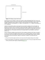
resistance is the shortest one, as shown in Figure 6.6
.

Figure 6.6: Choosing paths based on length alone
Other worlds are not so constant. Resistance factors can be worked into algorithms to account for
something like a room that has the chance of being filled with lava (like the main area of DM2 in Quake).
Even if traveling through the lava room is the shortest of all possible paths using sheer distance, the
most logical path is to avoid the lava room if it made sense. Luckily, once the path finding algorithm is
set up, modifying it to support other kinds of cost besides distance is a fairly trivial task. If other factors
are taken into account, the chosen path may be different. See Figure 6.7
.

286

Figure 6.7: Choosing paths based on other criterion
Groundwork

While there are algorithms for path planning in just about every sort of environment, I'm going to focus
on path planning in networked convex polyhedral cells. Path planning for something like a 2D map (like
those seen in Starcraft) is better planned with algorithms like A*.
A convex cell will be defined as a region of passable space that a creature can wander through, such as
a room or hallway. Convex polyhedrons follow the same rules for convexity as the polygons. For a
polygon (2D) or a polyhedron (3D) to be convex, any ray that is traced between any two points in the
cell cannot leave the cell. Intuitively, the cell cannot have any dents or depressions in it; there isn't any
part of the cell that sticks inward. Concavity is a very important trait for what is being done here. At any
point inside the polyhedron, exiting the polyhedron at any location is possible and there is no need to
worry about bumping into walls. Terminator logic can be used from before until the edge of the
polyhedron is reached.
The polyhedrons, when all laid out, become the world. They do not intersect with each other. They meet
up such that there is exactly one convex polygon joining any two cells. This invisible boundary polygon
is a special type of polygon called a portal. Portals are the doorways connecting rooms and are
passable regions themselves. If you enter and exit cells from portals, and you know a cell is convex,
then you also know that any ray traveled between two portals will not be obstructed by the walls of the
cell (although it may run against a wall). Until objects are introduced into the world, if the paths are
followed exactly, there is no need to perform collision tests.

287

Figure 6.8: Cells and the portals connecting them
I'll touch upon this spatial definition later in the book when I discuss hidden surface removal algorithms;
portal rendering uses this same paradigm to accelerate hidden surface removal tasks.
The big question that remains is how do you move around this map? To accomplish finding the shortest
path between two arbitrary locations on the map (the location of the creature and a location the user
chooses), I'm going to build a directed, weighted graph and use Dijkstra's algorithm to find the shortest
edge traversal of the graph.
If that last sentence didn't make a whole lot of sense, don't worry, just keep reading!
Graph Theory

The need to find the shortest path in graphs shows up everywhere in computer programming. Graphs
can be used to solve a large variety of problems, from finding a good path to send packets through on a
network of computers, to planning airline trips, to generating door-to-door directions using map
software.
A weighted, directed graph is a set of nodes connected to each other by a set of edges. Nodes contain
locations, states you would like to reach, machines, anything of interest. Edges are bridges from one
node to another. (The two nodes being connected can be the same node, although for these purposes
that isn't terribly useful.) Each edge has a value that describes the cost to travel across the edge, and is
unidirectional. To travel from one node to another and back, two edges are needed: one to take you
from the first node to the second, and one that goes from the second node to the first.
Dijkstra's algorithm allows you to take a graph with positive weights on each edge and a starting
location and find the shortest path to all of the other nodes (if they are reachable at all). In this algorithm

288
each node has two pieces of data associated with it: a "parent" node and a "best cost" value. Initially, all
of the parent values for all of the nodes are set to invalid values, and the best cost values are set to
infinity. The start node's best cost is set to zero, and all of the nodes are put into a priority queue that
always removes the element with the lowest cost. Figure 6.9
shows the initial case.

Figure 6.9: Our initial case for the shortest path computation

Note
Notice that the example graphs I'm using seem to have bidirectional edges (edges with
arrows on both sides). These are just meant as shorthand for two unidirectional edges
with the same cost in both directions. In the successive images, gray circles are visited
nodes and dashed lines are parent links.
Iteratively remove the node with the lowest best cost from the queue. Then look at each of its edges. If
the current best cost for the destination node for any of the edges is greater than the current node's cost
plus the edges' cost, then there is a better path to the destination node. Then update the cost of the

destination node and the parent node information, pointing them to the current node. Pseudocode for
the algorithm appears in Listing 6.5
.
Listing 6.5: Pseudocode for Dijkstra's algorithm

struct node
vector< edge > edges
node parent
real cost

struct edge
node dest

289
real cost

while( priority_queue is not empty )
node curr = priority_queue.pop
for( all edges leaving curr )
if( edge.dest.cost > curr.cost + edge.cost )
edge.dest.cost = curr.cost + edge.cost
edge.dest.parent = curr


Let me step through the algorithm so I can show you what happens. In the first iteration, I take the
starting node off the priority queue (since its best cost is zero and the rest are all set to infinity). All of
the destination nodes are currently at infinity, so they get updated, as shown in Figure 6.10
.

Figure 6.10: Aftermath of the first step of Dijkstra's algorithm

Then it all has to be done again. The new node you pull off the priority queue is the top left node, with a
best cost of 8. It updates the top right node and the center node, as shown in Figure 6.11
.

290

Figure 6.11: Step 2
The next node to come off the queue is the bottom right one, with a value of 10. Its only destination
node, the top right one, already has a best cost of 13, which is less than 15 (10 + the cost of the edge
−15). Thus, the top right node doesn't get updated, as shown in Figure 6.12
.

Figure 6.12: Step 3
Next is the top right node. It updates the center node, giving it a new best cost of 14, producing Figure
6.13.

291

Figure 6.13: Step 4
Finally, the center node is visited. It doesn't update anything. This empties the priority queue, giving the
final graph, which appears in Figure 6.14
.

Figure 6.14: The graph with the final parent-pointers and costs
Using Graphs to Find Shortest Paths
Now, armed with Dijkstra's algorithm, you can take a point and find the shortest path and shortest
distance to all other visitable nodes on the graph. But one question remains: How is the graph to
traverse generated? As it turns out, this is a simple, automatic process, thanks to the spatial data
structure.
First, the kind of behavior that you wish the creature to have needs to be established. When a creature's

target exists in the same convex cell the creature is in, the path is simple: Go directly towards the object
using something like the Terminator AI I discussed at the beginning of the chapter. There is no need to
worry about colliding with walls since the definition of convexity assures that it is possible to just march
directly towards the target.

292

Warning
I'm ignoring the fact that the objects take up a certain amount of space, so the total
set of the creature's visitable points is slightly smaller than the total set of points in
the convex cell. For the purposes of what I'm doing here, this is a tolerable problem,
but a more robust application would need to take this fact into account.
So first there needs to be a way to tell which cell an object is in. Luckily, this is easy to do. Each polygon
in a cell has a plane associated with it. All of the planes are defined such that the normal points into the
cell. Simply controlling the winding order of the polygons created does this. Also known is that each
point can be classified whether it is in front of or in back of a plane. For a point to be inside a cell, it must
be in front of all of the planes that make up the boundary of the cell.
It may seem mildly counterintuitive to have the normals sticking in towards the center of the object
rather than outwards, but remember that they're never going to be considered for drawing from the
outside. The cells are areas of empty space surrounded by solid matter. You draw from the inside, and
the normals point towards you when the polygons are visible, so the normals should point inside.
Now you can easily find out the cell in which both the source and destination locations are. If they are in
the same cell, you're done (marching towards the target). If not, more work needs to be done. You need
to generate a path that goes from the source cell to the destination cell. To do this, you put nodes inside
each portal, and throw edges back and forth between all the portals in a cell. An implementation detail is
that a node in a portal is actually held by both of the cells on either side of the portal. Once the network
of nodes is set up, building the edges is fairly easy. Add two edges (one each way) between each of the
nodes in each cell. You have to be careful, as really intricate worlds with lots of portals and lots of nodes
have to be carefully constructed so as not to overload the graph. (Naturally, the more edges in the
graph, the longer Dijkstra's algorithm will take to finish its task.)

You may be wondering why I'm bothering with directed edges. The effect of having two directed edges
going in opposite directions would be the same as having one bi-directed edge, and you would only
have half the edges in the graph. In this 2D example there is little reason to have unidirectional edges.
But in 3D everything changes. If, for example, the cell on the other side of the portal has a floor 20 feet
below the other cell, you can't use the same behavior you use in the 2D example, especially when
incorporating physical properties like gravity. In this case, you would want to let the creature walk off the
ledge and fall 20 feet, but since the creature wouldn't be able to turn around and miraculously leap 20
feet into the air into the cell above, you don't want an edge that would tell you to do so.
Here is where you can start to see a very important fact about AI. Although a creature seems intelligent
now (well… more intelligent than the basic algorithms at the beginning of the chapter would allow), it's
following a very standard algorithm to pursue its target. It has no idea what gravity is, and it has no idea
that it can't leap 20 feet. The intelligence in this example doesn't come from the algorithm itself, but
rather it comes from the implementation, specifically the way the graph is laid out. If it is done poorly (for
example, putting in an edge that told the creature to move forward even though the door was 20 feet

293
above it), the creature will follow the same algorithm it always does but will look much less intelligent
(walking against a wall repeatedly, hoping to magically cross through the doorway 20 feet above it).
Application: Path Planner
The second application for this chapter is a fully functioning path planner and executor. The code loads
a world description off the disk, and builds an internal graph to navigate with. When the user clicks
somewhere in the map, the little creature internally finds the shortest path to that location and then
moves there.
Parsing the world isn't terribly hard; the data is listed in ASCII format (and was entered manually, yuck!).
The first line of the file has one number, providing the number of cells. Following, separated by blank
lines, are that many cells. Each cell has one line of header (containing the number of vertices, number
of edges, number of portals, and number of items). Items were never implemented for this demo, but
they wouldn't be too hard to stick in. It would be nice to be able to put health in the world and tell the
creature "go get health!" and have it go get it.
Points are described with two floating-point coordinates, edges with two indices, and portals with two

indices and a third index corresponding to the cell on the other side of the doorway. Listing 6.6
has a
sample cell from the world file you'll be using.
Listing 6.6: Sample snippet from the cell description file

17

6 5 1 0
-8.0 8.0
-4.0 8.0
-4.0 4.0
-5.5 4.0
-6.5 4.0
-8.0 4.0
0 1
1 2
2 3
4 5
5 0
3 4 8

294

more cells


Building the graph is a little trickier. The way it works is that each pair of doorways (remember, each
conceptual doorway has a doorway structure leading out of both of the cells touching it) holds onto a
node situated in the center of the doorway. Each cell connects all of its doorway nodes together with
dual edges—one going in each direction.

When the user clicks on a location, first the code makes sure that the user clicked inside the boundary
of one of the cells. If it did not, the click is ignored. Only approximate boundary testing is used (using
two-dimensional bounding boxes); more work would need to be done to do more exact hit testing (this is
left as an exercise for the reader).
When the user clicks inside a cell, then the fun starts. Barring the trivial case (the creature and clicked
location are in the same cell), a node is created inside the cell and edges are thrown out to all of the
doorway nodes. Then Dijkstra's algorithm is used to find the shortest path to the node. The shortest
path is inserted into a structure called sPath that is essentially just a stack of nodes. While the creature
is following a path, it peeks at the top of the stack. If it is close enough to it within some epsilon, the
node is popped off the stack and the next one is chosen. When the stack is empty, the creature has
reached its destination.
The application uses the GDI for all the graphics, making it fairly slow. Also, the graph searching
algorithm uses linear searches to find the cheapest node while it's constructing the shortest path. What
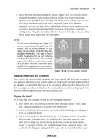
fun would it be if I did all the work for you? A screen shot from the path planner appears in Figure 6.15

on the following page. The creature appears as a red circle.

295

Figure 6.15: Screen shot from the path planner
Listing 6.7
gives the code used to find the shortest path in the graph. There is plenty of other source
code to wander through in this project, but this seemed like the most interesting part.
Listing 6.7: The graph searching code for the path planner


cNode* cWorld::FindCheapestNode()
{
// ideally, we would implement a slightly more advanced
// data structure to hold the nodes, like a heap.

// since our levels are so simple, we can deal with a
// linear algorithm.

float fBestCost = REALLY_BIG;
cNode* pOut = NULL;

296
for( int i=0; i<m_nodeList.size(); i++ )
{
if( !m_nodeList[i]->m_bVisited )
{
if( m_nodeList[i]->m_fCost < fBestCost )
{
// new cheapest node
fBestCost = m_nodeList[i]->m_fCost;
pOut = m_nodeList[i];
}
}
}

// if we haven't found a node yet, something is
// wrong with the graph.
assert( pOut );

return pOut;
}

void cNode::Relax()
{
this->m_bVisited = true;

for( int i=0; i<m_edgeList.size(); i++ )
{
cEdge* pCurr = m_edgeList[i];
if( pCurr->m_fWeight + this->m_fCost < pCurr->m_pTo->m_fCost )
{
// relax the 'to' node
pCurr->m_pTo->m_pPrev = this;
pCurr->m_pTo->m_fCost = pCurr->m_fWeight + this->m_fCost;

297
}
}
}

void cWorld::ShortestPath( sPath* pPath, cNode *pTo, cNode* pFrom )
{
// easy out.
if( pTo == pFrom ) return;

InitShortestPath();

pFrom->m_fCost = 0.f;

bool bDone = false;
cNode* pCurr;
while( 1 )
{
pCurr = FindCheapestNode();
if( !pCurr )

return; // no path can be found.
if( pCurr == pTo )
break; // We found the shortest path

pCurr->Relax(); // relax this node
}

// now we construct the path.

// empty the path first.
while( !pPath->m_nodeStack.empty() ) pPath->m_nodeStack.pop();

pCurr = pTo;

298
while( pCurr != pFrom )
{
pPath->m_nodeStack.push( pCurr );
pCurr = pCurr->m_pPrev;
}
}


Motivation
The final area of AI I'll be discussing is the motivation of a creature. I feel it's the most interesting facet
of AI. The job of the motivation engine is to decide, at a very high level, what the creature should be
doing. Examples of high-level states would be "get health" or "attack nearest player." Once you have
decided on a behavior, you create a set of tasks for the steering engine to accomplish. Using the "get
health" example, the motivation engine would look through an internal map of the world for the closest
health and then direct the locomotion engine to find the shortest path to it and execute the path. I'll show

you a few high-level motivation concepts.
Non-Deterministic Finite Automata (NFAs)
NFAs are popular in simpler artificial intelligence systems (and not only in AI; NFAs are used
everywhere). If, for example, you've ever used a search program like grep (a UNIX searching
command), you've used NFAs. They're a classical piece of theoretic computer science, an extension of
Deterministic Finite Automata (DFAs).
How do they work? In the classic sense, you have a set of nodes connected with edges. One node (or
more) is the start node and one (or more) is the end node. At any point in time, there is a set of active
nodes. You send a string of data into an NFA. Each piece is processed individually.
The processing goes as follows: Each active node receives the current piece of data. It makes itself
inactive and compares the data to each of its edges. If any of its outgoing edges match the input data,
they turn their destination node on. There is a special type of edge called an epsilon edge, which turns
its destination on regardless of the input.
When all of the data has been processed, you look at the list of active nodes. If any of the end nodes
are active, then that means the string of data passed. You construct the NFA to accept certain types of
strings and can quickly run a string through an NFA to test it.
Here are a few examples to help make the definition more concrete. Both of the examples are fairly
simple NFAs just to show the concepts being explained. Let's say there is an alphabet with exactly two

299
values, A and B. The first example, Figure 6.16
, is an NFA that accepts only the string ABB and nothing
else.

Figure 6.16: NFA that accepts the string ABB
The second example, Figure 6.17
, shows an NFA that accepts the string A*B, where A* means any
number of As, including zero.

Figure 6.17: NFA that accepts the string A*B

How is this useful for game programming? If you encode the environment that the creature exists in into
a string that you feed into an NFA, you can allow it to process its scene and decide what to do. You
could have one goal state for each of the possible behaviors (that is, one for "attack enemy," one for

300
"get health," and other high-level behaviors). As an example, one of the entries in the array of NFA data
could represent how much ammo the character has. Let's say there are three possible states: {Plenty of
ammo, Ammo, Little or no ammo}. The edge that corresponded to "Plenty of ammo" would lead to a
section of the NFA that would contain aggressive end states, while the "Little or no ammo" edges would
lead to a section of the NFA that would most likely have the creature decide that it needed to get some
ammo. The next piece of data would describe a different aspect of the universe the creature existed in,
and the NFA would have branches ready to accept it.
Table 6.1
contains some examples of states that could be encoded in the string of data for the NFA.


Table 6.1: Some example states that could be encoded into an NFA
Proximity to
nearest
opponent
Very near; Average distance; Very far.
If the nearest opponent is very far, the edge could lead to states that encourage
the collection of items.

Health Plenty of health; Adequate health; Dangerous health.
If the creature has dangerously low health and the opponent was very near, a
kamikaze attack would probably be in order. If the nearest enemy was very far
away, it should consider getting some health.

Environment Tight and close; Medium; Expansive.

A state like this would determine which weapon to use. For example, an
explosive weapon like a rocket launcher shouldn't be used in tight and close
areas.

Enemy health Plenty of health; Adequate health; Dangerous health.
The health of the nearest enemy determines the attacking pattern of the
creature. Even if the creature has moderate to low health, it should try for the
kill if the enemy has dangerous health.

Enemy altitude Above; Equal; Below.
It's advantageous in most games to be on higher ground than your opponent,
especially in games with rocket launcher splash damage. If the creature is
below its nearest opponent and the opponent is nearby, it might consider
retreating to higher ground before attacking.

301

One way to implement NFAs would be to have a function pointer in each end state that got executed
after the NFA was processed if the end state succeeded.
The only problem with NFAs is that it's extremely difficult to encode fuzzy decisions. For example, it
would be better if the creature's health was represented with a floating-point value, so there would be a
nearly continuous range of responses based on health. I'll show you how to use neural networks to do
this. However, NFA-based AI can be more than adequate for many games. If your NFA's behavior is too
simple, you generally only need to extend the NFA, adding more behaviors and more states.
Genetic Algorithms
While not directly a motivation concept, genetic algorithms (or GAs) can be used to tweak other
motivation engines. They try to imitate nature to solve problems. Typically, when you're trying to solve a
problem that has a fuzzy solution (like, for example, the skill of an AI opponent), it's very hard to tweak
the numbers to get the best answer.
One way to solve a problem like this is to attack it the way nature does. In nature (according to Darwin,

anyway) animals do everything they can to survive long enough to produce offspring. Typically, the only
members of a species that survive long enough to procreate are the most superior of their immediate
peers. In a pride of lions, only one male impregnates all of the females. All of the other male lions vie for
control of the pride, so that their genes get carried on.
Added to this system, occasionally, is a bit of mutation. An offspring is the combination of the genes of
the two parents, but it may be different from either of the parents by themselves. Occasionally, an
animal will be born with bigger teeth, sharper claws, longer legs, or in Simpsonian cases, a third eye.
The change might give that particular offspring an advantage over its peers. If it does, that offspring is
more likely than the other animals to carry on its genes, and thus, over time, the species improves.
That's nice and all, but what does that have to do with software development? A lot, frankly. What if you
could codify the parameters of a problem into genes? You could randomly create a set of animals, each
with its own genes. They are set loose, they wreak havoc, and a superior pair of genes is found. Then
you combine these two genes, sprinkle some random perturbations in, and repeat the process with the
new offspring and another bunch of random creatures.
For example, you could define the behavior of all the creatures in terms of a set of scalar values. Values
that define how timid a creature is when it's damaged, how prone it is to change its current goal, how
accurate its shots are when it is moving backward, and so forth. Correctly determining the best set of
parameters for each of the creatures can prove difficult. Things get worse when you consider other
types of variables, like the weapon the creature is using and the type of enemy it's up against.

302
Genetic algorithms to the rescue! Initially, you create a slew of creatures with a bunch of random values
for each of the parameters and put them into a virtual battleground, having them duke it out until only
two creatures remain. Those two creatures mate, combining their genes and sprinkling in a bit of
mutation to create a whole new set of creatures, and the cycle repeats.
The behavior that genetic algorithms exhibit is called hill climbing. You can think of a creature's
idealness as a function of n variables. The graph for this function would have many relative maximums
and one absolute maximum. In the case where there were only two variables, you would see a graph
with a bunch of hills (where the two parameters made a formidable opponent), a bunch of valleys
(where the parameters made a bad opponent), and an absolute maximum (the top of the tallest

mountain: the best possible creature).
For each iteration, the creature that will survive will hopefully be the one that was the highest on the
graph. Then the iteration continues, with a small mutation (you can think of this as sampling the area
immediately around the creature). The winner of the next round will be a little bit better than its parent as
it climbs the hill. When the children stop getting better, you know you have reached the top of a hill, a
relative maximum.
How do you know if you reached the absolute maximum, the tallest hill on the graph? It's extremely hard
to do. If you increase the amount of mutation, you increase the area you sample around the creature, so
you're more likely to happen to hit a point along the slope of the tallest mountain. However, the more
you increase the sampling area, the less likely you are to birth a creature further up the mountain, so the
function takes much longer to converge.
Rule-Based AI
The world of reality is governed by a set of rules, rules that control everything from the rising and setting
of the sun to the way cars work. The AI algorithms discussed up to this point aren't aware of any rules,
so they would have a lot of difficulty knowing how to start a car, for example.
Rule-based AI can help alleviate this problem. You define a set of rules that govern how things work in
the world. The creature can analyze the set of rules to decide what to do. For example, let's say that a
creature needs health. It knows that there is health in a certain room, but to get into the room the
creature must open the door, which can only be done from a security station console. One way to
implement this would be to hardcode the knowledge into the creature. It would run to the security
station, open the door, run through it, and grab the health.
However, a generic solution has a lot of advantages. The behavior it can exhibit isn't limited to just
opening security doors. Anything you can describe with a set of rules is something it can figure out. See
Listing 6.8
for a subset of the rules for a certain world.
Listing 6.8: Some rules for an example world

303

IF [Health_Room == Visitable]

THEN [Health == Gettable]
IF [Security_Door == Door_Open]
THEN [Health_Room == Visitable]
IF [Today == Sunday]
THEN [Tacos == 0.49]
IF [Creature_Health < 0.25]
THEN [Creature_State = FindGettableHealth]
IF [Creature_Position NEAR Security_Console]
THEN [Security_Console_Usable]
IF [Security_Console_Usable] AND [Security_Door != Door_Open]
THEN [Creature_Use(Security_Console)]
IF [Security_Console_Used]
THEN [Security_Door == Door_Open]
IF [Creature_Move_To(Security_Console)]
THEN [Creature_Position NEAR Security_Console]


Half the challenge in setting up rule-based systems is to come up with an efficient way to encode the
rules. The other half is actually creating the rules. Luckily a lot of the rules, like the Creature_Move_To
rule at the end of the list, can be automatically generated.
How does the creature figure out what to do, given these rules? It has a goal in mind: getting health. It
looks in the rules and finds the goal it wants, [Health == Gettable]. It then needs to satisfy the condition
for that goal to be true, that is [Health_Room == Visitable]. The creature can query the game engine and
ask it if the health room is visitable. When the creature finds out that it is not, it has a new goal: making
the health room visitable.
Searching the rules again, it finds that [Health_Room == Visitable] if [Security_Door == Door_Open].
Once again, it sees that the security door is not open, so it analyzes the rule set again, looking for a way
to satisfy the condition.
This process continues until the creature reaches the rule saying that if it moves to the security console,
it will be near the security console. Finally, a command that it can do! It then uses path planning to get

304
to the security console, presses the button to open the security door, moves to the health room, and
picks up the health.
AI like this can be amazingly neat. Nowhere do you tell how to get the health. It actually figured out how
to do it all by itself. If you could encode all the rules necessary to do anything in a particular world, then
the AI would be able to figure out how to accomplish whatever goals it wanted. The only tricky thing is
encoding this information in an efficient way. And if you think that's tricky, try getting the creature to
develop its own rules as it goes along. If you can get that, your AI will always be learning, always
improving.
Neural Networks
One of the huge areas of research in AI is in neural networks (NNs). They take a very fundamental
approach to the problem of artificial intelligence by trying to closely simulate intelligence, in the physical
sense.
Years of research have gone into studying how the brain actually works (it's mystifying that evolution
managed to design an intelligence capable of analyzing itself). Researchers have discovered the basic
building blocks of the brain and have found that, at a biological level, it is just a really, really (REALLY)
dense graph. On the order of billions or trillions of nodes, and each node is connected to thousands of
others.
The difference between the brain and other types of graphs is that the brain is extremely connected.
Thinking of several concepts brings up several other concepts, simply through the fact that the nodes
are connected. As an example, think for a moment about an object that is leafy, green, and crunchy.
You most likely thought about several things, maybe celery or some other vegetable. That's because
there is a strong connection between the leafy part of your brain and things that are leafy. When the
leafy neuron fires, it sends its signal to all the nodes it's connected to. The same goes for green and
crunchy. Since, when you think of those things, they all fire and all send signals to nodes, some nodes
receive enough energy to fire themselves, such as the celery node.
Now, I'm not going to attempt to model the brain itself, but you can learn from it and build your own
network of electronic neurons. Graphs that simulate brain activity in this way are generally called neural
networks.

Neural networks are still a very active area of research. In the last year or so, a team was able to use a
new type of neural network to understand garbled human speech better than humans can! One of the
big advantages of neural networks is that they can be trained to remember their past actions. You can
teach them, giving them an input and then telling them the correct output. Do this enough times and the
network can learn what the correct answer is.

305
However, that is a big piece of pie to bite down on. Instead, I'm going to delve into a higher-level
discussion of neural networks, by explaining how they work sans training, and providing code for you to
play with.
A Basic Neuron
Think of a generic neuron in your brain as consisting of three biological parts: an axon, dendrites, and a
soma. The processing unit is the soma. It takes input coming from the dendrites and outputs to the
axon. The axon, in turn, is connected to the dendrites of other neurons, passing the signals on. These
processes are all handled with chemicals in real neurons; a soma that fires is, in essence, sending a
chemical down its axon that will meet up with other dendrites, sending the fired message to other
neurons. Figure 6.18
shows what a real neuron looks like.

Figure 6.18: A biological neuron
The digital version is very similar. There is a network of nodes connected by edges. When a node is
processed, it takes all of the signals on the incoming edges and adds them together. One of these
edges is a special bias or memory edge, which is just an edge that is always on. This value can change
to modify the behavior of the network (the higher the bias value, the more likely the neuron is to fire). If
the summation of the inputting nodes is above the threshold (usually 1.0), then the node sends a fire
signal to each of its outgoing edges. The fire signal is not the result of the addition, as that may be much
more than 1.0. It is always 1.0. Each edge also has a bias that can scale the signal being passed it
higher or lower. Because of this, the input that arrives at a neuron can be just about any value, not just
1.0 (firing neurons) or 0 (non-firing neurons). They may be anywhere; if the edge bias was 5.0, for
example, the neuron would receive 5.0 or 0, depending on whether the neuron attached to it fired or

not. Using a bias on the edges can also make a fired neuron have a dampened effect on other neurons.
The equation for the output of a neuron can be formalized as follows:

306

where you sum over the inputs n (the bias of the edge, multiplied by the output of the neuron attached
to it) plus the weight of the bias node times the bias edge weight.
Other types of responses to the inputs are possible; some systems use a Sigmoid exponential function
like the one below. A continuous function such as this makes it easier to train certain types of networks
(back propagation networks, for example), but for these purposes the all-or-nothing response will do the
job.

One of the capabilities of the brain is the ability to imagine things given a few inputs. Imagine you hear
the phrases "vegetable," "orange," and "eaten by rabbits." Your mind's eye conjures up an image of
carrots. Imagine your neural network's inputs are these words and your outputs are names of different
objects. When you hear the word "orange," somewhere in your network (and your brain) an "orange"
neuron fires. It sends a fire signal to objects you have associated with the word "orange" (for example:
carrots, oranges, orange crayons, an orange shirt). That signal alone probably won't be enough for any
particular one of those other neurons to fire; they need other signals to help bring the total over the
threshold. If you then hear another phrase, such as "eaten by rabbits," the "eaten by rabbits" neuron will
fire off a signal to all the nodes associated with that word (for example: carrots, lettuce, boisterous
English crusaders). Those two signals may be enough to have the neuron fire, sending an output of
carrots. Figure 6.19
abstractly shows what is happening.


307
Figure 6.19: A subsection of a hypothetical neural network
Simple Neural Networks
Neural networks are Turing-complete; that is, they can be used to perform any calculation that

computers can do, given enough nodes and enough edges. Given that you can construct any processor
using nothing but NAND gates, this doesn't seem like too ridiculous a conjecture. Let's look at some
simpler neural networks before trying to tackle anything more complex.
AND
Binary logic seems like a good place to start. As a first stab at a neural net, let's try to design a neural
net that can perform a binary AND. The network appears in Figure 6.20
.

Figure 6.20: A neural network that can perform a binary AND function
Note that the input nodes have a bias of 0.1. This is to help fuzzify the numbers a bit. You could make
the network strict if you'd like (setting the bias to 0.0), but for many applications 0.9 is close enough to
1.0 to count as being 1.0.
OR
Binary OR is similar to AND; the middle edges just have a higher weight so that either one of them can
activate the output node. The net appears in Figure 6.21
.

308

Figure 6.21: A neural network that can perform a binary OR function
XOR
Handling XOR requires a bit more thought. Three nodes alone can't possibly handle XOR; you need to
make another layer to the network. A semi-intuitive reasoning behind the workings of Figure 6.22
: The
top internal node will only be activated if both input nodes fire. The bottom one will fire if either of the
input nodes fires. If both internal nodes fire, that means that both input nodes fired (a case you should
not accept), which is correctly handled by having a large negative weight for the edge leading from the
top internal node to the output node.

Figure 6.22: A neural network that can perform a binary XOR function

Training Neural Networks
While it's outside the scope of this book, it's important to know one of the most important and interesting
features about neural nets: They can be trained. Suppose you create a neural net to solve a certain

309
problem (or put another way, to give a certain output given a set of inputs). You can initially seed the
network with random values for all of the edge biases and then have the network learn. Neural nets can
be trained or can learn autonomously. An autonomously learning neural net would be, for example, an
AI that was trying to escape from a maze. As it moves, it learns more information, but it has no way to
check its answer as it goes along. These types of networks learn much slower than trained networks.
Trained neural networks on the other hand have a cheat sheet; that is, they know the solution to each
problem. They run an input and check their output against the correct answer. If it is wrong, the network
modifies some of the weights so that it gets the correct answer the next time.
Using Neural Networks in Games
Using a neural network to decide the high-level action to perform in lieu of NFAs has a lot of
advantages. For example, the solutions are often much fuzzier. Reaching a certain state isn't as black
and white as achieving a certain value in the string of inputs; it's the sum of a set of factors that all
contribute to the behavior.
As an example, let's say that you have a state that, when reached, causes your creature to flee its
current location in search of health. You may want to do this in many cases. One example would be if
there was a strong enemy nearby. Another would be if there was a mildly strong enemy nearby and the
main character is low on health. You can probably conjure up a dozen other cases that would justify
turning tail and fleeing.
While it's possible to codify all of these cases separately into an NFA, it's rather tedious. It's better to
have all of the input states (proximity of nearest enemy, strength of nearest enemy, health, ammo, etc.)
become inputs into the neural network. Then you could just have an output node that, when fired,
caused the creature to run for health. This way, the behavior emerges from the millions of different
combinations for inputs. If enough factors contribute to the turn-and-flee state to make it fire, it will sum
over the threshold and fire.
A neural network that does this is exactly what I'm going to show you how to write.

Application: NeuralNet
The NeuralNet sample application is a command-line application to show off a neural network simulator.
The network is loaded off disk from a description file; input values for the network are requested from
the user, then the network is run and the output appears on the console. I'll also build a sample network
that simulates a simple creature AI. An example running of the network appears in Listing 6.9
. In this
example, the creature has low health, plenty of ammo, and an enemy nearby. The network decides to
select the state [Flee_Enemy_ Towards_Health]. If this code were to be used in a game, state-setting
functions would be called in lieu of printing out the names of the output states.
Listing 6.9: Sample output of the neural net simulator