Điều khiển kết cấu - Chương 1 ppt
Bạn đang xem bản rút gọn của tài liệu. Xem và tải ngay bản đầy đủ của tài liệu tại đây (225.6 KB, 44 trang )
1
Chapter 1
Introduction
1.1 Motivation for structural motion control
Limitations of conventional structural design
The word, design, has two meanings. When used as a verb it is defined as the act
of creating a description of an artifact. It is also used as a noun, and in this case, is
defined as the output of the activity, i.e., the description. In this text, structural
design is considered to be the activity involved in defining the physical makeup
of the structural system. In general, the “designed” structure has to satisfy a set of
requirements pertaining to safety and serviceability. Safety relates to extreme
loadings which are likely to occur no more than once during a structure’s life. The
concerns here are the collapse of the structure, major damage to the structure and
its contents, and loss of life. Serviceability pertains to moderate loadings which
may occur several times during the structure’s lifetime. For service loadings, the
structure should remain fully operational, i.e. the structure should suffer
negligible damage, and furthermore, the motion experienced by the structure
should not exceed specified comfort limits for humans and motion sensitive
equipment mounted on the structure. An example of a human comfort limit is the
restriction on the acceleration; humans begin to feel uncomfortable when the
acceleration reaches about . A comprehensive discussion of human comfort0.02g
2 Chapter 1: Introduction
criteria is given by Bachmann and Ammann (1987).
Safety concerns are satisfied by requiring the resistance (i.e. strength) of the
individual structural elements to be greater than the demand associated with the
extreme loading. The conventional structural design process proportions the
structure based on strength requirements, establishes the corresponding stiffness
properties, and then checks the various serviceability constraints such as elastic
behavior. Iteration is usually necessary for convergence to an acceptable
structural design. This approach is referred to as strength based design since the
elements are proportioned according to strength requirements.
Applying a strength based approach for preliminary design is appropriate
when strength is the dominant design requirement. In the past, most structural
design problems have fallen in this category. However, a number of
developments have occurred recently which have limited the effectiveness of the
strength based approach.
Firstly, the trend toward more flexible structures such as tall buildings and
longer span horizontal structures has resulted in more structural motion under
service loading, thus shifting the emphasis from safety toward serviceability. For
instance, the wind induced lateral deflection of the Empire State Building in New
York City, one of the earliest tall buildings in the United States, is several inches
whereas the wind induced lateral deflection of the World Trade Center tower is
several feet, an order of magnitude increase. This difference is due mainly to the
increased height and slenderness of the World Trade Center in comparison to the
Empire State tower. Furthermore, satisfying the limitation on acceleration is a
difficult design problem for tall slender buildings.
Secondly, some of the new types of facilities such as space platforms and
semi-conductor manufacturing centers have more severe design constraints on
motion than the typical civil structure. In the case of microdevice manufacturing,
the environment has to be essentially motion free. Space platforms used to
support mirrors have to maintain a certain shape to a small tolerance in order for
the mirror to properly function. The design strategy for motion sensitive structures
is to proportion the members based on the stiffness needed to satisfy the motion
constraints, and then check if the strength requirements are satisfied.
Thirdly, recent advances in material science and engineering have resulted
in significant increases in the strength of traditional civil engineering materials
1.1 Motivation for Structural Motion Control 3
such as steel and concrete, as well as a new generation of composite materials.
Although the strength of structural steel has essentially doubled, its elastic
modulus has remained constant. Also, there has been some increase in the elastic
modulus for concrete, but this improvement is still small in comparison to the
increment in strength. The lag in material stiffness versus material strength has
led to a problem with satisfying the serviceability requirements on the various
motion parameters. Indeed, for very high strength materials, it is possible for the
serviceability requirements to be dominant. Some examples presented in the
following sections illustrate this point.
Motion based structural design and motion control
Motion based structural design is an alternate design process which is
more effective for the structural design problem described above. This approach
takes as its primary objective the satisfaction of motion related design
requirements, and views strength as a constraint, not as a primary requirement.
Motion based structural design employs structural motion control methods to
deal with motion issues. Structural motion control is an emerging engineering
discipline concerned with the broad range of issues associated with the motion of
structural systems such as the specification of motion requirements governed by
human and equipment comfort, and the use of energy storage, dissipation, and
absorption devices to control the motion generated by design loadings. Structural
motion control provides the conceptional framework for the design of structural
systems where motion is the dominant design consideration. Generally, one seeks
the optimal deployment of material and motion control mechanisms to achieve
the design targets on motion as well as satisfy the constraints on strength.
In what follows, a series of examples which reinforce the need for an
alternate design paradigm having motion rather than strength as its primary
focus, and illustrate the application of structural motion control methods to
simple structures is presented. The first three examples deal with the issue of
strength versus serviceability from a static perspective for building type
structures. The discussion then shifts to the dynamic regime. A single-degree-of-
freedom (SDOF) system is used to introduce the strategy for handling motion
constraints for dynamic excitation. The last example extends the discussion
further to multi-degree-of-freedom (MDOF) systems, and illustrates how to deal
with one of the key issues of structural motion control, determining the optimal
stiffness distribution. Following the examples, an overview of structural motion
control methodology is presented.
4 Chapter 1: Introduction
1.2 Motion versus strength issues for building type structures
Building configurations have to simultaneously satisfy the requirements of site
(location and geometry), building functionality (occupancy needs), appearance,
and economics. These requirements significantly influence the choice of the
structural system and the corresponding design loads. Buildings are subjected to
two types of loadings: gravity loads consisting of the actual weight of the structural
system and the material, equipment, and people contained in the building, and
lateral loads consisting mainly of wind and earthquake loads. Both wind and
earthquake loadings are dynamic in nature and produce significant amplification
over their static counterpart. The relative importance of wind versus earthquake
depends on the site location, building height, and structural makeup. For steel
buildings, the transition from earthquake dominant to wind dominant loading for a
seismically active region occurs when the building height reaches approximately
. Concrete buildings, because of their larger mass, are controlled by
earthquake loading up to at least a height of , since the additional gravity
load increases the seismic forces. In regions where the earthquake action is low
(e.g. Chicago in the USA), the transition occurs at a much lower height, and the
design is governed primarily by wind loading.
When a low rise building is designed for gravity loads, it is very likely that
the underlying structure can carry most of the lateral loads. As the building
height increases, the overturning moment and lateral deflection resulting from
the lateral loads increase rapidly, requiring additional material over and above
that needed for the gravity loads alone. Figure 1.1 (Taranath, 1988) illustrates how
the unit weight of the structural steel required for the different loadings varies
with the number of floors. There is a substantial weight cost associated with
lateral loading.
100m
250m
1.2 Motion Versus Strength Issues for Building Type Structure 5
Fig. 1.1: Structural steel quantities for gravity and wind systems
To illustrate the dominance of motion over strength as the slenderness of
the structure increases, the uniform cantilever beam shown in Fig. 1.2 is
considered. The lateral load is taken as a concentrated force applied to the tip of
the beam, and is assumed to be static. The limiting cases of a pure shear beam and
a pure bending beam are examined.
Fig. 1.2: Building modeled as a uniform cantilever beam
0 50 100 150 200 250
0
20
40
60
80
100
120
140
Gravity loads Lateral loads
Floor Columns
Number of floors
500
1000
Structural steel - N/m
2
1500
2000
2500
p
H
d
w
aa
p
u
d
section a-a
6 Chapter 1: Introduction
Example 1.1: Cantilever shear beam
The shear stress is given by
(1.1)
where is the cross sectional area over which the shear stress can be considered
to be constant. When the bending rigidity is very large, the displacement, , at
the tip of the beam is due mainly to shear deformation, and can be estimated as
(1.2)
where is the shear modulus and is the height of the beam. This model is
called a shear beam. The shear area needed to satisfy the strength requirement
follows from eqn (1.1):
(1.3)
where is the allowable stress. Noting eqn (1.2), the shear area needed to satisfy
the serviceability requirement on displacement is
(1.4)
where denotes the allowable displacement. The ratio of the area required to
satisfy serviceability to the area required to satisfy strength provides an estimate
of the relative importance of the motion design constraints versus the strength
design constraints
(1.5)
Figure 1.3 shows the variation of r with . Increasing places
τ
τ
p
A
s
=
A
s
u
u
pH
GA
s
=
GH
A
s
strength
p
τ
∗
≥
τ
∗
A
s
serviceability
p
G
H
u
∗
⋅≥
u
∗
r
A
s
serviceability
A
s
strength
τ
∗
G
H
u
∗
⋅==
Hu
∗
⁄ Hu
∗
⁄
1.2 Motion Versus Strength Issues for Building Type Structure 7
more emphasis on the motion constraint since it corresponds to a decrease in the
allowable displacement, . Furthermore, an increase in the allowable shear
stress, , also increases the dominance of the displacement constraint.
Fig. 1.3: Plot of versus for a pure shear beam
Example 1.2: Cantilever bending beam
When the shear rigidity is very large, shear deformation is negligible, and the
beam is called a “bending” beam. The maximum bending moment in the
structure occurs at the base and equals
(1.6)
The resulting maximum stress is
(1.7)
where is the section modulus, is the moment of inertia of the cross-section
about the bending axis, and is the depth of the cross-section (see Fig. 1.2). The
corresponding displacement at the tip of the beam becomes
u
∗
τ
∗
200 300 400100
H
u
∗
r
τ
1
*
τ
2
*
τ
1
*
>
rHu
∗
⁄
M
MpH=
σ
σ
M
S
Md
2I
pHd
2I
== =
SI
d
u
8 Chapter 1: Introduction
(1.8)
The moment of inertia needed to satisfy the strength requirement is given by
(1.9)
Using eqn (1.8), the moment of inertia needed to satisfy the serviceability
requirement is
(1.10)
Here, and denote the allowable displacement and stress respectively. The
ratio of the moment of inertia required to satisfy serviceability to the moment of
inertia required to satisfy strength has the form
(1.11)
Figure 1.4 shows the variation of with for a constant value of the
aspect ratio ( for tall buildings). Similar to the case of the shear
beam, an increase in places more emphasis on the displacement since it
corresponds to a decrease in the allowable displacement, , for a constant .
Also, an increase in the allowable stress, , increases the importance of the
displacement constraint.
For example, consider a standard strength steel beam with an allowable
stress of , a modulus of elasticity of , and an
aspect ratio of . The value of at which a transition from strength
to serviceability occurs is
(1.12)
For , and motion controls the design. On the other hand, if high
u
pH
3
3EI
=
I
strength
pHd
2σ
∗
≥
I
serviceability
pH
3
3Eu
∗
≥
u
∗
σ
∗
r
I
serviceability
I
strength
pH
3
3Eu
∗
2σ
∗
pHd
⋅
2H
3d
σ
∗
E
H
u
∗
⋅⋅===
rHu
∗
⁄
Hd⁄ Hd⁄ 7≈
Hu
∗
⁄
u
∗
H
σ
∗
σ
∗
200MPa= E 200,000MPa=
Hd⁄ 7= Hu
∗
⁄
H
u
∗
r 1=
3
2
E
σ
∗
d
H
200≈⋅⋅=
Hu
∗
⁄ 200> r 1>
1.2 Motion Versus Strength Issues for Building Type Structure 9
strength steel is utilized ( and )
(1.13)
and motion essentially controls the design for the full range of allowable
displacement.
Fig. 1.4: Plot of versus for a pure bending beam
Example 1.3: Quasi-shear beam frame
This example compares strength vs. motion based design for a single bay frame of
height and load (see Fig. 1.5). For simplicity, a very stiff girder is assumed,
resulting in a frame that displays quasi-shear beam behavior. Furthermore, the
columns are considered to be identical, each characterized by a modulus of
elasticity , and a moment of inertia about the bending axis .
The maximum moment, , in each column is equal to
(1.14)
σ
∗
400MPa= E 200,000MPa=
H
u
∗
r 1=
100≈
200 300 400100
H
u
∗
r
σ
1
*
σ
2
*
σ
1
*
>
rHu
∗
⁄
Hp
E
c
I
c
M
M
pH
4
=
10 Chapter 1: Introduction
The lateral displacement of the frame under the load is expressed as
Fig. 1.5: Quasi-shear beam example
(1.15)
where denotes the equivalent shear rigidity which, for this structure, is given
by
(1.16)
The strength constraint requires that the maximum stress in the column be
less than the allowable stress
(1.17)
where represents the depth of the column in the bending plane. Equation (1.17)
is written as
(1.18)
The serviceability requirement constrains the maximum displacement to
be less than the allowable displacement
u
H
E
c
, I
c
E
c
, I
c
I
g
∞=
p
2
p
2
u
pH
D
T
=
D
T
D
T
24E
c
I
c
H
2
=
σ
∗
Md
2I
c
pHd
8I
c
σ
∗
≤=
d
I
c
strength
pHd
8σ
∗
≥
u
∗
1.3 Design of a Single-degree-of Freedom System for Dynamic Loading 11
(1.19)
The corresponding requirement for is
(1.20)
Forming the ratio of the moment of inertia required to satisfy the serviceability
requirement to the moment of inertia required to satisfy the strength requirement,
(1.21)
leads to the value of for which motion dominates the design
(1.22)
1.3 Design of a single-degree-of freedom system for dynamic loading
The previous examples dealt with motion based design for static loading. A
similar approach applies for dynamic loading once the relationship between the
excitation and the response is established. The procedure is illustrated for the
single-degree-of-freedom (SDOF) system shown in Fig. 1.6.
Response for periodic excitation
The governing equation of motion of the system has the form
(1.23)
pH
3
24E
c
I
c
u
∗
≤
I
c
I
c
serviceability
pH
3
24E
c
u
∗
≥
r
I
c
serviceability
I
c
strength
σ
∗
3E
c
H
d
H
u
∗
⋅⋅==
Hu
∗
⁄
H
u
∗
3E
c
σ
∗
d
H
⋅≥
mu
˙˙
t() cu
˙
t() ku t()++ pt()=
12 Chapter 1: Introduction
Fig. 1.6: Single-degree-of-freedom system
where , , are the mass, stiffness, and viscous damping parameters of the
system respectively, is the applied loading, is the displacement, and is the
independent time variable. The dot operator denotes differentiation with respect
to time. Of interest is the case where is a periodic function of time. Taking to
be sinusoidal in time with frequency ,
(1.24)
the corresponding forced vibration response is given by
(1.25)
where and characterize the response. They are related to the system and
loading parameters as follows:
(1.26)
(1.27)
(1.28)
(1.29)
k
c
m
u
p
R
mkc
pu t
pp
Ω
pt() p
ˆ
Ωtsin=
ut() u
ˆ
Ωt δ–()sin=
u
ˆ
δ
u
ˆ
p
ˆ
k
H
1
=
H
1
1
1 ρ
2
–[]
2
2ξρ[]
2
+
=
ω
k
m
=
ξ
c
2ωm
c
2 km
==
1.3 Design of a Single-degree-of Freedom System for Dynamic Loading 13
(1.30)
(1.31)
The term is the displacement response that would occur if the loading
were applied statically; represents the effect of the time varying nature of the
response. Figure 1.7 shows the variation of with the frequency ratio, , for
various levels of damping. The maximum value of and corresponding
frequency ratio are related to the damping ratio by
(1.32)
Fig. 1.7: Plot of versus and
(1.33)
ρ
Ω
ω
Ω
m
k
==
δtan
2ξρ
1 ρ
2
–
=
p
ˆ
k⁄
H
1
H
1
ρ
H
1
ξ
H
1
max
1
2ξ 1 ξ
2
–
=
0 0.2 0.4 0.6 0.8 1 1.2 1.4 1.6 1.8 2
0
0.5
1
1.5
2
2.5
3
3.5
4
4.5
5
ρ
Ω
ω
Ω
m
k
==
H
1
ξ 0.0=
ξ 0.2=
ξ 0.4=
H
1
ρξ
ρ
max
12ξ
2
–=
14 Chapter 1: Introduction
When ,
(1.34)
(1.35)
Since is usually small, the maximum dynamic response is significantly greater
than the static response and is close to 1. For example, for which
corresponds to a high level of damping, the peak response is
(1.36)
(1.37)
When the forcing frequency, , is close to the natural frequency, , the
response is controlled by adjusting the damping. Outside of this region, damping
has less influence, and has essentially no effect for and .
Differentiating twice with respect to time leads to the acceleration, ,
(1.38)
Noting eqn (1.26), the magnitude of can be written as
(1.39)
where
(1.40)
The variation of with for different damping ratios is shown in Fig. 1.8. Note
that the behavior of for small and large is opposite to . The maximum
value of is the same as the maximum value for , but the location (i.e. the
corresponding value of ) is different. They are related to by
ξ
2
<< 1
ρ
max
1≈
H
1
max
1
2ξ
≈
ξ
ρ
max
ξ 0.2=
H
1
max
2.55≈
ρ
max
0.96=
Ωω
ρ 0.4<ρ1.6>
ua
at() u
˙˙
t() Ω
2
u
ˆ
Ωt δ–()sin– a
ˆ
Ωt δ–()sin–== =
a
a
ˆ
p
ˆ
k
Ω
2
H
1
p
ˆ
m
H
2
==
H
2
ρ
2
H
1
ρ
4
1 ρ
2
–[]
2
2ξρ[]
2
+
==
H
2
ρ
H
2
ρ H
1
H
2
H
1
ρξ
1.3 Design of a Single-degree-of Freedom System for Dynamic Loading 15
(1.41)
(1.42)
The ratio is the acceleration the mass would experience if it were
unrestrained and subjected to a constant force of magnitude . One can interpret
as a modification factor which takes into account the time varying nature of
the loading and the system restraints associated with stiffness and damping.
Fig. 1.8: Plot of versus and
Once the system and loading are defined (i.e. , , , , and are
specified), one determines and computes the peak amplitudes using the
following relations
(1.43)
(1.44)
ρ
max
1
12ξ
2
–
=
H
2
max
1
2ξ 1 ξ
2
–
=
p
ˆ
m⁄
p
ˆ
H
2
0 0.2 0.4 0.6 0.8 1 1.2 1.4 1.6 1.8 2
0
0.5
1
1.5
2
2.5
3
3.5
4
4.5
5
ρ
Ω
ω
Ω
m
k
==
H
2
ξ 0.0=
ξ 0.2=
ξ
1
2
=
H
2
ρξ
mkc p
ˆ
Ω
H
1
u
ˆ
p
ˆ
k
H
1
=
a
ˆ
Ω
2
u
ˆ
=
16 Chapter 1: Introduction
(1.45)
Note that for periodic response, the acceleration is related to the displacement by
the square of the forcing frequency. One can also work with instead of .
Design criteria
The design problem differs from analysis in that one starts with the mass of
the system, , and the loading characteristics, and , and determines and
such that the motion parameters, and , satisfy the specified criteria. In general,
one has limits on both displacement and acceleration
(1.46)
(1.47)
where and are the target design values. In this case, since and are
related by
(1.48)
one needs to determine which constraint controls. If , the acceleration
limit controls and the optimal solution will be
(1.49)
(1.50)
If, on the other hand, , the displacement limit controls. For this case, the
optimal solution satisfies
(1.51)
(1.52)
In what follows, both cases are illustrated.
H
1
H
1
Ω mkc,,,()H
1
ρξ,()==
H
2
H
1
mp
ˆ
Ω kc
u
ˆ
a
ˆ
u
ˆ
u
∗
≤
a
ˆ
a
∗
≤
u
∗
a
∗
u
ˆ
a
ˆ
a
ˆ
Ω
2
u
ˆ
=
a
∗
Ω
2
u
∗
≤
u
ˆ
a
∗
Ω
2
u
∗
<=
a
ˆ
a
∗
=
a
∗
Ω
2
u
∗
≥
u
ˆ
u
∗
=
a
ˆ
Ω
2
u
∗
a
∗
<=
1.3 Design of a Single-degree-of Freedom System for Dynamic Loading 17
Methodology for acceleration controlled design
One works with eqn (1.39). Expressing the target design acceleration as a
function of the gravitational acceleration,
(1.53)
and defining as
(1.54)
the design constraint takes the form
(1.55)
where is the weight of the system.
The totality of possible solutions is contained in the region below .
Figure 1.9 illustrates the region for . For low damping, the intersection of
and the curve for a particular value of , , establishes two
limiting values, and . Permissible values of for the
damping ratio , are
a
∗
fg=
H
2
∗
H
2
∗
a
∗
p
ˆ
m⁄
=
H
2
H
2
∗
≤
W
p
ˆ
f=
W
H
2
H
2
∗
=
H
2
∗
2=
H
2
H
2
∗
= H
2
ξξ
∗
ρρ
1
H
2
∗
ξ
∗
,[]ρ
2
H
2
∗
ξ
∗
,[] ρ
ξ
∗
18 Chapter 1: Introduction
Fig. 1.9: Possible values of
(1.56)
The second region does not exist when .
Noting eqn (1.40), the expressions for and are
(1.57)
These functions are plotted in Fig. 1.10 for representative values of .
The limiting values of for reduce to
0 0.2 0.4 0.6 0.8 1 1.2 1.4 1.6 1.8 2
0
0.5
1
1.5
2
2.5
3
3.5
4
4.5
5
ρ
Ω
ω
Ω
m
k
==
H
2
ξ 0.0=
ξξ
∗
=
ξ
1
2
=
H
2
∗
possible solutions
ρ
1
ρ
2
H
2
H
2
∗
≤
0 ρρ
1
H
2
∗
ξ
∗
,[]≤<
ρρ
2
H
2
∗
ξ
∗
,[]≥
H
2
∗
1<
ρ
1
ρ
2
ρ
12,
12ξ
∗
2
– 12ξ
∗
2
–[]
2
1–
1
H
2
∗
2
+
+
−
1
1
H
2
∗
2
–
=
ξ
∗
ρξ
∗
0=
1.3 Design of a Single-degree-of Freedom System for Dynamic Loading 19
(1.58)
Fig. 1.10: Plot of and versus and
Noting eqn (1.29), one can express eqn (1.56) in terms of limiting values of
stiffness. By definition,
(1.59)
Then, letting
(1.60)
and noting that , the allowable ranges for are given by:
(1.61)
ρ
12,
1
1
1
H
2
∗
±
=
0 1 2 3 4 5 6
0
0.2
0.4
0.6
0.8
1
1.2
1.4
1.6
1.8
2
H
2
ξ
∗
0=
ξ
∗
0.1=
ξ
∗
0.2=
H
2
∗
2=
ρ
2
ρ
1
ρΩ
m
k
=
ρ
1
ρ
2
ξ
∗
H
2
k
Ω
2
m
ρ
2
=
k
j
Ω
2
m
ρ
j
2
=
k
2
k
1
< k
H
2
∗
1< k
1
k ∞<<
20 Chapter 1: Introduction
and (1.62)
Given , one specifies a value of , computes with eqn (1.57), and
selects a value for which satisfies the above constraints on stiffness. The
damping parameter is determined from
(1.63)
Example 1.4: An illustration of acceleration controlled design
Suppose and . Applying eqn (1.54) leads to .
Figure 1.10 shows that damping has a negligible effect for this value of ; the
design is essentially controlled by stiffness. Taking , and using eqn (1.58)
results in
To illustrate the other extreme, and is considered.
Here, . The two allowable regions for k corresponding to different
values of are obtained by applying equations (1.57), (1.60), and (1.62).
ξ k
1
/Ω
2
mk
2
/Ω
2
mc
1
/Ω mc
2
/Ω m
0 1.5 0.5 0 0
0.1 1.439 0.521 0.24 0.144
0.2 1.231 0.610 0.444 0.312
H
2
∗
1> 0 kk
2
<< k
1
k ∞<<
H
2
∗
ξρ
j
k
c 2ξωm 2ξ km==
p
ˆ
0.1W= a
∗
0.05g= H
2
∗
0.5=
H
2
∗
ξ 0=
ρ
1
2
1
3
=
k 3Ω
2
m>
p
ˆ
0.1W= a
∗
0.2g=
H
2
∗
2.0=
ξ
kk
1
≥ kk
2
≤
1.3 Design of a Single-degree-of Freedom System for Dynamic Loading 21
Methodology for displacement controlled design
The starting point is eqn. (1.26). Noting equations (1.40) and (1.59), eqn
(1.26) can be written as
(1.64)
Then, defining as
(1.65)
where is the target displacement, the design constraint is given by
(1.66)
The remaining steps are the same as for the previous case; the only difference is
the definition of . One applies equations (1.57) thru (1.63), using instead
of .
Example 1.5: An illustration of displacement controlled design
Suppose
Then
u
ˆ
p
ˆ
k
H
1
p
ˆ
Ω
2
m
ρ
2
H
1
p
ˆ
Ω
2
m
H
2
== =
H
2
**
H
2
**
Ω
2
mu
*
p
ˆ
=
u
*
H
2
H
2
**
<
H
2
**
H
2
**
H
2
∗
p
ˆ
10kN=
u
*
10cm=
m 1000kg=
H
2
**
1000()0.1()
10000
Ω
2
0.01()Ω
2
==
22 Chapter 1: Introduction
Various values for are considered.
1.
For this value of , the design is controlled by stiffness. Taking , and
using eqn (1.58),
The value of is constrained by
which corresponds to
2.
Since is greater than 1, there are 2 allowable regions for . Also these
regions depend on the damping ratio, . Results for different values of are
listed below. They are generated using equations (1.57), (1.60), and (1.62).
Ω
Ω
2π r s⁄=
H
2
** 0.394=
H
2
**
ξ 0=
1
ρ
1
2
1
1
H
2
**
+ 3.538==
k
1
Ω
2
m
ρ
1
2
139.7kN m⁄==
k
kk
1
139.7kN m⁄=≥
ρρ
1
0.532=≤
Ω
4π r/s=
H
2
** 1.576=
H
2
**
k
ξξ
ρρ
1
< kk
1
≥
1.3 Design of a Single-degree-of Freedom System for Dynamic Loading 23
The solution for is radians out of phase with the forcing function.
Decreasing reduces the natural frequency, , and moves the system away from
the resonant zone, . For small , approaches unity, and the response
measures tend toward the following limits
(1.67)
Methodology for force controlled design
The previous examples dealt with limiting the displacement or
acceleration of the single degree of freedom mass. Another design scenario is
associated with the concept of isolation, i.e., one wants to limit the internal force
that is generated by the applied force and transmitted to the support. The reaction
force, , shown in Fig (1.6), is given by
(1.68)
Expressing as
(1.69)
and using equations (1.24) thru (1.31), the magnitude and phase shift are given by
ξ
ρ
1
k
1
(kN/m) c
1
(kN*s/m) ρ
2
k
2
(kN/m) c
2
(kN*s/m)
0 0.782 258.1 0 1.654 57.72 0
0.1 0.795 249.6 3.16 1.627 59.63 1.54
0.2 0.839 224.1 5.98 1.541 66.5 3.26
ρρ
2
> kk
2
≤
kk
2
≤π
k ω
ρ 1= kH
2
a
ˆ
p
ˆ
m
→ u
ˆ
p
ˆ
Ω
2
m⋅
→
R
Rpma– ku cu
˙
+==
R
RR
ˆ
Ωt δδ
1
+–()sin=
24 Chapter 1: Introduction
(1.70)
(1.71)
(1.72)
Fig. 1.11: Plot of versus and
Figure 1.11 shows the variation of with and . At ,
for all values of . When , the minimum value of corresponds to
, which implies that damping magnifies rather than decreases the response
in this region. The strategy for reducing the reaction is to take the stiffness as
(1.73)
Decreasing “softens” the system and reduces the internal force. However, the
displacement and acceleration “increase”, and approach the limiting values given
by eqn (1.67)
R
ˆ
H
3
p
ˆ
=
H
3
12ξρ[]
2
+
1 ρ
2
–[]
2
2ξρ[]
2
+
=
δ
1
tan 2ξρ=
0 0.2 0.4 0.6 0.8 1 1.2 1.4 1.6 1.8 2
0
0.5
1
1.5
2
2.5
3
3.5
4
4.5
5
ξ
*
0=
ξ
*
0.2=
ξ
*
0.4=
ρΩ
m
k
=
H
3
2
H
3
ρξ
H
3
ρξρ2=
H
3
1=
ξρ2> H
3
ξ 0=
k Ω
2
m 2⁄<
k
1.3 Design of a Single-degree-of Freedom System for Dynamic Loading 25
Example 1.6: Force reduction
Suppose
and the desired magnitude of the reaction is 10% of the applied force. Then,
Taking in eqn (1.71)
results in
Finally, the corresponding stiffness is
p
ˆ
10kN=
m 1000kg=
Ω 4π rs⁄=
H
3
0.10=
ξ 0=
H
3
1
1 ρ
2
–
0.1==
ρ 11 3.317==
k
Ω
2
m
ρ
2
14.36kN m⁄==