Điều khiển kết cấu - Chương 2 pot
Bạn đang xem bản rút gọn của tài liệu. Xem và tải ngay bản đầy đủ của tài liệu tại đây (602.49 KB, 98 trang )
51
Part I: Passive Control
Chapter 2
Optimal stiffness distribution
2.1 Introduction
This chapter is concerned with the first step in passive motion control,
establishing a distribution of structural stiffness which produces the desired
displacement profile. When the design loading is quasi-static, the stiffness
parameters are determined by solving the equilibrium equations in an inverse
way. Dynamic loading is handled by selecting the stiffness parameters such that
the fundamental mode shape has the desired displacement profile. The implicit
assumptions here are that one can incorporate sufficient damping to minimize the
contributions of the higher modes, and the fundamental mode shape is
independent of damping. The latter assumption is reasonable for lightly damped
structures.
Discrete systems are governed by algebraic equations, and the problem
reduces to finding the elements of the system stiffness matrix. The static case
involves solving
(2.1)
for , where and are the prescribed displacement and loading vectors.
Some novel numerical procedures for solving eqn (2.1) are presented in a later
section.
KU
*
P
*
=
K U
*
P
*
52 Chapter 2: Optimal Stiffness Distribution
In the dynamic case, the equilibrium equation for undamped periodic
excitation of the fundamental mode is used:
(2.2)
where is the discrete mass matrix, is a scaled version of the desired
displacement profile, and is the fundamental frequency. Taking
(2.3)
(2.4)
reduces eqn (2.2) to
(2.5)
The solution technique for eqn (2.1) also applies for eqn (2.5). Once is
known, the stiffness can be scaled by specifying the frequency, . An
appropriate value for is established by converting the system to an equivalent
one degree-of-freedom system and using the SDOF design approaches discussed
in the introduction.
Continuous systems such as beams are governed by partial differential
equations, and the degree of complexity that can be dealt with analytically is
limited. The general strategy of working with equilibrium equations is the same,
but now one has to determine analytic functions rather than discrete values for
the stiffness. Analytical solutions are useful since they allow the key
dimensionless parameters to be identified and contain generic information
concerning the behavior.
In what follows, the first topic discussed concerns establishing the stiffness
distribution for static loading applied to a set of structures consisting of
continuous cantilever beams, building type structures modeled as equivalent
discontinuous beams with lumped masses, and truss-type structures. Closed
form solutions are generated for the continuous cantilever beam example. The
next topic concerns establishing the stiffness distribution for the case of dynamic
loading applied to beam-type structures. The process of calibration of the
KΦ
*
ω
1
2
MΦ
*
=
M Φ
*
ω
1
K'
1
ω
1
2
K=
P' MΦ
*
=
K'Φ
*
P'=
K'
ω
1
ω
1
2.2 Governing Equations - Transverse Bending of Planar Beams 53
fundamental frequency is described and illustrated for both periodic and seismic
excitation. The last section of the chapter deals with the situation where the
higher modes cannot be ignored. An iterative numerical scheme is presented and
applied to a representative range of beam-type structures.
2.2 Governing equations - transverse bending of planar beams
In this section, the governing equations for a specialized form of a beam are
developed. The beam is considered to have a straight centroidal axis and a cross-
section that is symmetrical with respect to a plane containing the centroidal axis.
Figure 2.1 shows the notation for the coordinate axes and the displacement
measures (translations and rotations) that define the motion of the member. The
beam cross-section is assumed to remain a plane under loading. This restriction is
the basis for the technical theory of beams, and reduces the number of
displacement variables down to three translations and three rotations which are
functions of x and time.
When the loading is constrained to act in the symmetry plane for the cross-
section, the behavior involves only those motion measures associated with this
plane. In this discussion, the plane is taken as the plane of symmetry, and ,
, and are the relevant displacement variables. If the loading is further
restricted to act only in the y direction, the axial displacement measure, , is
identically equal to zero. The behavior for this case is referred to as transverse
bending. In what follows, the governing equations for transverse bending of a
continuous planar beam are derived. The derivation is then extended to deal with
discontinuous structures such as trusses and frames that are modelled as
equivalent beams.
x-yu
x
u
y
β
z
u
x
54 Chapter 2: Optimal Stiffness Distribution
Fig. 2.1: Notation - planar beam.
Planar deformation-displacement relations
Figure 2.2 shows the initial and deformed configurations of a differential beam
element. The cross-sectional rotation, , is assumed to be sufficiently small such
that . In this case, linear strain-displacement relations are acceptable.
Letting denote the transverse shearing strain and the extensional strain at an
arbitrary location from the reference axis, and taking and , the
deformation relations take the form
(2.6)
(2.7)
(2.8)
where denotes the bending deformation parameter.
x
y
z
u
x
β
x
β
y
β
z
u
y
u
z
Note: x-y plane is a plane of symmetry for the cross-section
z
y
β
z
β
z
2
<< 1
γε
y ββ
z
≡ uu
y
≡
ε yχ–=
γ
u∂
x∂
β–=
χ
β∂
x∂
=
χ
2.2 Governing Equations - Transverse Bending of Planar Beams 55
Fig. 2.2: Initial and deformed elements.
Optimal deformation and displacement profiles
Optimal design from a motion perspective corresponds to a state of uniform shear
and bending deformation under the design loading. This goal is expressed as
(2.9)
(2.10)
Uniform deformation states are possible only for statically determinate structures.
Building type structures can be modeled as cantilever beams, and therefore the
goal of uniform deformation can be achieved for these structures.
Consider the vertical cantilever beam shown in Fig. 2.3. Integrating eqns
(2.7) and (2.8) and enforcing the boundary conditions at leads to
(2.11)
(2.12)
The deflection at the end of the beam is given by
(2.13)
β
γ
O
A
y
O
A
y
X
Y'
Y
X'
X
B
B
γγ
∗
=
χχ
∗
=
x 0=
βχ
∗
x=
u γ
∗
x
χ
∗
x
2
2
+=
uH() γ
∗
H
χ
∗
H
2
2
+=
56 Chapter 2: Optimal Stiffness Distribution
where is the contribution from shear deformation and is the
contribution from bending deformation. For actual buildings, the ratio of height
to width (i.e. aspect ratio) provides an indication of the relative contribution of
shear versus bending deformation. Buildings with aspect ratios on the order of
unity tend to display shear beam behavior and . On the other hand,
buildings with aspect ratios greater than about display bending beam behavior
and .
Fig. 2.3: Simple cantilever beam.
One establishes the values of , based on the performance constraints
imposed on the motion, and selects the stiffness such that these target
deformations are reached. Introducing a dimensionless factor , which is equal to
the ratio of the displacement due to bending and the displacement due to shear at
x=H,
(2.14)
transforms eqn (2.13) to a form that is more convenient for low rise buildings.
(2.15)
A shear beam is defined by . Tall buildings tend to have .
γ
∗
H χ
∗
H
2
2⁄
χ 0≈
7
γ 0≈
b(x)
x
y , u
H
γ
∗
χ
∗
s
s
H
2
χ
∗
2
γ*H()⁄
Hχ*
2γ*
==
uH() 1 s+()γ
∗
H=
s 0= s 1≈
2.2 Governing Equations - Transverse Bending of Planar Beams 57
Equilibrium equations
Figure 2.4 shows a differential beam element subjected to an external transverse
loading, , and restrained by the internal transverse shear, , and bending
moment, . By definition,
(2.16)
(2.17)
where and are the stresses acting on the cross-section. Summing forces and
moments leads to
(2.18)
(2.19)
where , J are the mass and rotatory inertia per unit length. When the member
is supported only at (see Fig. 2.3), the equilibrium equations can be
expressed in the following integral form
(2.20)
(2.21)
bV
M
V τ Ad
∫
=
Myσ Ad
∫
–=
τσ
V∂
x∂
b+ ρ
m
t
2
2
∂
∂ u
=
M∂
x∂
V+ J
t
2
2
∂
∂β
=
ρ
m
x 0=
Vx() b ρ
m
t
2
2
∂
∂ u
–
xd
x
H
∫
=
Mx() VJ
t
2
2
∂
∂β
–
xd
x
H
∫
=
58 Chapter 2: Optimal Stiffness Distribution
Fig. 2.4: Forces acting on a differential element.
In the case of static loading, the acceleration terms are equal to 0, and V and M can
be determined by integrating eqns (2.20) and (2.21).
Force-deformation relations
The force-deformation relations, also referred to as the constitutive relations,
depend on the characteristics of the materials that make up the beam. For the case
of static loading and linear elastic behavior, the expressions relating the shear
force and bending moment to the shear deformation and bending deformation
respectively are expressed as
(2.22)
(2.23)
where and are defined as the transverse shear and bending rigidities.
These equations have to be modified when the deformation varies with time. This
aspect is addressed in Section 2.4. Examples which illustrate how to determine the
rigidity coefficients for a range of beam cross-sections are presented below.
x
y
dx
V
M
M
∂M
∂x
dx+
V
∂V
∂x
dx+
b
σ
∂σ
∂x
dx+
τ
∂τ
∂x
dx+
σ
τ
Vx() D
T
x()γx()=
Mx() D
B
x()χx()=
D
T
D
B
2.2 Governing Equations - Transverse Bending of Planar Beams 59
Example 2.1. Composite sandwich beam
Figure 2.5 shows a sandwich beam composed of 2 face plates and a core.
Fig. 2.5: Composite beam cross section.
The face material is usually much stiffer than the core material, and therefore the
core is assumed to carry only shear stress. Noting eqn (2.6), the strains in the face
and core are
(2.24)
(2.25)
The face thickness is also assumed to be small in comparison to the depth.
Considering the material to be linear elastic, the expressions for shear and
moment are:
(2.26)
(2.27)
where is the shear modulus for the core and is the Young’s modulus for
the face plate. The corresponding rigidity coefficients are:
(2.28)
b
d
t
f
ε
f
d
2
±χ=
γ
c
γ=
Vbd()τ
c
bdG
c
()γ==
Mbt
f
d()σ
f
bt
f
d
2
2
E
f
χ==
G
c
E
f
D
T
bdG
c
=
60 Chapter 2: Optimal Stiffness Distribution
(2.29)
Example 2.2. Equivalent rigidities for a discrete Truss-beam
The term, truss-beam, refers to a beam type structure composed of a pair of chord
members and a diagonal bracing system. Figure 2.6 illustrates an x-bracing
scheme. Truss beams are used as girders for long span horizontal systems. Truss
beams are also deployed to form rectangular space structures which are the
primary lateral load carrying mechanisms for very tall buildings. The typical
“mega-truss” has large columns located at the 4 corners of a rectangular cross-
section, and diagonal bracing systems placed on the outside force planes. These
structures are usually symmetrical, and the behavior in one of the symmetry
directions can be modelled using an equivalent truss beam. When the spacing, h,
is small in comparison to the overall length, one can approximate the discrete
structure as a continuous beam having equivalent properties. In this example,
approximate expressions for these equivalent properties are derived for the case
of x-bracing.
Fig. 2.6: Parameters and internal forces - Truss-beam.
The key assumption is that the members carry only axial force. This
approximation is reasonable when the members are slender, and diagonal or
chevron bracing is used. Noting Fig. 2.6, the cross section force quantities are
related to the member forces by
D
B
bt
f
d
2
2
E
f
=
h
B
θ
E
d
E
c
F
c
F
c
F
d
F
d
V
M
A
d
A
c
2.2 Governing Equations - Transverse Bending of Planar Beams 61
(2.30)
(2.31)
Assuming linear elastic behavior, the member forces are also related to the
extensional strains by
(2.32)
(2.33)
It remains to express the extensional strains in terms of the bending and shear
deformation measures.
Figure 2.7 shows the deformed shapes of a panel of the truss beam. The
extensional strain in the diagonals, , due to the relative motion between
adjacent nodes, , is a function of and .
(2.34)
Neglecting the extensional strain in the diagonal due to , and approximating
as
(2.35)
one obtains the following approximation for the total extensional strain:
(2.36)
Similarly, the extensional strain in the chord, , is related to the change in angle,
, between adjacent sections by
(2.37)
Noting that is related to the bending deformation ,
MBF
c
=
V 2F
d
θcos=
F
c
A
c
E
c
ε
c
=
F
d
A
d
E
d
ε
d
=
ε
d
∆
h
∆
h
θ
ε
d
∆
h
∆
h
θθsincos
h
=
∆β γ
∆
h
h
γ≈
ε
d
ε
d
∆
h
γθθsincos
γ 2θsin
2
≈≈ ≈
ε
c
∆β
ε
c
∆
v
h
B∆β
2h
==
∆β h⁄χ
62 Chapter 2: Optimal Stiffness Distribution
(2.38)
the strain can be expressed as
(2.39)
Fig. 2.7: Deformed truss-beam section.
Substituting for and and combining eqns (2.30)-(2.33) results in
(2.40)
(2.41)
Comparing these expressions with the definition equations for the rigidity
parameters leads to the following relations for the equivalent continuous beam
properties:
(2.42)
(2.43)
χ
∆β
h
=
ε
c
Bχ
2
=
B B
h
∆
h
θ
θ
∆
v
∆β
+u
+β
x
y
ε
c
ε
d
M
A
c
E
c
B
2
2
χ=
VA
d
E
d
2θθcossin[]γ=
D
B
A
c
E
c
B
2
2
=
D
T
A
d
E
d
2θθcossin=
2.2 Governing Equations - Transverse Bending of Planar Beams 63
When the truss beam model is used to represent a tall building, the chords
correspond to the columns of the building. These elements are required to carry
both gravity and lateral loading whereas the diagonals carry only lateral loading.
Since the column force required by the gravity loading can be of the same order as
the force generated by the lateral loading, the allowable incremental deformation
in the column due to lateral loading should be less than the corresponding value
for the diagonal. To allow for this reduction, a factor, , which is defined as the
ratio of the diagonal strain to the chord strain for lateral loading is introduced.
(2.44)
This factor is greater than 1. Substituting for the strain measures from eqns (2.36)
and (2.39) results in
(2.45)
Once the shear deformation level is specified, the bending deformation is
determined with
(2.46)
Substituting for in eqn (2.14), the ratio of the contributions from
bending and shear deformation expands to
(2.47)
Typical values of for buildings range from about for elastic behavior to for
inelastic behavior. Equation (2.47) shows that the bending contribution becomes
more important as the aspect ratio, , increases. The shear and bending
contributions to the elastic displacement at the top of the building are essentially
equal when .
f
∗
f
∗
ε
d
ε
c
=
χ
γ 2θsin
f
∗
B
=
γ
∗
χ
∗
γ
∗
2θsin
f
∗
B
=
χ
∗
s
H 2θsin
2 f
∗
B
=
f
∗
36
HB⁄
H 6B≈
64 Chapter 2: Optimal Stiffness Distribution
Governing equations for buildings modelled as pseudo shear beams
This section considers a class of planar rectangular building frames having aspect
ratios of order O(1) and moment resisting connections. Figure 2.8 shows a typical
case. This type of structure is the exact opposite to the truss beam with respect to
the way the lateral loading is carried. In the case of the truss beam, the transverse
shear is provided by the axial forces in the braces. Here, the shear is produced by
bending of the columns. The axial deformation of the columns is usually small for
low rise frames, so it is reasonable to assume the “floors” experience only lateral
displacement and slide with respect to each other. Considering the structure as a
pseudo-beam, there is no rotation of the cross-section, i.e., ; there is only
one displacement variable per floor; and the transverse shearing strain at a story
location is equal to the interstory displacement divided by the story height. In
what follows, the formulation of the governing equations is illustrated using a
simple structure and then generalized for more complex structures.
Fig. 2.8: Low rise rigid frame.
The 2-story frame shown in Fig 2.9 is modeled as a 2 DOF system having
masses concentrated at the floor locations and shear beam segments which
represent the action of the columns and beams in resisting lateral displacement.
The shear forces in the equivalent beam segments (see Fig. 2.10) are expressed in
terms of shear stiffness factors:
β 0=
h
H
B
2.2 Governing Equations - Transverse Bending of Planar Beams 65
(2.48)
Noting the definition of transverse shear strain,
(2.49)
one can relate the ‘s to the equivalent transverse shear rigidity factors:
, ,(2.50)
Fig. 2.9: A discrete shear beam model.
Fig. 2.10: External and internal forces for discrete shear beam model.
The equivalent shear stiffness factors are determined by displacing the
floors of the actual frame, determining the shear forces in the columns, summing
these forces for each story, and equating the total shear forces to and as
V
1
k
1
u
1
= V
2
k
2
u
2
u
1
–()=
γ
1
u
1
h
1
⁄= γ
2
u
2
u
1
–
h
2
=
k
V
1
D
T 1,
γ
1
= V
2
D
T 2,
γ
2
= D
Ti,
⇒ h
i
k
i
= i 12,=
h
1
h
2
k
1
k
2
m
1
m
2
u
1
, p
1
u
2
, p
2
exterior
interior
L
b
m
2
u
2
, p
2
m
1
u
1
, p
1
V
2
V
2
V
1
V
1
V
1
V
2
66 Chapter 2: Optimal Stiffness Distribution
defined by eqn (2.48). The shear force in the ’th column of story is expressed as:
(2.51)
where depends on the frame geometry and member properties. Then,
summing the column shears for story and generalizing eqn (2.48) leads to
(2.52)
For this example, and ranges from to .
An approximate expression for the column shear stiffness factors can be
obtained by assuming the location of the inflection points in the columns and
beams. Taking these points at the mid-points, as indicated in Fig. 2.9, leads to the
following estimates for interior and exterior columns:
(2.53)
(2.54)
where is a dimensionless parameter,
(2.55)
and the subscripts denote column and beam properties. A typical frame has
.
The equilibrium equations for the “discrete” beam are established by
enforcing equilibrium for the lumped masses shown in Fig. 2.10.
(2.56)
Substituting for and , eqn (2.56) expands to
ji
V
ij,
k
ij,
u
i
u
i 1–
–()=
k
ij,
i
k
i
k
ij,
j
∑
=
i 12,= j 15
k interior column()
12EI
c
h
3
1 r+()
=
k exterior column()
12EI
c
h
3
12r+()
=
r
r
I
c
h
L
b
I
b
⋅=
rO1()=
p
1
V
1
V
2
– m
1
u
˙˙
1
+= p
2
V
2
m
2
u
˙˙
2
+=
V
1
V
2
2.2 Governing Equations - Transverse Bending of Planar Beams 67
(2.57)
It is convenient to express eqn (2.57) in matrix form. The various matrices are
defined as:
(2.58)
(2.59)
(2.60)
(2.61)
With these definitions, eqn (2.57) has the form
(2.62)
Equation 2.20 expresses the shear force in a continuous beam as an integral
of the applied lateral loading. The corresponding equations for this discrete
system are obtained from eqn (2.56) by combining the individual equations:
(2.63)
In general, the shear force in a particular story is determined by summing the
forces acting on the stories above this story.
A building having stories is considered next. The building is modeled as
p
1
k
1
u
1
k
2
u
1
u
2
–()m
1
u
˙˙
1
++=
p
2
k
2
u
2
u
1
–()m
2
u
˙˙
2
+=
U
u
1
u
2
=
P
p
1
p
2
=
M
m
1
0
0 m
2
=
K
k
1
k
2
+ k
2
–
k
2
– k
2
=
PKU MU
˙˙
+=
V
2
p
2
m
2
u
˙˙
2
–=
V
1
p
1
p+
2
m
1
u
˙˙
1
m
2
u
˙˙
2
––=
n
68 Chapter 2: Optimal Stiffness Distribution
an DOF system with lumped mass and equivalent shear springs, as shown in
Fig. 2.11. The strategy for determining the equivalent shear stiffness factors is the
same as discussed above. The only difference for this case is the form of the
system matrices. They are now of order .
Fig. 2.11: General shear beam model
The equilibrium equation for mass is given by
(2.64)
Expressing the shear forces in terms of the nodal displacements
(2.65)
and substituting in eqn (2.64) results in
(2.66)
This equation defines the entries in the ‘th row of and . The expanded
forms are listed below.
n
n
k
1
k
2
m
1
m
2
u
2
, p
2
k
n
m
n
V
i+1
V
i
m
i
p
i
i
p
i
m
i
u
˙˙
i
V
i
V
i 1+
–+=
V
j
k
j
u
j
u
j 1–
–()=
p
i
m
i
u
˙˙
i
k
i
u
i 1–
– k
i
k
i 1+
+()u
i
k
i 1+
u
i 1+
–+=
i MK
M
m
1
m
2
.
.
.
m
n
=
2.3 Stiffness Distribution for a Continuous Cantilever Beam under Static Loading 69
(2.67)
2.3 Stiffness distribution for a continuous cantilever beam under
static loading
Once the shear and bending moment distributions are specified, the rigidity
distributions required to produce a specific deformation profile can be evaluated
using eqns (2.22) and (2.23). The equations corresponding to uniform deformation
reduce to
(2.68)
(2.69)
For example, taking a uniform loading as shown in Fig. 2.12, which is a
reasonable assumption for the wind action on a tall building, results in
(2.70)
(2.71)
and
K
k
1
k
2
+ k
2
– 0 0 0 0
k
2
– k
2
k
3
+ k
3
– 0 0 0
000 k
n 1–
– k
n 1–
k
n
+ k
n
–
000 0 k
n
– k
n
=
D
T
V
γ
∗
=
D
B
M
χ
∗
=
bx() b=
Vx() bH x–[]=
Mx()
bH x–[]
2
2
=
70 Chapter 2: Optimal Stiffness Distribution
(2.72)
(2.73)
Fig. 2.12: Continuous cantilever beam.
A cantilever beam having a linear shear rigidity distribution and a
quadratic bending rigidity distribution will be in a state of uniform deformation
under uniform transverse loading. Taking typical values for , , and the aspect
ratio for a tall building modelled as a truss beam,
(2.74)
and evaluating ,
(2.75)
one obtains
(2.76)
This result corresponds to the extreme load value for displacement. One would
D
T
x()
bH x–[]
γ
∗
bH
γ
∗
1
x
H
–==
D
B
x()
bH x–[]
2
2χ
∗
bH
3
4sγ
∗
1
x
H
–
2
==
Hb
B
x
γ
∗
f
∗
BH⁄
γ
∗
1
400
= f
∗
3=
B
H
1
6
=
s
s
H
2 f
∗
B
1==
uH() γ
∗
H
χ
∗
H
2
2
+ γ
∗
H 1 s+()
H
200
===
2.3 Stiffness Distribution for a Continuous Cantilever Beam under Static Loading 71
use these typical values together with and to establish an appropriate value
for at . As will be seen later, the rigidity distributions need to be
modified near in order to avoid excessive deformation under dynamic
load.
Example 2.3. Cantilever beam - quasi static seismic loading
The cantilever beam loading shown in Fig. 2.13 is used to simulate, in a
quasi-static way, seismic excitation for low rise buildings. The triangular loading
is related to the inertia forces associated with the fundamental mode response,
and the concentrated force is included to represent the effect of the higher modes.
Evaluating and applying eqn (2.68) leads to
(2.77)
A combination of constant and quadratic terms is a reasonable starting point for
the transverse shear rigidity distribution.
Fig. 2.13: Cantilever beam - quasi-static seismic loading
bH
D
T
x 0=
xH=
V
D
T
1
γ
∗
P
b
0
H
2
1
x
H
2
–
+
=
P
H
b
0
72 Chapter 2: Optimal Stiffness Distribution
Example 2.4. Truss-beam revisited
This example extends the treatment of the truss beam discussed in Example 2.2
and focuses on comparing the cross-sectional parameters required to satisfy the
strength based versus the stiffness based performance criteria.
Considering elastic behavior and given the desired design deformations
and , the corresponding extensional strains and must be less than
the yield strains for the element materials, and respectively. That is
(2.78)
(2.79)
Once the dimensions and the design deformations are specified, the structural
material can be chosen to satisfy the motion design constraints defined by eqns
(2.78) and (2.79). When the column strain is constrained to be related to the
diagonal strain by
(2.80)
eqn (2.79) can be written as
(2.81)
To provide more options in satisfying the design requirements, different materials
may be used. One must also insure that the stresses due to the design forces,
and , are less than the yield stresses.
The axial forces in the columns, , and diagonals, , are related to the
transverse shear and moment by
(2.82)
(2.83)
γ
∗
χ
∗
ε
d
∗
ε
c
∗
ε
y
d
ε
y
c
ε
y
d
ε
d
∗
γ
∗
θθsincos
γ
∗
2θsin
2
==≥
ε
y
c
ε
c
∗
Bχ
∗
2
=≥
ε
c
∗
ε
d
∗
f
∗
=
ε
y
c
ε
y
d
f
∗
≥
V
M
F
c
F
d
V 2F
d
θcos=
MBF
c
=
2.3 Stiffness Distribution for a Continuous Cantilever Beam under Static Loading 73
The cross-sectional areas required to provide the strength capacity follow from
eqns (2.82) and (2.83)
(2.84)
(2.85)
where denotes the allowable stresses based on strength considerations.
The rigidity terms for this model are
(2.86)
(2.87)
Substituting eqns (2.86) and (2.87) in the motion based design criteria,
(2.88)
(2.89)
one obtains the following expressions for the cross-sectional areas required to
satisfy the stiffness requirement.
(2.90)
(2.91)
The ratio of areas provides a measure of the relative importance of strength
versus stiffness
A
strength
d
V
2σ
d
∗
θcos
≥
A
strength
c
M
Bσ
c
∗
≥
σ
∗
D
T
2A
d
E
d
θ cos
2
θsin=
D
B
A
c
E
c
B
2
2
=
D
T
V
γ
∗
=
D
B
M
χ
∗
=
A
stiffness
d
V
2E
d
γ
∗
θ cos
2
θsin
≥
A
stiffness
c
2M
E
c
B
2
χ
∗
≥
f
∗
M
E
c
Bγ
∗
θθcossin
=
74 Chapter 2: Optimal Stiffness Distribution
(2.92)
(2.93)
Stiffness controls when the ratios are less than unity. The limit on follows from
eqn (2.92)
(2.94)
For , the cross-sectional area is governed by the deformation constraint,
and eqns (2.90) and (2.91) apply. When , the allowable stress is the
controlling factor, and eqns (2.84) and (2.85) apply. Inelastic behavior occurs in
this case. Values of for a range of allowable stress levels for steel calculated
using an angle of are listed below in Table 2.1. With high-strength steel, the
structure can experience substantial transverse shear deformation and still remain
elastic.
Table 2.1: values for various steel strengths.
A
strength
d
A
stiffness
d
γ
∗
E
d
θθcossin
σ
d
∗
ε
d
∗
E
d
σ
d
∗
==
A
strength
c
A
stiffness
c
χ
∗
E
c
B
2σ
c
∗
ε
c
∗
E
c
σ
c
∗
==
γ
∗
γ
∗
σ
d
∗
E
d
θθcossin
=
γ
∗
γ
∗
<
γ
∗
γ
∗
>
γ
∗
45°
γ
∗
σ
∗
MPa() γ
∗
250 1 400⁄
500 1 200⁄
1000 1 100⁄
2.4 Stiffness Distribution for a Discrete Cantilever Shear Beam - Static Loading 75
2.4 Stiffness distribution for a discrete cantilever shear beam - static
loading
Consider the set of equilibrium equations relating the nodal forces and
story displacements for an ‘th order discrete shear beam:
(2.95)
These equations are derived in section 2.2. In the normal analysis problem, one
specifies and , and solves for . The problem is statically determinate since
there are equations for the unknown displacements. In this problem, one
specifies and , and attempts to determine the stiffness factors. Since there
are linear algebraic equations, it should be possible to solve for the stiffness
coefficients by rearranging the equations such that the ‘s are the unknowns. The
vector containing the stiffness coefficients is denoted by .
(2.96)
With this definition, eqn (2.95) is written as
(2.97)
where the elements of are linear combinations of the prescribed displacement
components, , and contains the prescribed loads. The entries in the ‘th
n
p
1
p
2
.
.
.
p
n
k
1
k
2
+ k
2
– 0
k
2
– k
2
k
3
+ 0
0 0 k
n
u
1
u
2
.
.
.
u
n
=
PKU=
PK U
nn
U P n
nn
k
k
k
k
1
k
2
.
.
.
k
n
=
Sk P
*
=
S
u*
i
P
*
i