The Earth’s Atmosphere Contents Part 6 docx

from a geostationary satellite are distorted because of the
low angle at which the satellite “sees” this region. Polar
orbiters also circle the earth at a much lower altitude
(about 850 km, or 530 mi) than geostationary satellites
and provide detailed photographic information about
objects, such as violent storms and cloud systems.
Continuously improved detection devices make
weather observation by satellites more versatile than
ever. Early satellites, such as TIROS I, launched on April
1, 1960, used television cameras to photograph clouds.
Contemporary satellites use radiometers, which can
observe clouds during both day and night by detecting
radiation that emanates from the top of the clouds.
Additionally, the new generation Geostationary Opera-
tional Environmental Satellite (GOES) series has the
capacity to obtain cloud images and, at the same time,
provide vertical profiles of atmospheric temperature and
moisture by detecting emitted radiation from atmos-
pheric gases, such as water vapor. In modern satellites, a
special type of advanced radiometer (called an imager)
provides satellite pictures with much better resolution
than did previous imagers. Moreover, another type of
special radiometer (called a sounder) gives a more accu-
rate profile of temperature and moisture at different lev-
els in the atmosphere than did earlier instruments. In the
latest GOES series, the imager and sounder are able to
operate independently of each other.
The forecaster can obtain information on cloud
thickness and height from satellite photographs. Visible
photographs show the sunlight reflected from a cloud’s
upper surface. Because thick clouds have a higher

reflectivity than thin clouds, they appear brighter on a
visible satellite photograph. However, high, middle,
and low clouds have just about the same reflectivity, so
it is difficult to distinguish among them simply by
using visible light photographs. To make this distinc-
tion, infrared cloud pictures are used. Such pictures pro-
duce a better image of the actual radiating surface
because they do not show the strong visible reflected
light. Since warm objects radiate more energy than
cold objects, high temperature regions can be artifi-
cially made to appear darker on an infrared photo-
graph. Because the tops of low clouds are warmer than
those of high clouds, cloud observations made in the
infrared can distinguish between warm low clouds
(dark) and cold high clouds (light)—see Fig. 9.7.
Moreover, cloud temperatures can be converted by a
computer into a three-dimensional image of the cloud.
These are the 3-D cloud photos presented on television
by many weathercasters.
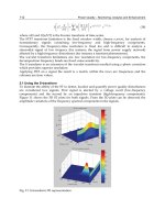
Figure 9.8a shows a visible satellite image (from a
geostationary satellite) of an occluded storm system in
the eastern Pacific. Notice that all of the clouds in the
photo appear white. However, in the infrared photo-
graph (Fig. 9.8b), taken on the same day (and just about
the same time), the clouds appear to have many shades
of gray. In the visible photograph, the clouds covering
part of Oregon and northern California appear rela-
tively thin compared to the thicker, bright clouds to the
west. Furthermore, these thin clouds must be high
because they also appear bright in the infrared picture.

Along the elongated band of clouds associated with
the occluded front, the clouds appear white and bright
in both pictures, indicating a zone of thick, heavy
clouds. Behind the front, the forecaster knows that the
lumpy clouds are probably cumulus because they
appear gray in the infrared photo, suggesting that their
tops are low and relatively warm.
When temperature differences are small, it is diffi-
cult to directly identify significant cloud and surface fea-
tures on an infrared picture. Some way must be found
to increase the contrast between features and their back-
grounds. This can be done by a process called computer
Weather Forecasting Methods and Tools 235
Earth surface
Cold
High cloud
Low cloud
Infrared energy
Infrared energy
Satellite
Appears
white
Infrared picture
Earth surface
Low cloud
Warm
Appears
gray
FIGURE 9.7
Generally, the lower the cloud, the warmer its top. Warm

objects emit more infrared energy than do cold objects. Thus,
an infrared satellite picture can distinguish warm, low (gray)
clouds from cold, high (white) clouds.
enhancement. Certain temperature ranges in the infra-
red photograph are assigned specific shades of gray—
grading from black to white. Figure 9.9 is an infrared-
enhanced picture for the same day and area as shown in
Fig. 9.8. Note the dark and light contouring in the pic-
ture. Clouds with cold tops, and those with tops near
freezing, are assigned the darkest gray color. Hence, the
dark gray areas embedded along the front represent the
region where the coldest and, therefore, highest and
thickest clouds are found. It is here where the stormiest
weather is probably occurring. Also notice that, near the
southern tip of the picture, the dark gray blotches sur-
rounded by areas of white are thunderstorms that have
developed over warm tropical waters. They show up
clearly as white, thick clouds in both the visible and
infrared photographs. By examining the movement of
these clouds on successive satellite photographs, the
forecaster can predict the arrival of clouds and storms,
and the passage of weather fronts.
The shades of gray on enhanced infrared photos
are often color-contoured to make specific features,
such as deep cloud layers and the freezing level, more
obvious. Usually, dark blue, red, or black is assigned
to clouds with the coldest (highest) tops. Figure 9.10
(p. 238) is a color-enhanced infrared satellite picture.
In regions where there are no clouds, it is difficult
to observe the movement of the air. To help with this

situation, the latest geostationary satellites are equipped
with water-vapor sensors that can profile the distribu-
tion of atmospheric water vapor in the middle and
upper troposphere (see Fig. 9.11, p. 238). In time-lapse
films, the swirling patterns of moisture clearly show wet
regions and dry regions, as well as middle tropospheric
swirling wind patterns and jet streams.
Up to this point, we have only looked at weather
forecasts made by high-speed computers using atmo-
spheric models. There are, however, other forecasting
methods, many of which have stood the test of time and
236 Chapter 9 Weather Forecasting
L
FIGURE 9.8
A visible image (a) and an infrared image (b) of the eastern Pacific taken on the same day at just about the same time.
(a) (b)
are based mainly on the experience of the forecaster.
Many of these techniques are of value, but often they
give more of a general overview of what the weather
should be like, rather than a specific forecast.
OTHER FORECASTING METHODS Probably the easiest
weather forecast to make is a persistence forecast,
which is simply a prediction that future weather will be
the same as present weather. If it is snowing today, a
persistence forecast would call for snow through
tomorrow. Such forecasts are most accurate for time
periods of several hours and become less and less accu-
rate after that.
Another method of forecasting is the steady-state,
or trend method. The principle involved here is that

surface weather systems tend to move in the same direc-
tion and at approximately the same speed as they have
been moving, providing no evidence exists to indicate
otherwise. Suppose, for example, that a cold front is
moving eastward at an average speed of 30 mi/hr and it
is 90 miles west of your home. Using the steady-state
method, we might extrapolate and predict that the front
should pass through your area in three hours.
In recent years, the trend method has been
employed in the making of forecasts from minutes for
up to a few hours. Such short-term forecasting has
come to be called nowcasting.
The analogue method is yet another form of
weather forecasting. Basically, this method relies on the
fact that existing features on a weather chart (or a series of
charts) may strongly resemble features that produced cer-
tain weather conditions sometime in the past. To the fore-
caster, the weather map “looks familiar,” and for this
reason the analogue method is often referred to as pattern
recognition. A forecaster might look at a prog and say, “I’ve
seen this weather situation before, and this happened.”
Prior weather events can then be utilized as a guide to the
future. The problem here is that, even though weather sit-
uations may appear similar, they are never exactly the
same. There are always sufficient differences in the vari-
ables to make applying this method a challenge.*
The analogue method can be used to predict a
number of weather elements, such as maximum tem-
perature. Suppose that in New York City the average
maximum temperature on a particular date for the past

30 years is 10°C (50°F). By statistically relating the max-
imum temperatures on this date to other weather ele-
ments—such as the wind, cloud cover, and humidity—a
relationship between these variables and maximum tem-
perature can be drawn. By comparing these relationships
with current weather information, the forecaster can
predict the maximum temperature for the day.
Predicting the weather by weather types employs
the analogue method. In general, weather patterns are
categorized into similar groups or “types,” using such
criteria as the position of the subtropical highs, the
upper-level flow, and the prevailing storm track. As an
Weather Forecasting Methods and Tools 237
FIGURE 9.9
An enhanced infrared image of the eastern Pacific taken on the
same day as the images shown in Fig. 9.8(a) and (b).
*Presently, however, statistical predictions are made routinely of weather
elements based on the past performance of computer models (the Model-
Output Statistics, or MOS). These, in effect, are statistically weighted ana-
logue forecast corrections to the computer model output.
Due to extremely limited availability of accurate weather
reports and forecasts, the average life expectancy for an
airmail pilot between 1918 and 1925 was about four
years.
238 Chapter 9 Weather Forecasting
FIGURE 9.10
A color-enhanced infrared satellite picture that shows a developing wave cyclone at 2
A.M. (EST)
on March 13, 1993. The darkest shades represent clouds with the coldest and highest tops. The
dark cloud band moving through Florida represents a line of severe thunderstorms. Notice that

the cloud pattern is in the shape of a comma.
FIGURE 9.11
Infrared water vapor image. The
darker areas represent dry air aloft;
the brighter the gray, the more
moist the air in the middle or
upper troposphere. Bright white
areas represent dense cirrus clouds
or the tops of thunderstorms. The
area in color represents the coldest
cloud tops. The swirl of moisture
off the West Coast represents a
well-developed mid-latitude
cyclonic storm.
example, when the Pacific high is weak or depressed
southward and the flow aloft is zonal (west-to-east),
surface storms tend to travel rapidly eastward across the
Pacific Ocean and into the United States without devel-
oping into deep systems. But when the Pacific high is to
the north of its normal position, and the upper airflow
is meridional (north-south), looping waves form in the
flow with surface lows usually developing into huge
storms. Since upper-level longwaves move slowly, usu-
ally remaining almost stationary for perhaps a few days
to a week or more, the particular surface weather at dif-
ferent positions around the wave is likely to persist for
some time. Figure 9.12 presents an example of weather
conditions most likely to prevail with a winter merid-
ional weather type.
Weather types can be used as an approach to long-

range (a month or more in advance) weather forecasting.
Typically, the upper-air circulation changes gradually
from zonal to meridional over 4 to 6 weeks. As this slow
change occurs in the upper air, the surface weather may
repeat itself at specific intervals. For instance, winter
cold fronts may sweep into New England every 4 days or
so, bringing showers and below-normal temperatures.
By projecting trends such as these, and assuming that
the atmosphere’s behavior will not change radically (an
assumption not always valid), extended weather forecasts
can be made. At best, these forecasts only show the
broad-scale weather features. They do not adequately
predict specific weather elements.
Currently, the Climate Prediction Center issues
extended forecasts of 6 to 10 days, as well as a 30-day out-
look for the coming month, and a 90-day seasonal
outlook. These are not forecasts in the strict sense, but
rather an overview of how average precipitation and tem-
perature patterns may compare with normal conditions.
To improve weather forecasts, meteorologists are
turning to a technique called ensemble forecasting.
This approach is based on running several forecast
models—or different versions (simulations) of a single
model—each beginning with slightly different weather
information to reflect the errors inherent in the mea-
surements. If, at the end of a specified time, the models
match each other fairly well, then the forecaster can
issue a prediction with a high degree of confidence. If
the models disagree, the forecaster, with little faith in
the computer model prediction, issues a forecast with

limited confidence, perhaps by giving a number ranging
from 0 (no confidence) to 5 (great confidence). In
essence, the less agreement among the models, the less pre-
dictable the weather. Consequently, it would not be wise
to make outdoor plans for Saturday when on Monday
the weekend forecast calls for “sunny and warm” with a
low degree of confidence.
A forecast based on the climatology (average
weather) of a particular region is known as a climato-
logical forecast. Anyone who has lived in Los Angeles
for a while knows that July and August are practically
rain-free. In fact, rainfall data for the summer months
taken over many years reveal that rainfall amounts of
more than a trace occur in Los Angeles about 1 day in
every 90, or only about 1 percent of the time. Therefore,
if we predict that it will not rain on some day next year
during July or August in Los Angeles, our chances are
nearly 99 percent that the forecast will be correct based
on past records. Since it is unlikely that this pattern will
significantly change in the near future, we can confi-
dently make the same forecast for the year 2020.
When the Weather Service issues a forecast calling
for rain, it is usually followed by a probability. For
example: “The chance of rain is 60 percent.” Does this
mean (a) that it will rain on 60 percent of the forecast
area or (b) that there is a 60 percent chance that it will
rain within the forecast area? Neither one! The expres-
sion means that there is a 60 percent chance that any
random place in the forecast area, such as your home,
will receive measurable rainfall.* Looking at the forecast

in another way, if the forecast for 10 days calls for a
Weather Forecasting Methods and Tools 239
Santa
Ana
Dry
Chinook
winds
Warm
Dr
y
Polar (arctic)
outbreaks
H
H
Stormy
Upper trough
U
p
p
e
r
-
a
i
r
fl
o
w
(
w

i
n
t
e
r
)
L
Pacific high
Upper ridge
H
FIGURE 9.12
Winter weather type showing upper airflow (heavy arrow), sur-
face position of Pacific high, and general weather conditions
that should prevail.
*The 60 percent chance of rain does not apply to a situation that involves rain
showers. In the case of showers, the percentage refers to the expected area
over which the showers will fall.
60 percent chance of rain, it should rain where you live
on 6 of those days. The verification of the forecast (as to
whether it actually rained or not) is usually made at the
Weather Service office, but remember that the com-
puter models make forecasts for a given area, not for an
individual location. When the National Weather Service
issues a forecast calling for a “slight chance of rain,”
what is the probability (percentage) that it will rain?
Table 9.1 provides this information.
An example of a probability forecast using clima-
tological data is given in Fig. 9.13. The map shows the
probability of a “White Christmas”—1 inch or more of
snow on the ground—across the United States. The

map is based on the average of 30 years of data and gives
the likelihood of snow in terms of a probability. For
instance, the chances are 90 percent (9 Christmases out
of 10) that portions of northern Minnesota, Michigan,
and Maine will experience a White Christmas. In
Chicago, it is 50 percent; and in Washington, D.C.,
about 20 percent. Many places in the far west and south
have probabilities less than 5 percent, but nowhere is the
probability exactly 0, for there is always some chance
(no matter how small) that a mantle of white will cover
the ground on Christmas Day.
In most locations throughout North America, the
weather is fair more often than rainy. Consequently,
there is a forecasting bias toward fair weather, which
means that, if you made a forecast of no-rain where you
live for each day of the year, your forecast would be cor-
rect more than 50 percent of the time. But did you show
any skill in making your correct forecast? What consti-
tutes skill, anyway? And how accurate are the forecasts
issued by the National Weather Service?
ACCURACY AND SKILL IN WEATHER FORECASTING In
spite of the complexity and ever-changing nature of
the atmosphere, forecasts made for between 12 and
24 hours are usually quite accurate. Those made for
between 1 and 3 days are fairly good. Beyond about
7 days, however, forecast accuracy falls off rapidly.
Although weather predictions made for up to 3 days are
by no means perfect, they are far better than simply flip-
ping a coin. But how accurate are they?
One problem with determining forecast accuracy

is deciding what constitutes a right or wrong forecast.
240 Chapter 9 Weather Forecasting
20 percent Slight chance of Widely scattered
precipitation showers
30 to 50 percent Chance of Scattered
precipitation showers
60 to 70 percent Precipitation likely Numerous
showers
≥ 80 percent Precipitation,* Showers*
rain, snow
*A forecast that calls for an 80 percent chance of rain in the after-
noon might read like this: “. . . cloudy today with rain this after-
noon. . . .” For an 80 percent chance of rain showers, the forecast
might read “. . . cloudy today with rain showers this afternoon. . . .”
Percent Forecast Wording Forecast Wording
Probability of for Steady for Showery
Precipitation Precipitation Precipitation
50
60 70
90
100
60
50
40
40
30
20
5
30
20

5
40
60
50
10
20
30
90
80
70
50
40
50
FIGURE 9.13
Probability of a “White Christmas”—one inch
or more of snow on the ground—based on a
30-year average. The probabilities do not include
the mountainous areas in the western United
States.
TABLE 9.1 Forecast Wording Used by the National Weather
Service to describe the percentage probability of measur-
able precipitation (0.01 inch or greater) for steady precip-
itation and for convective, showery precipitation.
Suppose tomorrow’s forecast calls for a minimum tem-
perature of 5°C. If the official minimum turns out to be
6°C, is the forecast incorrect? Is it as incorrect as one
10 degrees off? By the same token, what about a forecast
for snow over a large city, and the snow line cuts the city
in half with the southern portion receiving heavy
amounts and the northern portion none? Is the forecast

right or wrong? At present, there is no clear-cut answer
to the question of determining forecast accuracy.
How does forecast accuracy compare with forecast
skill? Suppose you are forecasting the daily summertime
weather in Los Angeles. It is not raining today and your
forecast for tomorrow calls for “no rain.” Suppose that
tomorrow it doesn’t rain. You made an accurate forecast,
but did you show any skill in so doing? In the previous
section, we saw that the chance of measurable rain in Los
Angeles on any summer day is very small indeed; chances
are good that day after day it will not rain. For a forecast
to show skill, it should be better than one based solely on
the current weather (persistence) or on the “normal”
weather (climatology) for a given region. Therefore, dur-
ing the summer in Los Angeles, a forecaster will have
many accurate forecasts calling for “no measurable rain,”
but will need skill to predict correctly on which summer
days it will rain.
Meteorological forecasts, then, show skill when
they are more accurate than a forecast utilizing only
persistence or climatology. Persistence forecasts are
Weather Forecasting Methods and Tools 241
As you watch the TV weathercaster,
you typically see a person describ-
ing and pointing to specific weather
information, such as satellite photos,
radar images, and weather maps,
as illustrated in Fig. 2. What you
may not know is that the weather-
caster is actually pointing to a blank

board (usually green or blue) on
which there is nothing (Fig. 3). This
process of electronically superimpos-
ing weather information in the TV
camera against a blank wall is
called color-separation overlay, or
chroma key.
The chroma key process works
because the studio camera is con-
structed to pick up all colors except
(in this case) blue. The various
maps, charts, satellite photos, and
other graphics are electronically
inserted from a computer into this
blue area of the color spectrum. The
person in the TV studio should not
wear blue clothes because such
clothing would not be picked up by
the camera—what you would see on
your home screen would be a head
and hands moving about the weather
graphics!
How, then, does a TV weather-
caster know where to point on the
blank wall? Positioned on each side
of the blue wall are TV monitors (look
carefully at Fig. 3) that weather-
casters watch so that they know
where to point.
TV WEATHERCASTERS—HOW DO THEY DO IT?

Focus on an Observation
FIGURE 2
On your home television, the weather forecaster appears to be point-
ing to weather information directly behind him.
FIGURE 3
In the studio, however, he is actually standing in front of a blank
board.
usually difficult to improve upon for a period of time of
several hours or less. Weather forecasts ranging from 12
hours to a few days generally show much more skill
than those of persistence. However, as the range of the
forecast period increases, the skill drops quickly. The 6–
to 10–day mean outlooks both show some skill (which
has been increasing over the last several decades) in pre-
dicting temperature and precipitation. However, the
accuracy of precipitation forecasts is less than that for
temperature. Presently, 7-day forecasts now show about
as much skill as 5-day forecasts did a decade ago.
Beyond 10 days, specific forecasts are only slightly better
than climatology.
Forecasting large-scale weather events several days
in advance (such as the blizzard of 1996 along the east-
ern seaboard of the United States) are far more accurate
than forecasting the precise evolution and movement of
small-scale, short-lived weather systems, such as torna-
does and severe thunderstorms. In fact, 3-day forecasts
of the development and movement of a major low-pres-
sure system show more skill today than 36-hour fore-
casts did 15 years ago.
Even though the precise location where a tornado

will form is presently beyond modern forecasting tech-
niques, the general area where the storm is likely to form
can often be predicted up to 3 days in advance. With
improved observing systems, such as Doppler radar and
advanced satellite imagery, the lead time of watches and
warnings for severe storms has increased. In fact, the
lead time* for tornado warnings has more than doubled
over the last decade.
In Chapter 7, we saw how a vast warming of the
equatorial tropical Pacific called El Niño can affect the
weather in different regions of the world. These inter-
actions, where a warmer tropical Pacific can influence
rainfall in California, are called teleconnections. These
types of interactions between widely separated regions
are identified through statistical correlations. For exam-
ple, over regions of North America, where temperature
and precipitation patterns tend to depart from normal
during El Niño and La Niña events, the Climate Predic-
tion Center can issue a forecast of an impending wetter
or drier season, months in advance. Forecasts using
teleconnections have shown promise. For example, as
the tropical equatorial Pacific became much warmer
than normal during the spring and early summer of
1997, forecasters predicted a wet rainfall season over
central and southern California. Although the heavy
rains didn’t begin until December, the weather during
the winter of 1997–1998 was wet and wild: Storm after
storm pounded the region, producing heavy rains, mud
slides, road closures, and millions of dollars in damages.
Brief Review

Up to this point, we have looked at the various methods
of weather forecasting. Before going on, here is a review
of some of the important ideas presented so far:
■ The forecasting of weather by high-speed computers
is known as numerical weather prediction. Mathemat-
ical models that describe how atmospheric tempera-
ture, pressure, and moisture will change with time are
programmed into the computer. The computer then
plots and draws surface and upper-air charts, and
produces a variety of forecast charts called progs.
■ After a number of days, flaws in the computer models
and small errors in the data greatly limit the accuracy
of weather forecasts.
■ A persistence forecast is a prediction that future
weather will be the same as the present weather,
whereas a climatological forecast is based on the cli-
matology of a particular region.
■ For a forecast to show skill, it must be better than a
persistence forecast or a climatological forecast.
■ Ensemble forecasting is a technique based on running
several forecast models (or different versions of a sin-
gle model), each beginning with slightly different
weather information to reflect errors in the measure-
ments. If the different versions agree fairly well, a
forecaster can place a high degree of confidence in the
forecast. A low degree of confidence means that the
models do not agree.
PREDICTING THE WEATHER FROM LOCAL SIGNS
Because the weather affects every aspect of our daily lives,
attempts to predict it accurately have been made for cen-

turies. One of the earliest attempts was undertaken by
Theophrastus, a pupil of Aristotle, who in 300
B.C. com-
piled all sorts of weather indicators in his Book of Signs. A
dominant influence in the field of weather forecasting for
2000 years, this work consists of ways to foretell the
weather by examining natural signs, such as the color and
shape of clouds, and the intensity at which a fly bites.
Some of these signs have validity and are a part of our
own weather folklore—“a halo around the moon por-
242 Chapter 9 Weather Forecasting
*Lead time is the interval of time between the issue of the warning and actual
observance of the tornado.
tends rain” is one of these. Today, we realize that the halo
is caused by the bending of light as it passes through ice
crystals and that ice crystal–type clouds (cirrostratus) are
often the forerunners of an approaching storm.
Weather predictions can be made by observing the
sky and using a little weather wisdom. If you keep your
eyes open and your senses keenly tuned to your envi-
ronment, you should, with a little practice, be able to
make fairly good short-range local weather forecasts by
interpreting the messages written in the weather ele-
ments. Table 9.2 is designed to help you with this
endeavor.
Weather Forecasting Methods and Tools 243
Surface winds from the S or Possible cool front and thunderstorms Possible showers; possibly turning
from the SW; clouds building approaching from the west cooler; windy
to the west; warm (hot) and
humid

Surface winds from the E or Possible approach of a warm front Possibility of precipitation within
from the SE, cool or cold; 12–24 hours; windy (rain with
high clouds thickening and possible thunderstorms during the
lowering; halo around the summer; snow changing to sleet or
sun or moon rain in winter)
Winter night
(a) If clear, relatively calm (a) Rapid radiational cooling will occur (a) A very cold night
with low humidity (low dew-
point temperature)
(b) If clear, relatively calm (b) Rapid radiational cooling will occur (b) A very cold night with
with low humidity and snow minimum temperatures lower
covering the ground than in (a)
(c) If cloudy, relatively calm (c) Clouds will absorb and radiate (c) Minimum temperature will
with low humidity infrared (IR) energy back to surface not be as low as in (a) or (b)
Summer night
(a) Clear, hot, humid (high (a) Strong absorption and emission (a) High minimum temperatures
dew points) of IR energy back to surface by water
vapor
(b) Clear and relatively dry (b) More rapid radiational cooling (b) Lower minimum temperatures
If surface winds are from the A surface high-pressure area may be Increasing clouds, warmer with
N and they become NE, then moving to your E, and a surface low- the possibility of precipitation
E, then SE (veering winds) pressure area may be approaching within 24 hours
from the W
If surface winds are from the A surface low-pressure area is moving Clearing and colder (cooler in
NE and they become N, then to your E, and a surface high-pressure summer)
NW (backing winds) area may be approaching from the W
Scattered cumulus clouds Atmosphere is relatively unstable Possible showers or thunder-
that show extensive vertical storms by afternoon with gusty
growth by mid morning winds
Afternoon cumulus clouds Stable layer above clouds (region Continued partly cloudy with no

with flat bases, and tops at dominated by high pressure) precipitation; probably clearing
just about the same level by nightfall
TABLE 9.2 Forecast at a Glance—Forecasting the Weather from Local Weather Signs.
Listed below are a few forecasting rules that may be applied when making a short-range local weather forecast.
Observation Indication Local Weather Forecast
Weather Forecasting
Using Surface Charts
We are now in a position to forecast the weather, utiliz-
ing more sophisticated techniques. Suppose, for exam-
ple, that we wish to make a short-range weather predic-
tion and the only information available is a surface
weather map. Can we make a forecast from such a
chart? Most definitely. And our chances of that forecast
being correct improve markedly if we have maps avail-
able from several days back. We can use these past maps
to locate the previous position of surface features and
predict their movement.
A simplified surface weather map is shown in Fig.
9.14. The map portrays early winter weather conditions
on Tuesday morning at 6:00
A.M. A single isobar is drawn
around the pressure centers to show their positions
without cluttering the map. Note that an open wave
cyclone is developing over the Central Plains with show-
ers forming along a cold front and light rain and snow
ahead of a warm front. The dashed lines on the map rep-
resent the position of the weather systems six hours ago.
Our first question is: How will these systems move?
DETERMINING THE MOVEMENT OF WEATHER SYSTEMS
There are several methods we can use in forecasting the

movement of surface pressure systems and fronts. The
following are a few of these forecasting rules of thumb:
1. For short-time intervals, storms and fronts tend to
move in the same direction and at approximately the
same speed as they did during the previous six hours
(providing, of course, there is no evidence to indicate
otherwise).
2. Lows tend to move in a direction that parallels the
isobars in the warm air ahead of the cold front.
3. Lows tend to move toward the region of greatest sur-
face pressure drop, whereas highs tend to move
toward the region of greatest surface pressure rise.
244 Chapter 9 Weather Forecasting
Groundhog Day, February 2, derives from certain
religious ceremonies performed before the birth of
Christ. Somehow, this date came to be considered the
midpoint of winter, and people, in an attempt to forecast
what the remaining half would be like, placed the
burden of weather prognosticator on the backs (or
rather, the shadows) of animals such as the groundhog.
•
SIMPLIFIED KEY
15
22
Wind direction (N)
–5
–9
10
0
12

–1
18
12
–10
–13
1034
–3
–5
14
3
18
8
21
16
31
26
1028
64
55
29
24
28
25
24
18
19
11
23
18
32

31
44
43
47
44
17
10
59
52
51
45
48
45
18
12
44
38
=•
38
18
10
21
13
–15
–18
38
36
44
39
17

14
1008
22
14
38
29
58
42
24
15
11
2
H
H
L
0 250 500 mi
0 400 800
km
Cold front
Warm front
Stationary front
Occluded front
Light snow
Light rain
Sleet
Windspeed (10 knots)
Air temperature 22°F
Dew point 15°F
29
FIGURE 9.14

Surface weather map for 6:00 A.M. Tuesday. Dashed lines indicate positions of weather
features six hours ago. Areas shaded green are receiving precipitation.
4. Surface pressure systems tend to move in the same
direction as the wind at 5500 m (18,000 ft)—the 500-
mb level. The speed at which surface systems move is
about half the speed of the winds at this level.
When the surface map (Fig. 9.14) is examined
carefully and when rules of thumb 1 and 2 are applied,
it appears that—based on present trends—the storm
center over the Central Plains should move northeast.
When we observe the 500-mb upper-air chart (Fig.
9.15), it too suggests that the surface low should move
northeast at a speed of about 25 knots.
A FORECAST FOR SIX CITIES We are now in a position
to make a weather forecast for six cities. To do this, we
will project the pressure systems, fronts, and current
weather into the future by assuming steady-state condi-
tions. Figure 9.16 gives the 12- and 24-hour projected
positions of these features.
A word of caution before we make our forecasts.
We are assuming that the pressure systems and fronts
are moving at a constant rate, which may or may not
occur. Storm systems, for example, tend to accelerate
until they occlude, after which their rate of movement
slows. Furthermore, the direction of moving systems
may change due to “blocking” highs and lows that exist
in their path or because of shifting upper-level wind
patterns. We will assume a constant rate of movement
and forecast accordingly, always keeping in mind that
the longer our forecasts extend into the future, the more

susceptible they are to error.
Using Fig. 9.16 to follow the storm center eastward,
we can make a basic forecast. The cold front moving
into north Texas on Tuesday morning is projected to
pass Dallas by that evening, so a forecast for the Dallas
area would be “warm with showers, then turning
colder.” But we can do much better than this. Knowing
the weather conditions that accompany advancing pres-
sure areas and fronts, we can make more detailed
weather forecasts that will take into account changes in
temperature, pressure, humidity, cloud cover, precipita-
tion, and winds. Our forecast will include the 24-hour
period from Tuesday morning to Wednesday morning
for the cities of Augusta, Georgia; Washington, D.C.;
Chicago, Illinois; Memphis, Tennessee; Dallas, Texas;
and Denver, Colorado. We will begin with Augusta.
Weather Forecasting Using Surface Charts 245
Miles
(statute)
per hour
Knots
Calm
Calm
1–2
3–8
9–14
15–20
21–25
26–31
32–37

38–43
44–49
50–54
55–60
61–66
67–71
72–77
78–83
84–89
119–123
1–2
3–7
8–12
13–17
18–22
23–27
28–32
33–37
38–42
43–47
48–52
53–57
58–62
63–67
68–72
73–77
103–107
L
L
5460

5520
5580
5640
5700
5760
FIGURE 9.15
A 500-mb chart for 6:00 A.M. Tuesday, showing wind flow. The light red L represents the
position of the surface low. The winds aloft tend to steer surface pressure systems along and,
therefore, indicate that the surface low should move northeastward at about half the speed of
the winds at this level, or 25 knots. Solid lines are contours in meters above sea level.
Weather Forecast for Augusta, Georgia On Tuesday
morning, continental polar air associated with a high
pressure center brought freezing temperatures and fair
weather to the Augusta area (see Fig. 9.14). Clear skies,
light winds, and low humidities allowed rapid night-
time cooling so that, by morning, temperatures were in
the low thirties. Now look closely at Fig. 9.16 and
observe that the anticyclone is moving slowly eastward.
Southerly winds on the western side of this system will
bring warmer and more moist air to the region. There-
fore, afternoon temperatures will be warmer than those
of the day before. As the warm front approaches from
the west, clouds will increase, appearing first as cirrus,
then thickening and lowering into the normal sequence
of warm-front clouds. Barometric pressure should fall.
Clouds and high humidity should keep minimum tem-
peratures well above freezing on Tuesday night. Note
that the projected area of precipitation (green-shaded
region) does not quite reach Augusta. With all of this in
mind, our forecast might sound something like this:

Clear and cold this morning with moderating tempera-
tures by afternoon. Increasing high clouds with skies
becoming overcast by evening. Cloudy and not nearly as
cold tonight and tomorrow morning. Winds will be
light and out of the south or southeast. Barometric pres-
sure will fall slowly.
Wednesday morning we discover that the weather
in Augusta is foggy with temperatures in the upper 40s
(°F). But fog was not in the forecast. What went wrong?
We forgot to consider that the ground was still cold
from the recent cold snap. The warm, moist air moving
over the cold surface was chilled below its dew point,
resulting in fog. Above the fog were the low clouds
we predicted. The minimum temperatures remained
higher than anticipated because of the release of latent
heat during fog formation and the absorption of
infrared energy by the fog droplets. Not bad for a start.
Now we will forecast the weather for Washington, D.C.
Rain or Snow for Washington, D.C.? Look at Fig. 9.16
and observe that the storm center is slowly approaching
Washington, D.C., from the west. Hence, the clear
weather, light southwesterly winds, and low temperatures
on Tuesday morning (Fig. 9.16) will gradually give way to
increasing cloudiness, winds shifting to the southeast,
and slightly higher temperatures. By Wednesday morn-
ing, the projected band of precipitation will be over the
city. Will it be in the form of rain or snow? Without a ver-
tical profile of temperature (a sounding), this question is
difficult to answer. We can see in Fig. 9.16, however, that
cities south of Washington, D.C.’s latitude are receiving

snow. So a reasonable forecast would call for snow, possi-
bly changing to rain as warm air moves in aloft in
advance of the approaching fronts. A 24-hour forecast for
Washington, D.C., might sound like this:
Increasing clouds today and continued cold. Snow
beginning by early Wednesday morning, possibly
246 Chapter 9 Weather Forecasting
•
Washington
24 Hour
6
:
0
0
A
.
M
.
H
H
L
•
•
•
•
•
Denver
12 Hour
Dallas
Chicago

12 Hour
Augusta
24 Hour
12
Hour
24
Hour
T
u
e
s
d
a
y
6
:
0
0
A
.
M
.
T
uesd
ay
6:
00
P
.M.
W

e
d
n
e
s
d
a
y
T
uesda
y
6:00
A
.M.
T
uesda
y
6:0
0
P
.M
.
W
ed
ne
sd
a
y
6
:00

A.M
.
Memphis
FIGURE 9.16
Projected 12- and 24-hour movement of
fronts, pressure systems, and precipitation
(shaded green area) from 6:00 A.M.
Tuesday until 6:00
A.M. Wednesday.
changing to rain. Winds will be out of the southeast.
Pressures will fall.
Wednesday morning a friend in Washington, D.C.,
calls to tell us that the sleet began to fall but has since
changed to rain. Sleet? Another fractured forecast! Well,
almost. What we forgot to account for this time was the
intensification of the storm. As the storm moved east-
ward, it deepened; central pressure lowered, pressure gra-
dients tightened, and southeasterly winds blew stronger
than anticipated. As air moved inland off the warmer
Atlantic, it rode up and over the colder surface air. Snow
falling into this warm layer at least partially melted; it
then refroze as it entered the colder air near ground level.
The influx of warmer air from the ocean slowly raised the
surface temperatures, and the sleet soon became rain.
Although we did not see this possibility when we made
our forecast, a forecaster more familiar with local sur-
roundings would have. Let’s move on to Chicago.
Big Snowstorm for Chicago From Figs. 9.14 and 9.16,
it appears that Chicago is in for a major snowstorm.
Overrunning of warm air has produced a wide area of

snow which, from all indications, is heading directly for
the Chicago area. Since cold air north of the low’s center
will be over Chicago, precipitation reaching the ground
should be frozen. On Tuesday morning the leading edge
of precipitation is less than six hours away from
Chicago. Based on the projected path of the storm, light
snow should begin to fall around noon.
By evening, as the storm intensifies, snowfall
should become heavy. It should taper off and finally end
around midnight as the storm moves on east. If it snows
for a total of twelve hours—six hours as light snow
(around one inch every three hours) and six hours as
heavy snow (around one inch per hour)—then the total
expected accumulation will be between six and ten
inches. As the low moves eastward, passing south of
Chicago, winds on Tuesday will gradually shift from
southeasterly to easterly, then northeasterly by evening.
Since the system is intensifying, it should produce
strong winds that will swirl the snow into huge drifts,
which may bring traffic to a crawl.
The winds will continue to shift to the north and
finally become northwesterly by Wednesday morning.
By then the storm center will probably be far enough
east so that skies should begin to clear. Cold air moving
in from the northwest behind the storm will cause tem-
peratures to drop further. Barometer readings during the
storm will fall as the low’s center approaches and reach a
low value sometime Tuesday night, after which they will
begin to rise. A weather forecast for Chicago might be:
Cloudy and cold with light snow beginning by noon,

becoming heavy by evening and ending by Wednesday
morning. Total accumulations will range between six
and ten inches. Winds will be strong and gusty out of
the east or northeast today, becoming northerly tonight
and northwesterly by Wednesday morning. Barometric
pressure will fall sharply today and rise tomorrow.
A call Wednesday morning to a friend in Chicago
reveals that our forecast was correct except that the total
snow accumulation so far is 13 inches. We were off in
our forecast because the storm system slowed as it
became occluded. We did not consider this because we
moved the system by the steady-state method. At this
time of year (early winter), Lake Michigan is not quite
frozen over and the added moisture picked up from the
lake by the strong easterly winds also helped to produce
a heavier-than-predicted snowfall. Again, a knowledge
of the local surroundings would have helped make a
more accurate forecast. The weather about 500 miles
south of Chicago should be much different from this.
Mixed Bag of Weather for Memphis Observe in Fig.
9.16 that, within twenty-four hours, both a warm and a
cold front should move past Memphis. The light rain that
began Tuesday morning should saturate the cool air, cre-
ating a blanket of low clouds and fog by midday. The
warm front, as it moves through sometime Tuesday after-
noon, should cause temperatures to rise slightly as winds
shift to the south or southwest. At night, clear to partly
cloudy skies should allow the ground and air above to
cool, offsetting any tendency for a rapid rise in tempera-
ture. Falling pressures should level off in the warm air,

then fall once again as the cold front approaches. Accord-
ing to the projection in Fig. 9.16, the cold front should
arrive sometime before midnight on Tuesday, bringing
with it gusty northwesterly winds, showers, the possibil-
ity of thunderstorms, rising pressures, and colder air.
Taking all of this into account, our weather forecast for
Memphis will be:
Cloudy and cool with light rain, low clouds, and fog
early today, becoming partly cloudy and warmer by late
this afternoon. Clouds increasing with possible showers
and thunderstorms later tonight or early Wednesday
morning and turning colder. Winds southeasterly this
morning, becoming southerly or southwesterly this
evening and shifting to northwesterly by Wednesday
morning. Pressures falling this morning, leveling off this
evening, then falling again tonight and rising by
Wednesday morning.
Weather Forecasting Using Surface Charts 247
A friend who lives near Memphis calls Wednesday
to inform us that our forecast was correct except that
the thunderstorms did not materialize and that Tuesday
night dense fog formed in low-lying valleys, but by
Wednesday morning it had dissipated. Apparently, in
the warm air, winds were not strong enough to mix the
cold, moist air that had settled in the valleys with the
warm air above. It’s on to Dallas.
Cold Wave for Dallas From Fig. 9.16, it appears that
our weather forecast for Dallas should be straightfor-
ward, since a cold front is expected to pass the area
around noon. Weather along the front is showery with a

few thunderstorms developing; behind the front the air
is clear but cold. By Wednesday morning it looks as if the
cold front will be far to the east and south of Dallas and
an anticyclone will be centered over Colorado. North or
northwesterly winds on the east side of the high will
bring cold continental polar air into Texas, dropping
temperatures as much as 40°F within a 24-hour period.
With minimum temperatures well below freezing, Dallas
will be in the grip of a cold wave. Our weather forecast
should therefore sound something like this:
Increasing cloudiness and mild this morning with the
possibility of showers and thunderstorms this after-
noon. Clearing and turning much colder tonight and
tomorrow. Winds will be southwesterly today, becoming
gusty north or northwesterly this afternoon and tonight.
Pressures falling this morning, then rising later today.
How did our forecast turn out? A quick call to Dal-
las on Wednesday morning reveals that the weather
there is cold but not as cold as expected, and the sky is
overcast. Cloudy weather? How can this be?
The cold front moved through on schedule Tues-
day afternoon, bringing showers, gusty winds, and cold
weather with it. Moving southward, the front gradually
slowed and became stationary along a line stretching
from the Gulf of Mexico westward through southern
Texas and northern Mexico. (From the surface map
alone, we had no way of knowing this would happen.)
Along the stationary front a wave formed. This wave
caused warm, moist Gulf air to slide northward up and
over the cold surface air. Clouds formed, minimum

temperatures did not go as low as expected, and we are
left with a fractured forecast. Let’s try Denver.
Clear but Cold for Denver In Fig. 9.16, we can see
that, based on our projections, the cold anticyclone will
be almost directly over Denver by Wednesday morning.
Sinking air aloft should keep the sky relatively free of
clouds. Weak pressure gradients will produce only weak
winds and this, coupled with dry air, will allow for
intense radiational cooling. Minimum temperatures
will probably drop to well below 0°F. Our forecast
should therefore read:
Clear and cold through tomorrow. Northerly winds
today becoming light and variable by tonight. Low tem-
peratures tomorrow morning will be below zero. Baro-
metric pressure will continue to rise.
Almost reluctantly Wednesday morning, we in-
quire about the weather conditions at Denver. “Clear
and very cold” is the reply. A successful forecast at last!
We are told, however, that the minimum temperature
did not go below zero; in fact, 13°F was as cold as it got.
A downslope wind coming off the mountains to the
west of Denver kept the air mixed and the minimum
temperature higher than expected. Again, a forecaster
familiar with the local topography of the Denver area
would have foreseen the conditions that lead to such
downslope winds and would have taken this into
account when making the forecast.
A complete picture of the surface weather systems
for 6:00
A.M. Wednesday morning is given in Fig. 9.17.

By comparing this chart with Fig. 9.16, we can summa-
rize why our forecasts did not turn out exactly as we
had predicted. For one thing, the storm center over the
Central Plains moved slower than expected. This slow
movement allowed a southeasterly flow of mild Atlan-
tic air to overrun cooler surface air ahead of the storm
while, behind the low, cities remained in the snow area
for a longer time. The weak wave that developed along
the trailing cold front brought cloudiness and pre-
cipitation to Texas and prevented the really cold air
from penetrating deep into the south. Further west, the
high originally over Montana moved more southerly
than southeasterly, which set up a pressure gradient
that brought westerly downslope winds to eastern
Colorado.
In summary, the forecasting techniques discussed
in this section are those you can use when making a
short-range weather forecast. Keep in mind, however,
that this chapter was not intended to make you an
expert weather forecaster, nor was it designed to show
you all the methods of weather prediction. It is hoped
that you now have a better understanding of some of
the problems confronting anyone who attempts to pre-
dict the behavior of this churning mass of air we call our
atmosphere.
248 Chapter 9 Weather Forecasting
Summary
Forecasting tomorrow’s weather entails a variety of
techniques and methods. Persistence and steady-state
forecasts are useful when making a short-range (0–6

hour) prediction. For a longer-range forecast, the cur-
rent analysis, satellite data, weather typing, intuition,
and experience, along with guidance from the many
computer progs supplied by the National Weather Ser-
vice, all go into making a prediction.
Different computer progs are based upon different
atmospheric models that describe the state of the atmos-
phere and how it will change with time. Currently, flaws
in the models—as well as tiny errors (uncertainties) in
the data—generally amplify as the computer tries to pro-
ject weather farther and farther into the future. At pre-
sent, computer progs are better at forecasting the position
of mid-latitude highs and lows and their development
than local showers and thunderstorms.
Satellites aid the forecaster by providing a bird’s-eye
view of clouds and storms. Polar-orbiting satellites obtain
data covering the earth from pole to pole, whereas geo-
stationary satellites situated above the equator supply the
forecaster with dynamic photographs of cloud and storm
development and movement. To show where the highest
and thickest clouds are located in a particular storm,
infrared pictures are often enhanced by computer.
In the latter part of this chapter, we learned how
people, by observing the weather around them, and by
watching the weather systems on surface weather maps,
can make fairly good short-range weather predictions.
Most of the forecasting methods in this chapter
apply mainly to skill in predicting events associated with
large-scale weather systems, such as fronts and mid-
latitude cyclones. The next chapter on severe weather

deals with the formation and forecasting of smaller-
scale (mesoscale) systems, such as thunderstorms,
squall lines, and tornadoes.
Key Terms
The following terms are listed in the order they appear in
the text. Define each. Doing so will aid you in reviewing
the material covered in this chapter.
Key Terms 249
1
0
0
0
•
•
°
•
1008
10
0
4
22
Chicago
9
9
6
24
48
Augusta
48
38

37
Washington
L
L
1024
13
5 Denver
1
0
2
0
10
16
10
1
2
1
0
1
6
10
0
8
Dallas
29
25
34
26
Memphis
••

••
••
•
H
•
FIGURE 9.17
Surface weather map for
6:00
A.M. Wednesday.
weather watch
weather warning
analysis
numerical weather
prediction
atmospheric models
prognostic chart (prog)
AW I PS
geostationary satellites
polar-orbiting satellites
persistence forecast
steady-state (trend)
forecast
nowcasting
Questions for Review
1. What is the function of the National Center for Envi-
ronmental Prediction?
2. How does a weather watch differ from a weather warn-
ing?
3. How does a prog differ from an analysis?
4. In what ways have high-speed computers assisted the

meteorologist in making weather forecasts?
5. How are computer-generated weather forecasts pre-
pared?
6. What are some of the problems associated with com-
puter model forecasts?
7. List some of the tools a weather forecaster uses when
making a forecast.
8. How do geostationary satellites differ from polar-
orbiting satellites?
9. (a) Explain how satellites aid in forecasting the
weather.
(b) Using infrared satellite information, how can a
forecaster distinguish high clouds from low
clouds?
(c) Why is it often necessary to enhance infrared
satellite images?
10. List four methods of forecasting the weather and give
an example for each one.
11. Suppose that where you live, the middle of January is
typically several degrees warmer than the rest of the
month. If you forecast this “January thaw” for the
middle of next January, what type of weather forecast
will you have made?
12. (a) Look out the window and make a persistence
forecast for tomorrow at this time.
(b) Did you use any skill in making this pre-
diction?
13. Do extended weather forecasts make specific predic-
tions of rain or snow? Explain.
14. Describe the technique of ensemble forecasting.

15. If today’s weather forecast calls for a “chance of snow,”
what is the percentage probability that it will snow
today? (Hint: See Table 9.1, p. 240.)
16. Do all accurate forecasts show skill on the part of the
forecaster? Explain.
17. List three methods that you would use to predict the
movement of a surface mid-latitude cyclonic storm.
Questions for Thought
and Exploration
1. What types of watches and warnings are most com-
monly issued for your area?
2. Since computer models have difficulty in adequately
considering the effects of small-scale geographic fea-
tures on a weather map, why don’t numerical weather
forecasters simply reduce the grid spacing to, say, 1
kilometer on all models?
3. Suppose it’s warm and raining outside. A cold front
will pass your area in 3 hours. Behind the front, it is
cold and snowing. Make a persistence forecast for
your area 6 hours from now. Would you expect this
forecast to be correct? Explain. Now, make a forecast
for your area using the steady-state or trend method.
4. How is the development of ensemble forecasting
methods linked to improvements in computer tech-
nologies?
5. Why isn’t the steady-state method very accurate when
forecasting the weather more than a few hours into the
future? What considerations can be taken into account
to improve a steady-state forecast?
6. Go outside and observe the weather. Make a weather

forecast using the weather signs you observe. Explain
the rationale for your forecast.
7. Using the Weather Forecasting/Forecasting section of
the
Blue Skies CD-ROM, make a weather forecast for
a specific city for five consecutive days. Compare your
forecasts with those made by the National Weather
Service. Keep track of the meteorological considera-
tions that went into your forecast.
8. Use the Weather Forecasting/Forecasting section of
the
Blue Skies CD-ROM to show current weather
and forecasts for a few different locations with
markedly differing synoptic-scale influences. Discuss
some of the important factors a forecaster must con-
sider, and how these factors differ from place to place.
9. Use the Weather Analysis/Isopleths section of the
Blue
Skies CD-ROM
and try your hand at drawing
isopleths.
10. Television weather forecasts for Milwaukee,
Wisconsin ( />( />For five days, compare weather forecasts made by two
television stations in a major U.S. city. What were the
major differences in the forecasts? Which station was
more accurate?
11. Computer model forecasts (l
.umich.edu/wxnet/model/model.html): Look at 12-,
24-, 36- and 48-hour forecast maps from a numerical
250 Chapter 9 Weather Forecasting

analogue forecasting
method
weather type forecasting
ensemble forecasting
climatological forecast
probability forecast
teleconnections
weather prediction model. Can you observe the life
cycle of a mid-latitude cyclone in the forecasts? De-
scribe the major weather conditions that are affecting
the forecast area.
12. Satellite Water Vapor Images (c
.wisc.edu/data/g8/latest_g8wv.gif and http://www
.ssec.wisc.edu/data/g9/latest_g9wv.gif): Examine cur-
rent water-vapor patterns as measured by satellites.
How do high areas of water vapor appear in the image?
What do dry areas look like?
For additional readings, go to InfoTrac College
Edition, your online library, at:

Questions for Thought and Exploration 251

What Are Thunderstorms?
Ordinary (Air-Mass) Thunderstorms
Severe Thunderstorms
The Gust Front and Microburst
Supercell and Squall-Line
Thunderstorms
Severe Thunderstorms and
the Dryline

Mesoscale Convective Complexes
Floods and Flash Floods
Focus on a Special Topic:
The Terrifying Flash Flood
in the Big Thompson Canyon
Distribution of Thunderstorms
Lightning and Thunder
Electrification of Clouds
The Lightning Stroke
Lightning Detection and Suppression
Focus on an Observation:
Don’t Sit Under the Apple Tree
To rn a d o e s
Tornado Occurrence
Tornado Winds
Tornado Formation
Observing Tornadoes
Focus on an Observation:
Thunderstorm Rotation
Severe Weather and Doppler Radar
Waterspouts
Summary
Key Terms
Questions for Review
Questions for Thought and Exploration
Contents
W
ednesday, March 18, 1925, was a day that began
uneventfully, but within hours turned into a day that
changed the lives of thousands of people and made meteorological

history. Shortly after 1:00
P.M., the sky turned a dark greenish-black
and the wind began whipping around the small town of Murphysboro,
Illinois. Arthur and Ella Flatt lived on the outskirts of town with their only
son, Art, who would be four years old in two weeks. Arthur was
working in the garage when he heard the roar of the wind and saw
the threatening dark clouds whirling overhead. Instantly concerned for
the safety of his family, he ran toward the house as the tornado began
its deadly pass over the area. With debris from the house flying in his
path and the deafening thunder of destruction all around him, Arthur
reached the front door. As he struggled in vain to get to his family,
whose screams he could hear inside, the porch and its massive support
pillars caved in on him. Inside the house, Ella had scooped up young
Art in her arms and was making a panicked dash down the front
hallway towards the door when the walls collapsed, knocking her to
the floor, with Art cradled beneath her. Within seconds, the rest of the
house fell down upon them. Both Arthur and Ella were killed instantly,
but Art was spared, nestled safely under his mother’s body.
As the dead and survivors were pulled from the devastation that
remained, the death toll mounted. Few families escaped the grief of lost
loved ones. The infamous tri-state tornado killed 234 people in
Murphysboro and leveled 40 percent of the town.
Thunderstorms and Tornadoes
253
T
he devastating tornado described in our opening
cut a mile-wide path for a distance of more than
200 miles through the states of Missouri, Illinois, and
Indiana. The tornado (which was most likely a series of
tornadoes) totally obliterated 4 towns, killed an esti-

mated 695 persons, and left over 2000 injured. Torna-
does such as these, as well as much smaller ones, are
associated with severe thunderstorms. Consequently, we
will first examine the different types of thunderstorms.
Later, we will focus on tornadoes, examining how and
where they form, and why they are so destructive.
What Are Thunderstorms?
It probably comes as no surprise that a thunderstorm is
merely a storm containing lightning and thunder. Some-
times a thunderstorm produces gusty surface winds with
heavy rain and hail. The storm itself may be a single
cumulonimbus cloud, or several thunderstorms may
form a cluster, or a line of thunderstorms may form that
in some cases may extend for hundreds of kilometers.
The birth of a thunderstorm occurs when warm,
humid air rises in a conditionally unstable environ-
ment.* The trigger needed to start air moving upward
may be the unequal heating of the surface, the effect of
terrain, or the lifting of warm air along a frontal zone.
Diverging upper-level winds, coupled with converging
surface winds and rising air, also provide a favorable
condition for thunderstorm development. Usually, sev-
eral of these mechanisms work together to generate
severe thunderstorms.
Scattered thunderstorms that form in summer are
often referred to as ordinary thunderstorms, formerly
air-mass thunderstorms, because they tend to develop in
warm, humid air masses away from weather fronts.
These storms are usually short-lived and rarely produce
strong winds or large hail. On the other hand, severe

thunderstorms may produce high winds, flash floods,
damaging hail, and even tornadoes. Let’s examine the
ordinary thunderstorms first.
Ordinary (Air-Mass) Thunderstorms
Extensive studies indicate that thunderstorms go through
a cycle of development from birth to maturity to decay.
The first stage is known as the cumulus stage. As humid
air rises, it cools and condenses into a single cumulus
cloud or a cluster of clouds (see Fig. 10.1). If you have
ever watched a thunderstorm develop, you may have
noticed that at first the cumulus clouds grow upward
only a short distance, then they dissipate. This sequence
happens because the cloud droplets evaporate as the drier
air surrounding the cloud mixes with it. However, after
the water drops evaporate, the air is more moist than
before. So, the rising air is now able to condense at suc-
cessively higher levels, and the cumulus cloud grows
taller, often appearing as a rising dome or tower.
As the cloud builds, the transformation of water
vapor into liquid or solid cloud particles releases large
quantities of latent heat. This keeps the air inside the
cloud warmer than the air surrounding it. The cloud
continues to grow in the unstable atmosphere as long
as it is constantly fed by rising air from below. In this
manner, a cumulus cloud may show extensive vertical
development in just a few minutes. During the cumulus
stage, there is insufficient time for precipitation to form,
and the updrafts keep water droplets and ice crystals
suspended within the cloud. Also, there is no lightning
or thunder during this stage.

As the cloud builds well above the freezing level, the
cloud particles grow larger. They also become heavier.
Eventually, the rising air is no longer able to keep them
suspended, and they begin to fall. While this phenome-
non is taking place, drier air from around the cloud is
being drawn into it in a process called entrainment. The
entrainment of drier air causes some of the raindrops to
evaporate, which chills the air. The air, now being colder
and heavier than the air around it, begins to descend as a
downdraft. The downdraft may be enhanced as falling
precipitation drags some of the air along with it.
254 Chapter 10 Thunderstorms and Tornadoes
*Thunderstorms may form when a cold “pool” of air moves over a region
where the surface air temperature is no more than 10°C (50°F). This situa-
tion often occurs during the winter along the west coast of North America.
Additionally, thunderstorms occasionally form in wintertime snowstorms. In
both of these cases, the air aloft is considerably colder than the surface air,
which generates instability.
Dissipating
32°F
0°C
Cumulus
Mature
FIGURE 10.1
Simplified model depicting the life cycle of an ordinary
thunderstorm that is nearly stationary. (Arrows show vertical air
currents. Dashed line represents freezing level, 0°C isotherm.)
The appearance of the downdraft marks the begin-
ning of the mature thunderstorm. The downdraft and
updraft within the mature thunderstorm constitute a

cell.* In most storms, there are several cells, each of
which may last for an hour or so.
During its mature stage, the thunderstorm is most
intense. The top of the cloud, having reached a stable
region of the atmosphere (which may be the strato-
sphere), begins to take on the familiar anvil shape, as
strong upper-level winds spread the cloud’s ice crystals
horizontally (see Fig. 10.2). The cloud itself may extend
upward to an altitude of over 12 km (40,000 ft) and be
several kilometers in diameter near its base. Updrafts and
downdrafts reach their greatest strength in the middle of
the cloud, creating severe turbulence. In some storms, the
updrafts may intrude above the cloud top into the stable
atmosphere, a condition known as overshooting. Light-
ning and thunder are also present in the mature stage.
Heavy rain (and occasionally small hail) falls from the
cloud. There is often a downrush of cold air with the
onset of precipitation at the surface that may be felt as a
strong wind gust. The rainfall, however, may or may not
reach the surface, depending on the relative humidity
beneath the storm. In the dry air of the desert Southwest,
for example, a mature thunderstorm may look ominous
and contain all of the ingredients of any other storm,
except that the raindrops evaporate before reaching the
ground. However, intense downdrafts from the storm
may reach the surface, producing strong, gusty winds.
After the storm enters the mature stage, it begins
to dissipate in about 15 to 30 minutes. The dissipating
stage occurs when the updrafts weaken and downdrafts
tend to dominate throughout much of the cloud. De-

prived of the rich supply of warm humid air, cloud
droplets no longer form. Light precipitation now falls
from the cloud, accompanied by only weak downdrafts.
As the storm dies, the lower-level cloud particles evapo-
rate rapidly (see Fig. 10.3), sometimes leaving only a cir-
rus anvil as the reminder of the once mighty presence.
A single ordinary thunderstorm may go through its
three stages in an hour or less. The reason it does not last
very long is that the storm’s downdraft may cut off the
storm’s fuel supply by destroying the humid updrafts.
Not only do thunderstorms produce summer rain-
fall for a large portion of the United States but they also
bring with them momentary cooling after an oppres-
sively hot day. The cooling comes during the mature
stage, as the downdraft reaches the surface in the form
of a blast of welcome relief. Sometimes, the air temper-
ature may lower as much as 10°C (18°F) in just a few
minutes. Unfortunately, the cooling effect is short-lived,
as the downdraft diminishes or the thunderstorm
moves on. In fact, after the storm has ended, the air
temperature usually rises; and as the moisture from the
rainfall evaporates into the air, the humidity increases,
sometimes to a level where it actually feels more oppres-
sive after the storm than it did before.
Upon reaching the surface, the cold downdraft has
another effect. It may force warm, moist surface air
upward. This rising air then condenses and gradually
builds into a new thunderstorm. Thus, it is entirely pos-
sible for a series of thunderstorms to grow in a line, one
next to the other, each in a different stage of develop-

ment (see Fig. 10.4). Thunderstorms that form in this
manner are termed multicell storms. Most ordinary
Ordinary (Air-Mass) Thunderstorms 255
*In convection, the cell may be a single updraft or a single downdraft, or a
couplet of the two, which defines the mature stage of the thunderstorm.
FIGURE 10.2
An ordinary thunderstorm in
its mature stage. Note the
distinctive anvil top.
thunderstorms are multicell storms, as are most severe
thunderstorms.
As we saw earlier in this chapter, for a thunder-
storm to develop there must be rising, moist air in a
conditionally unstable atmosphere. The ingredient nec-
essary to start the air rising may be the unequal heating
of the surface, a frontal boundary, a mountain range, or
the leading edge of a sea breeze. Most of the thunder-
storms that form in this manner are not severe, and
their life cycle usually follows the pattern described for
ordinary thunderstorms.
Severe Thunderstorms
Severe thunderstorms are capable of producing large
hail, strong, gusty surface winds, flash floods, and tor-
nadoes.* Just as the ordinary thunderstorm, they form
as moist air is forced to rise into a conditionally unstable
atmosphere. But, severe thunderstorms also form in
areas with a strong vertical wind shear.
Strong winds aloft may cause the updrafts in a
severe thunderstorm to tilt in its mature stage, as de-
picted in Fig. 10.5. The storm is moving from left to

right and the upper-level winds cause the system to tilt
so that the updrafts move up and over the downdrafts.
This situation allows the updraft to remain strong for an
extended period of time. However, there are many
severe thunderstorms that do not have a tilted updraft.
In these storms, the updrafts may be so strong (some-
times up to 100 knots) that precipitation-size particles
256 Chapter 10 Thunderstorms and Tornadoes
FIGURE 10.3
A dissipating thunderstorm near Naples, Florida. Most of the cloud particles in the lower
half of the storm have evaporated.
On July 13, 1999, in Sattley, California, a strong down-
draft from a mature thunderstorm dropped the air
temperature from 97°F at 4:00
P.M. to a chilly 57°F one
hour later.
*The National Weather Service defines a severe thunderstorm as having 3⁄4-
inch hail and/or surface wind gusts of 50 knots (58 mi/hr).
do not have enough time to form. Apparently, this type
of thunderstorm becomes severe when a strong vertical
wind shear causes the storm to rotate. And, as we will
discuss later in this chapter, it is the rotational aspect of
thunderstorms that leads to the formation of tornadoes.
The updrafts in a severe thunderstorm may be so
strong that the cloud top is able to intrude well into the
stable stratosphere. In some cases, the top of the cloud
may extend to more than 18 km (60,000 ft) above the
surface. The violent updrafts keep hailstones suspended
in the cloud long enough for them to grow to consider-
able size. Once they are large enough, they either fall out

the bottom of the cloud with the downdraft or a strong
updraft may toss them out the side of the cloud, or even
from the base of the anvil. Aircraft have actually encoun-
tered hail in clear air several kilometers from a storm.
Also, downdrafts within the anvil may produce beautiful
mammatus clouds.
As some of the falling precipitation evaporates, it
cools the air and enhances the downdraft. The cool air
that reaches the ground may act like a wedge, forcing
warm, moist surface air up into the system (see Fig.
10.6). Thus, the downdraft may help to maintain the
updraft and vice versa, so that a severe thunderstorm
with this type of updraft and downdraft configuration
is able to maintain itself (for many hours in some cases).
THE GUST FRONT AND MICROBURST Look at Fig. 10.6
again and notice that the downdraft spreads laterally
after striking the ground. The boundary separating this
cold downdraft from the warm surface air is known as a
gust front. To an observer on the ground, the passage of
the gust front resembles that of a cold front. During its
passage, the wind shifts and becomes strong and gusty,
with speeds occasionally exceeding 55 knots; tempera-
tures drop sharply and, in the cold heavy air of the
Severe Thunderstorms 257
FIGURE 10.4
A multicell storm. This
storm is composed of a
series of cells in successive
stages of growth. The
thunderstorm in the

middle is in its mature
stage, with a well-defined
anvil. Heavy rain is falling
from its base. To the right
of this cell, a thunder-
storm is in its cumulus
stage. To the left, a well-
developed cumulus
congestus cloud is about
ready to become a mature
thunderstorm.
Rain
Hail
Mammatus
Wind
Tropopause
Overshooting top
Anvil
•
•
•
•
•
•
•
•
•
•
•
•

•
•
•
•
•
•
•
•
•
•
•
•
•
•
•
•
•
•
•
•
•
•
•
•
•
•
•
•
•
•

•
•
•
•
•
•
•
•
•
•
•
•
•
•
•
•
•
•
•
•
•
•
•
•
•
•
•
•
•
•

•
•
•
•
•
•
•
•
•
•
•
•
•
•
•
•
•
•
•
•
•
•
•
•
•
•
•
•
•
•

•
•
•
•
•
•
•
•
•
•
•
•
•
•
•
•
•
•
•
•
•
•
•
•
•
•
•
•
•
•

•
•
•
•
•
•
•
•
•
•
•
•
•
•
•
•
•
•
•
•
•
•
•
•
•
•
•
•
•
•

•
•
•
•
•
•
•
FIGURE 10.5
A simplified model
describing air motions
and other features
associated with a severe
thunderstorm that has a
tilted updraft. The severity
depends on the intensity
of the storm’s circulation
pattern.
downdraft, the surface pressure rises. Sometimes it may
jump several millibars, producing a small area of high
pressure called a mesohigh (meaning mesoscale high).
The cold air may linger close to the ground for several
hours, well after the thunderstorm activity has ceased.
Along the leading edge of the gust front, the air is
quite turbulent. Here, strong winds can pick up loose
dust and soil and lift them into a huge tumbling cloud—
the haboob that we described in Chapter 7. As warm,
moist air rises along the forward edge of the gust front,
a shelf cloud (also called an arcus cloud) may form, such
as the one shown in Fig. 10.7. These clouds are especially
prevalent when the atmosphere is very stable near the

base of the thunderstorm. Look back at Fig. 10.6 and
notice that the shelf cloud is attached to the base of the
thunderstorm. Occasionally, an elongated ominous-
looking cloud forms just behind the gust front. These
clouds, which appear to slowly spin about a horizontal
axis, are called roll clouds (see Fig. 10.8). Sometimes the
leading edge of the gust front forces warm, moist air
upward, producing new thunderstorms.
Beneath a severe thunderstorm, the downdraft
may become localized so that it hits the ground and
spreads horizontally in a radial burst of wind, much like
water pouring from a tap and striking the sink below.
Such downdrafts are called downbursts. A downburst
with winds extending only 4 kilometers or less is termed
a microburst. In spite of its small size, an intense micro-
burst can induce damaging winds as high as 146 knots.
(A larger downburst with winds extending more than
4 kilometers is termed a macroburst.) Figure 10.9 shows
the dust clouds generated from a microburst north of
Denver, Colorado. Since a microburst is an intense
downdraft, its leading edge can evolve into a gust front.
258 Chapter 10 Thunderstorms and Tornadoes
Rain area
Gust front
Cool air
Stable air
Warm
moist air
Shelf cloud
Drier air

Drier air
Downdraft
Updraft
FIGURE 10.6
The lower half of a severe squall-line-type thunderstorm and
some of the features associated with it.
FIGURE 10.7
A dramatic example of a shelf cloud (or arcus cloud) associated with a severe thunderstorm.
Microbursts are capable of blowing down trees and
inflicting heavy damage upon poorly built structures. In
fact, microbursts may be responsible for some damage
once attributed to tornadoes. Moreover, microbursts
and their accompanying wind shear (that is, rapid
changes in wind speed or wind direction) appear to be
responsible for several airline crashes. When an aircraft
flies through a microburst at a relatively low altitude,
say 300 m (1000 ft) above the ground, it first encounters
a headwind that generates extra lift. However, in a mat-
ter of seconds, the headwind is replaced by a tailwind
that causes a sudden loss of lift and a subsequent
decrease in the performance of the aircraft.
One accident attributed to a microburst occurred
north of Dallas–Fort Worth Regional Airport during
August, 1985. Just as the aircraft was making its final
approach, it encountered severe wind shear beneath a
small, but intense thunderstorm. The aircraft then
dropped to the ground and crashed, killing over 100
passengers.
To detect the hazardous wind shear associated with
microbursts, a new and improved ground-based wind-

shear detection system called LLWSAS (for Low-Level
Wind Shear Alert System) has been installed at several
airports. The system utilizes surface wind speed and
direction sensors to measure the presence of wind shear.
Severe Thunderstorms 259
FIGURE 10.8
A roll cloud forming behind a gust front. (Copyright Howard B. Bluestein.)
Unfortunately, LLWSAS can only detect a microburst
after it hits the ground and only where the instruments
are located. However, the installation of Doppler radars
throughout the United States is providing a better
system of detecting microbursts and other severe
weather phenomena.
Microbursts can be associated with severe thunder-
storms, producing strong, damaging winds. But studies
show that they can also occur with ordinary thunder-
storms, and with clouds that produce only isolated
showers—clouds that may or may not contain thunder
and lightning.
The strong downburst winds associated with a clus-
ter of severe thunderstorms can produce damaging
straight-line winds* that may exceed 90 knots. If the wind
damage extends for at least 400 km (250 mi) along the
storm’s path, the winds are called a derecho (day-ray-
cho), after the Spanish word for “straight ahead.” Most
derechoes are associated with severe thunderstorms that
extend outward in the shape of a bow echo on a radar
screen (see Fig. 10.10). Typically, derechoes form in the
early evening and last throughout the night. An especially
powerful derecho roared through New York State during

*Straight-line winds are thunderstorm-generated winds that are not associ-
ated with rotation.