- Trang chủ >>
- Khoa Học Tự Nhiên >>
- Vật lý
The Lecture Notes in Physics Part 5 ppsx
Bạn đang xem bản rút gọn của tài liệu. Xem và tải ngay bản đầy đủ của tài liệu tại đây (188.64 KB, 21 trang )
74 X. Carton
can be represented as a stack of homogeneous layers and that vortices are con-
fined in one layer, or in a few of these layers. A central property of these models
is conservation of potential vorticity in unforced, non-dissipative flows. Indeed,
potential vorticity conjugates many vortex properties (internal vorticity, relation
with planetary vorticity, and the vertical stretching of water columns) in a single
variable.
3.2.1 Primitive-Equation Model
The primitive equations are the Navier–Stokes equations on a rotating planet, for
an incompressible fluid, with Boussinesq and hydrostatic approximations. These
dynamical equations are complemented with an equation of state for the fluid and
with advection–diffusion equations for temperature and salinity (in the ocean). They
are usually written as
Du
Dt
− f v =
−1
ρ
0
∂
x
p + F
x
+ D
x
,
Dv
Dt
+ fu =
−1
ρ
0
∂
y
p + F
y
+ D
y
for the two horizontal momentum equations (ρ
0
being an average density),
∂
z
p =−ρg
for the hydrostatic balance,
ρ = ρ(T, S, p)
for the equation of state,
∂
x
u + ∂
y
v +∂
z
w = 0
for the incompressibility equation, and
DT
Dt
= κ
T
∇
2
T + F
T
DS
Dt
= κ
S
∇
2
S + F
S
for the temperature and salinity equations (T is temperature and S is salinity). The
Lagrangian advection is three-dimensional D/Dt = ∂
t
+ u∂
x
+ v∂
y
+ w∂
z
.The
3 Oceanic Vortices 75
Coriolis parameter is f = 2 sin(θ), where is the rotation rate of the Earth
and θ is latitude; g is gravity. F
x
, F
y
and D
x
, D
y
are the forcing and dissipative
terms in the horizontal momentum equations, and F
T
, F
S
are the source terms in
the thermodynamics/tracer equations. The thermal and salt diffusivities are κ
T
and
κ
S
, respectively.
This system is associated with a set of boundary conditions: mechanical, thermal,
and haline forcing at the sea surface, interaction with bottom topography, and pos-
sible lateral forcing via exchanges between ocean basins.
Primitive equations conserve potential vorticity in adiabatic, inviscid evolutions;
this potential vorticity has the form
= (ω + f k) ·
∇ρ
ρ
,
with ω = (−∂
z
v, ∂
z
u,∂
x
v −∂
y
u).
The primitive equations can be rendered non-dimensional. Non-dimensional num-
bers quantify the intensity of each physical effect:
- the Rossby number Ro = U/fL, where U is a horizontal velocity scale and L
a horizontal length scale characterizes the influence of planetary rotation on the
motion (this number is the ratio of inertial to Coriolis accelerations),
- the Burger number Bu = N
2
H
2
/ f
2
L
2
, where N
2
=−(g/ρ)∂
z
ρ is the Brunt–
Väisälä frequency and H is a vertical length scale, indicates the influence of
stratification on motion (it is the ratio of buoyancy to Coriolis terms),
- the Reynolds number Re = UL/ν, where ν is viscosity, is the ratio of lateral
friction to acceleration and it characterizes the influence of dissipation on motion,
- the Ekman number Ek = ν/fH
2
is the ratio of vertical dissipation to Coriolis
acceleration and characterizes the importance of frictional effects at the ocean
surface and bottom,
- the aspect ratio of motions, H/L, also indicates how efficiently planetary rotation
and ambient stratification have confined motions in the horizontal plane.
These non-dimensional numbers are used to derive the simplified equation sys-
tems (shallow-water and quasi-geostrophic models). In particular, for unforced, non-
dissipative motions, a small Rossby number (associated with small aspect ratio of
the motion) indicates that the Coriolis acceleration balances the horizontal pressure
gradient:
f v =
1
ρ
0
∂
x
p
fu=
−1
ρ
0
∂
y
p.
These equations are called the geostrophic balance. Using now the hydrostatic bal-
ance, and under the same conditions, we obtain the thermal wind relations
76 X. Carton
f ∂
z
u =
−g
ρ
0
∂
x
ρ,
f ∂
z
v =
g
ρ
0
∂
y
ρ,
which indicates that the vertical shear of horizontal velocity is then related to the
horizontal density gradients.
The primitive-equation model has been used for the study of vortex generation
by deep ocean jets or by coastal currents.
Along the continental shelf from the Florida Straits to Cape Hatteras, the Gulf
Stream is a frontal current and it can undergo frontal baroclinic instability, leading
to the formation of meanders and cyclones. With a primitive-equation model, Oey
[115] showed that the relative thickness of the upper ocean layer and the distance of
the front from the continental slope govern the frontal baroclinic instability. Chao
and Kao [26] evidenced successive barotropic and baroclinic instabilities on this
current and the formation of anticyclones. To analyze the formation of meanders
and rings in the Gulf Stream region east of Cape Hatteras, Spall and Robinson [147]
used a primitive-equation, open-ocean model, and they showed that bottom topog-
raphy plays an important role in the structure of the deep flow. Warm-core ring
formation results from differential horizontal advection of a developed meander,
while cold-core ring formation involves geostrophic and ageostrophic horizontal
advection, vertical advection, and baroclinic conversion.
With a primitive-equation model, Lutjeharms et al. [93] studied the formation of
shear edge eddies from the Agulhas Current along the Agulhas Bank. These eddies,
with a diameter of 50–100 km, are prevalent in the Agulhas Bank shelf bight as
observed, and their leakage may trigger the detachment of cyclones from the tip of
the Agulhas Bank. These cyclones have sometimes been observed to accompany the
detachment of Agulhas rings from the Agulhas Current.
More recently, the primitive-equation model was used for the study of ocean
surface turbulence, vertical motions and the coupling of physics with biology, via
submesoscale motions. Levy et al. [88] modeled jet instability at very high reso-
lution and showed that submesoscale physics reinforce the mesoscale eddy field.
Submesoscale structures (filaments) are associated with strong density and vorticity
gradients and are located between the eddies. They also induce large vertical veloc-
ities, which inject nutrients in the upper ocean layer. This study was complemented
by that of Lapeyre and Klein [84] who showed that elongated filaments are more
efficient than curved filaments at injecting nutrients vertically.
3.2.2 The Shallow-Water Model
3.2.2.1 Equations and Potential Vorticity Conservation
At eddy scale or even at the synoptic scale (a few hundred kilometers horizon-
tally), the ocean can be modeled as a stack of homogeneous layers in which the
3 Oceanic Vortices 77
motion is essentially horizontal (due to Coriolis force and stratification). In each
layer, horizontal homogeneity leads to vertically uniform horizontal velocities.
The shallow-water equations are obtained by integrating the horizontal momentum
and the incompressibility equations over each layer thickness. Here, we write the
shallow-water equations in polar coordinates for application to vortex dynamics (u
j
is radial velocity and v
j
is azimuthal velocity):
Du
j
Dt
− f v
j
=
−1
ρ
j
∂
r
p
j
+ F
rj
+ D
rj
Dv
j
Dt
+ fu
j
=
−1
rρ
j
∂
θ
p
j
+ F
θ j
+ D
θ j
Dh
j
Dt
+ h
j
∇ · u
j
=
Dh
j
Dt
+
h
j
r
(∂
r
(ru
j
) + ∂
θ
v
j
) = 0, (3.1)
with
D
Dt
= ∂
t
+ u
j
∂
r
+ (v
j
/r)∂
θ
.
Here p
j
, h
j
,ρ
j
, F
j
, and D
j
are pressure, local thickness, density, body force, and
viscous dissipation, respectively in layer j ( j varying from 1 at the surface to N
at the bottom); f = f
0
+ βy is the expansion of the spherical expression of f on
the tangential plane to Earth at latitude θ
0
. The local and instantaneous thickness is
h
j
= H
j
+η
j−1/2
−η
j+1/2
, where H
j
is the thickness of the layer at rest and η
j+1/2
is the interface elevation between layer j and layer j +1 due to motion. We choose
to impose a rigid lid on the ocean surface (η
1/2
= 0) and the bottom topography is
represented by η
N+1/2
= h
B
(x, y) (see Fig. 3.8). Finally, the hydrostatic balance is
written as p
j
= p
j−1
+ g(ρ
j
− ρ
j−1
)η
j−1/2
.
An essential property of these equations is layerwise potential vorticity conservation
in the absence of forcing and of dissipation (F
j
= D
j
= 0). By taking the curl of
the momentum equations, and by substituting the horizontal velocity divergence in
the continuity equation, Lagrangian conservation of layerwise potential vorticity
j
is obtained:
d
j
dt
= 0,
j
=
ζ
j
+ f
0
+ βy
h
j
, (3.2)
with ζ
j
= (1/r)[∂
r
(rv
j
) − ∂
θ
u
j
] the relative vorticity.
For vortex motion, it is more convenient to introduce the PV anomaly with respect
to the surrounding ocean at rest. For instance, in the case of f -plane dynamics
Q
j
=
j
−
0
j
=
ζ
j
+ f
0
h
j
−
f
0
H
j
=
1
h
j
ζ
j
− f
0
δη
j
H
j
,
78 X. Carton
z
H1
η3/2
H2
hB
η5/2
u1,v1,p1
ρ1
ρ2
u2,v2,p2
ηΝ−1/2
uN,vN,pN
ρΝ
surface
HN
bottom
f0
g
Fig. 3.8 Sketch of a N-layer ocean for the shallow-water model
where δη
j
= h
j
− H
j
is the vertical deviation of isopycnals across the vortex.
Obviously, the PV anomaly is then conserved. On the beta-plane, one usually does
not include planetary vorticity in the PV anomaly, which is then not conserved [108].
To evaluate the potential vorticity contents of each layer, we restore the forcing
and dissipation terms, so that
d
j
dt
=
1
h
j
1
r
∂
r
(r(F
θ j
+ D
θ j
)) −
1
r
∂
θ
(F
rj
+ D
rj
)
.
Now
d
j
dt
= ∂
t
j
+ u
j
· ∇
j
= ∂
t
j
+ ∇ ·[u
j
j
]
using the non-divergence of horizontal velocity. Therefore, if we integrate the rela-
tion above on the volume of layer j,wehave
3 Oceanic Vortices 79
d
dt
S
j
j
h
j
dS =
C
j
(F
j
+ D
j
) · dl
j
,
where C
j
is the boundary of S
j
(see [64, 65, 109]). Thus, the potential vorticity
contents in layer j vary when forcing or dissipation is applied at the boundary of
the layer. The equation for the potential vorticity anomaly is the following:
d
dt
S
j
Q
j
h
j
dS =−f
dV
j
dt
+
C
j
(F
j
+ D
j
) · dl
j
,
where V
j
is the volume of layer j [109]. Thus, the potential vorticity anomaly
contents can change when this volume varies (e.g., via diapycnal mixing) or when
forcing or dissipation occurs at the boundary of the layer. This “impermeability
theorem” has important consequences for flow stability (see also [110]).
For isopycnic layers which intersect the surface, Bretherton [21] has shown that
“a flow with potential [density] variations over a horizontal and rigid plane boundary
may be considered equivalent to a flow without such variations, but with a concen-
tration of potential vorticity very close to the boundary.” In particular, Boss et al.
[16] show that an outcropping front corresponds to a region of very high potential
vorticity, conditioning the instabilities which can develop on this front.
3.2.2.2 Velocity–Pressure Relations and Inversion of Potential Vorticity
The prescription of the potential vorticity distribution characterizes the eddy struc-
ture, but one needs to know the associated velocity field to determine how the eddy
will evolve. To do so, one needs a diagnostic relation between pressure (or layer
thickness) and horizontal velocity, to invert potential vorticity into velocity. In the
shallow-water model, such a relation does not always exist. One important instance
where it does is the case of circular eddies.
It can be easily shown that axisymmetric and steady motion in a circular eddy
obeys a balance between radial pressure gradients, Coriolis and centrifugal acceler-
ations, called cyclogeostrophic balance; this is obtained by simplifying the shallow-
water equations above with ∂
t
= 0, ∂
θ
= 0, v
r
= 0(see[40])
−
v
2
θ
r
− f
0
v
θ
=
−1
ρ
dp
dr
. (3.3)
In this case, inversion of potential vorticity into velocity leads to a nonlinear ordi-
nary differential equation which can be solved iteratively, if the centrifugal term is
weak compared to the Coriolis term.
This equation can be put in non-dimensional form with the Rossby number Ro =
U/f
0
R and the Burger number Bu = g
H/ f
2
0
R
2
with U, R,H, H scaling the
eddy azimuthal velocity, radius, and thickness and the upper layer thickness:
80 X. Carton
Ro
v
2
θ
r
+ v
θ
=
Bu
Ro
H
H
dη
dr
. (3.4)
Note that this balance introduces an asymmetry between cyclones and anticyclones
(see also [23]).
For small Rossby numbers, geostrophic balance holds:
U =
g
H
f
0
R
and
H
H
=
Ro
Bu
,
while for Rossby numbers of order unity or larger, horizontal velocity scales on
pressure gradient via the centrifugal term (cyclogeostrophic balance) and
U =
g
H and
H
H
=
Ro
2
Bu
.
Lens eddies are defined by large vertical deviations of isopycnals H/H ∼ 1or
Ro ∼ Bu, and they are described by the full shallow-water equations (or by frontal
geostrophic equations, see below). Quasi-geostrophic vortices correspond to smaller
deviations of isopycnals, i.e., H/H << 1orRo << 1, Bu ∼ 1.
In fact, the cyclogeostrophic balance is the f -plane, axisymmetric version of
the gradient wind balance. To obtain the gradient wind balance, one starts from
the horizontal velocity divergence equation. Calling
j
=
1
r
∂
r
ru
j
+
1
r
∂
θ
v
j
the
horizontal divergence, this equation is
d
j
dt
+
2
j
− 2J(u
j
,v
j
) − f ζ
j
+ β cos(θ)u
j
=−
1
ρ
j
∇
2
p
j
+ ∇ ·[F
j
+ D
j
],
where J(a , b) =
1
r
[∂
r
a∂
θ
b − ∂
r
b∂
θ
a] is the Jacobian operator. In the absence of
forcing and dissipation, if the Rossby number is small, the advection of horizontal
velocity divergence and the squared divergence are smaller than the other terms. The
equation becomes then
2J(u
j
,v
j
) + f ζ
j
− β cos(θ )u
j
=
1
ρ
j
∇
2
p
j
,
which is the gradient wind balance. On the f -plane, this equation is
2J(u
j
,v
j
) + f
0
ζ
j
=
1
ρ
j
∇
2
p
j
,
which, for a circular eddy, is the divergence of the cyclogeostrophic balance.
For eddies which are not circular, the gradient wind balance provides a diagnostic
relation between velocity and pressure, which must be solved iteratively. Writing
this balance
ζ
j
=
1
f
0
ρ
j
∇
2
p
j
−
2
f
0
J(u
j
,v
j
)
3 Oceanic Vortices 81
the first term on the right-hand side of the equation is called the geostrophic relative
vorticity, and the second term is a first-order approximation (in Rossby number) of
the ageostrophic relative vorticity. At first order in the iterative solution procedure,
this balance is written as
ζ
j
=
1
f
0
ρ
j
∇
2
p
j
−
2
f
2
0
ρ
j
J(∂
x
p
j
,∂
y
p
j
),
using in the Jacobian operator geostrophic balance to replace velocity into pressure
gradient. This relation is a Monge–Ampère equation which has a limited solvability.
If a solution exists, the potential vorticity distribution can be inverted into pressure
and then into velocity.
On the f -plane and in a one-and-a-half layer reduced gravity model, for a circular,
anticyclonic, lens eddy, with zero potential vorticity and radius R, potential vor-
ticity can be easily inverted into pressure (height) and velocity fields. In this case,
relative vorticity is equal to −f
0
and azimuthal velocity is equal to −f
0
r/2. The
cyclogeostrophic balance leads to
h(r) =
f
2
0
8g
(R
2
−r
2
),
where R is the eddy radius. The central thickness is h(0) = f
2
0
R
2
/(8g
).
Another instance where potential vorticity is easily inverted is the case of a circular
eddy with constant potential vorticity q > 0 inside radius R and constant potential
vorticity q
outside. Assuming here geostrophic balance, the layer thickness satisfies
the equation
d
2
h
dr
2
+
1
r
dh
dr
−
f
0
q
g
h +
f
2
0
g
= 0
for r ≤ R. The inner solution is h(r) = ( f
0
/q) + h
0
I
0
(r
f
0
q/g
), where I
0
is
the modified Bessel function of the first kind of order zero. The equation for the
layer thickness outside is similar to that inside the eddy, and the outer solution is
h(r) = ( f
0
/q
) + h
1
K
0
(r
f
0
q
/g
), where K
0
is the modified Bessel function of
the second kind of order zero. The two constants h
0
and h
1
are obtained by matching
h and the azimuthal velocity (g
/ f
0
)dh/dr at r = R:
f
0
q
+ h
0
I
0
R
f
0
q
g
=
f
0
q
+ h
0
I
0
R
f
0
q
g
h
0
√
qI
1
R
f
0
q
g
=−h
1
q
K
1
R
f
0
q
g
,
82 X. Carton
where I
1
and K
1
are modified Bessel function of the first and second kinds of order
one. Obviously, such calculations must be performed numerically when centrifugal
terms are inserted in the velocity–pressure relation.
3.2.2.3 Flow Stationarity
The cyclogeostrophic solution presented above shows that a circular vortex remains
stationary on the f -plane. But this case is not the only stationary solution of the
shallow-water equations. For instance, on the f -plane, a steadily rotating vortex
with constant rotation rate , obeys the following equations (in the absence of forc-
ing and of dissipation)
u
j
∂
r
u
j
+
v
j
/r
∂
θ
u
j
− f v
j
=
−1
ρ
j
∂
r
p
j
u
j
∂
r
v
j
+
v
j
/r
∂
θ
v
j
+ fu
j
=
−1
rρ
j
∂
θ
p
j
∂
r
rh
j
u
j
+ ∂
θ
rh
j
v
j
= 0,
where u
j
= u
j
,v
j
= v
j
− r, h
j
= h
j
, p
j
= p
j
+
2
r
2
2
and f = f
0
+ 2.
Note that these equations can also be written as
ζ
j
+ f
k × u
j
+ ∇
p
j
ρ
j
+
1
2
u
j
2
+
v
j
2
= 0
and
∇ ·[h
j
u
j
]=0.
Setting B
j
=
p
j
/ρ
j
+
u
j
2
+
v
j
2
/2 and eliminating velocity between
both equations, the condition for steadily rotating shallow-water flows is
J
B
j
,
j
= 0,
with
j
=
ζ "
j
+ f
/ h
j
. This leads to B
j
= F
j
.
Note also that the non-divergence of mass transport implies the existence of a trans-
port streamfunction ψ
j
such that h
j
u
j
=−(1/r)∂
θ
ψ
j
, h
j
v
j
= ∂
r
ψ
j
. The momen-
tum equations are then
j
∇ψ
j
=−∇ B
j
=−∇
j
F
j
,
and therefore
∇ψ
j
=−∇
j
F
j
/
j
= ∇
G
j
,
thus relating transport streamfunction and potential vorticity.
3 Oceanic Vortices 83
An example of steadily rotating shallow-water vortex is the rodon, a semi-
ellipsoidal surface vortex on the f -plane in a one-and-a-half layer model. This
vortex was used to model Gulf Stream rings.
On the beta-plane, vortex stationarity is conditioned by the “no net angular
momentum theorem,” originally presented in Flierl et al. [59] and later developed
by Flierl [55]. If the vortex is vertically confined between two isopycnals, it will
remain stationary on the beta-plane (in the absence of forcing and of dissipation)
if its net angular momentum vanishes to avoid a meridional imbalance in Rossby
force (Coriolis force acting on the azimuthal motion). This condition is expressed
mathematically as:
β
dxdy = 0,
where is the transport streamfunction associated to the vortex.
Note that this condition can also be obtained by canceling the drift speed for lens
eddies on the beta-plane calculated by Nof [111, 112] and Killworth [79]
c =−
β
f
dxdy
hd x dy
.
3.2.2.4 Rayleigh-Type Stability Conditions for Vortices in the Shallow-Water
Model
The former two paragraphs have described the structure of isolated, stationary vor-
tices in the shallow-water model. They have not dealt with conditions for their
stability. Ripa [138, 139] derived stability conditions for circular vortices (on the
f -plane) and for parallel flows, with a variational method. Stable solutions were
characterized as minima of pseudo-energy (energy added to functionals of potential
vorticity and to angular momentum).
Due to potential vorticity conservation in the absence of forcing and of dissipa-
tion, functionals of potential vorticity are invariants of the flow:
I[F]=
N
j=1
h
j
F
j
(
j
) rdrdθ,
with
j
= ( f + V
j
/r +dV
j
/dr )/H
j
.
Total energy is also conserved under the same conditions:
E =
1
2
⎡
⎣
N
j=1
h
j
u
2
j
+ v
2
j
+
N
j=1
g
j
η
2
j+1/2
⎤
⎦
rdrdθ,
84 X. Carton
with N
= N for reduced gravity flows and N
= N − 1 for flat bottom oceans.
Angular momentum is conserved for unforced, inviscid flows
A =
N
j=1
h
j
rv
j
+
1
2
fr
2
rdrdθ.
Starting from an axisymmetric flow in cyclogeostrophic balance
U
j
= 0, V
j
= V
j
(r), H
j
= H
j
(r), P
j
= P
j
(r),
if all small perturbations [u
,v
, h
] satisfy
δS = S[U + u
, H + h
]−S[U, H] > 0,
with S = E − σ A − I [F] (σ a constant), then the flow is stable.
The first variation δ
(1)
S will vanish if F
j
−
j
dF
j
/d
j
=
1
2
V
2
j
−σ
V
j
r −
1
2
fr
2
+
P
j
in each layer. Then, the second variation of S will be
δ
(2)
S =
1
2
⎡
⎣
N
j=1
H
j
(u
)
2
j
+ (v
)
2
j
+ (V
j
− σ r)
2(v
)
j
(h
)
j
+
ξ
2
j
d
j
/dr
+
N
j=1
g
j
(η
)
2
j+1/2
] rdrdθ.
Some algebra (see [138]) is needed to convert δ
(2)
S into a simpler form, which is
positive definite (implying a stable flow) if the following conditions are satisfied:
1) if there exists σ = 0 such that
V
j
− σ r
d
j
/dr
< 0
for all r and for all j = 1, ,N, and
2) if G
ij
(σ ) is positive definite with
G
ii
= g
i
− λ
i
− λ
i+1
, G
i−1,i
= λ
i
, G
i+1,i
= λ
i+1
,
and G
ij
= 0 otherwise, with λ
j
= (V
j
− σ r)
2
/H
j
, then the flow is stable.
The first condition is derived from the Rayleigh inflection point theorem [130], the
second condition is a subcriticality condition.
3 Oceanic Vortices 85
Three examples of applications are
- the two-dimensional flow where there is no subcriticality condition, and where
the first condition is equivalent to the Rayleigh stability condition by choosing σ
out of the range of values of V (r)/r.
- the one-and-a-half layer reduced gravity flow, for which the subcriticality condi-
tion is (V −σr)
2
< g
H.
- the two-layer (flat bottom) flow, for which this condition becomes
(V
1
− σ r)
2
g
H
1
+
(V
2
− σ r)
2
g
H
2
< 1.
3.2.2.5 Balanced Dynamics
The shallow-water model allows both fast and slow motions (e.g., inertia-gravity
waves versus vortical motions). For slow motions, relative acceleration is small
compared to Coriolis accelerations, and the divergent flow remains weak at all times.
In the shallow-water model, a usual decomposition of the velocity in streamfunction
ψ and velocity potential χ is
u = k × ∇ψ +∇χ.
In the one-and-a-half layer reduced-gravity model, relative vorticity is ζ =∇
2
ψ
and the horizontal velocity divergence is D =∇
2
χ. Their evolution equations are
written as
∂
t
ζ + fD=−∇ · (vζ)
∂
t
D + g∇
2
h − f ζ = 2J(u,v)− ∇ · (vD).
Slow motions are characterized by mostly rotational flows, i.e., χ ∼ O(Ro)ψ.
When this condition is inserted in the divergence equation, the remaining terms at
O(Ro) form the Bolin–Charney balance [15, 30]. On the f -plane, this balance is
written as
f
0
∇
2
ψ +2J(∂
x
ψ, ∂
y
ψ) = g∇
2
h,
which is the gradient wind balance presented above (further details are available in
[100]).
The problem of separating these two types of motions in numerical weather pre-
dictions, and in particular of suppressing transient, fast motion (often gravity waves
generated by unbalanced initial conditions), has been the subject of many studies
since the 1950s (e.g., [30, 15, 124, 68, 87, 89, 69, 162]). Many balanced equation
models have been developed and applied to vortex dynamics and to oceanic tur-
bulence (e.g., [103, 106, 169–171, 105]). Recently, original systems of balanced
equations or balance conditions were derived for the shallow-water model: first, the
slaving principle of Warn et al. [165] and then the hierarchy of balance conditions of
86 X. Carton
Mohebalohojeh and Dritschel which relate to the work of McIntyre and Norton [97].
Both systems of equations are convenient for vortex dynamics (see also a recent
review in [98]).
Mesoscale oceanic motions such as long-lived eddies mostly obey the Bolin–
Charney balance, and thus they have been studied in various kinds of geostrophic
models: balanced equations, frontal geostrophic, generalized geostrophic, or quasi-
geostrophic models, two of which are now presented.
3.2.3 Frontal Geostrophic Dynamics
When Ro 1, the shallow-water equations have been expanded in this small
parameter to express horizontal velocity in terms of height in a variety of manners.
In particular, when Ro ∼ Bu, lens eddies which are not too intense are described
by a set of equations called the frontal geostrophic equations. These equations have
been derived mostly in the context of one-and-a-half layer reduced gravity flows
[41, 42, 148, 149] and of two-layer flows [43, 157, 155, 11–14, 77].
In the one-and-a-half layer reduced gravity model, frontal-geostrophic equations
describe the time evolution of the layer thickness h (since horizontal variations of
this thickness occur on synoptic scales, vortex stretching dominates relative vorticity
in potential vorticity):
∂
t
h + J
h∇
2
h +
1
2
|∇h|
2
= 0.
In the two-layer model, when the flow is surface-intensified, a thin surface layer is
the usual assumption. Then the lower layer is quasi-geostrophic:
∂
t
h + J
p +h∇
2
h +
1
2
|∇h|
2
= 0
∂
t
[∇
2
p +h]+J(p, ∇
2
p +h + h
b
) + β∂
x
p = 0,
where h is the upper-layer thickness, p is the lower-layer pressure, and h
b
is bottom
topography elevation.
Note that, for bottom-intensified flows over topography, Swaters [154, 156] has
derived the dynamical equations which are only quadratic in the variables
∇
2
η
t
+ J(h + η, h
b
) + J(η, ∇
2
η) = 0
h
t
+ J(η +h
b
, h) = 0,
where η is the sea surface elevation, h is the bottom layer thickness, and h
b
the
bottom topography elevation, as above.
Frontal geostrophic models have often been used to study the formation of vor-
tices from unstable surface or bottom flow, and vortices in turbulent flows. The
surface frontal geostrophic equations imply a different behavior of cyclones and of
3 Oceanic Vortices 87
anticyclones. Indeed, it was shown that anticyclones are more stable than cyclones
on the f -plane and on the beta-plane propagate westward faster than cyclones.
3.2.4 Quasi-geostrophic Vortices
3.2.4.1 Model Equations
The quasi-geostrophic model is derived from the primitive equations (in continuous
stratification) or from the shallow-water equations (in layerwise form) assuming
small Rossby number (weak relative acceleration compared to Coriolis accelera-
tions), order unity Burger number (small vertical deviations of isopycnals), and
small height of bathymetry, compared to the bottom layer thickness. It is also
assumed that the latitudinal variation of the Coriolis parameter remains moderate
(planetary scales are excluded). The original derivation of the quasi-geostrophic
model is due to Charney [28, 29].
Since relative acceleration and beta-effect are weak, the flow is nearly in geostro-
phic equilibrium (hence the name “quasi-geostrophic”); therefore, at zeroth order
in Rossby number Ro = U/ f
0
L (L being a horizontal length scale), the flow is
horizontally non-divergent:
u = u
(0)
+ Rou
(1)
+···,v= v
(0)
+ Rov
(1)
+···
u
(0)
=−
1
ρ f
0
∂
y
p,v
(0)
=
1
ρ f
0
∂
x
p,∂
x
u
(0)
+ ∂
y
v
(0)
= 0,
thus defining a streamfunction ψ = p/(ρ f
0
).
The vertical velocity gradient will equilibrate the horizontal flow divergence at first
order in Rossby number
w
(0)
= 0,∂
z
w
(1)
=−[∂
x
u
(1)
+ ∂
y
v
(1)
].
Here, as in the shallow-water model, momentum and vorticity advection are per-
formed by the horizontal flow only.
4
Therefore, calculating the relative vorticity
equation and substituting horizontal velocity divergence as in the shallow-water
equations, one also obtains potential vorticity conservation in the absence of forcing
and of dissipation. In layerwise form, this equation is
dq
j
dt
= 0 = ∂
t
q
j
+ u
(0)
j
∂
x
q
j
+ v
(0)
j
∂
y
q
j
= ∂
t
q
j
+ J(ψ
j
, q
j
).
Note that the quasi-geostrophic potential vorticity is the first-order term in a Rossby
number expansion of the shallow-water potential vorticity anomaly.
4
In the continuously stratified quasi-geostrophic model, this also holds, contrary to the PE model.
88 X. Carton
To determine the expression of quasi-geostrophic potential vorticity, we start
from a non-dimensional δ
¯
j
:
δ
¯
j
=
H
j
f
0
j
− 1 =
1
f
0
h
j
[H
j
(ζ
j
+ f ) − f
0
h
j
].
Recalling that
h
j
= H
j
1 +
Ro
Bu
δ ¯η
j
,
and
f = f
0
(1 + R
β
¯y),
with
R
β
= β L/ f
0
≤ Ro, ¯y = y/L,δ¯η
j
= δη
j
/H
j
,
and setting ζ
j
/ f
0
= Ro
¯
ζ
j
, one obtains
δ
¯
j
∼ Ro
¯
ζ
j
+
R
β
Ro
¯y −
1
Bu
δ ¯η
j
+ O(Ro
2
)
so that, naturally, in non-dimensional form ¯q
j
= (1/Ro)δ
¯
j
.
Finally, calling
¯
β = R
β
/Ro,
¯
ψ
j
= ψ
j
/UL, and expressing relative vorticity and
the stretching of water columns (vortex stretching) in terms of streamfunction, via
¯
ζ
j
=∇
2
¯
ψ
j
and
δ ¯η
j
/Bu = F
j, j−1/2
[
¯
ψ
j
−
¯
ψ
j−1
]+F
j, j+1/2
[
¯
ψ
j
−
¯
ψ
j+1
],
the non-dimensional quasi-geostrophic potential vorticity is written as
¯q
j
=∇
2
¯
ψ
j
− F
j, j−1/2
[
¯
ψ
j
−
¯
ψ
j−1
]+F
j, j+1/2
[
¯
ψ
j
−
¯
ψ
j+1
]+1 +
¯
β y,
with F
j, j+1/2
= f
2
0
L
2
/g
j+1/2
H
j
(here 1 stands for f
0
).
A rigid lid on the upper layer cancels F
1,1/2
while bottom topography is taken
into account by replacing F
N,N+1/2
[
¯
ψ
N
−
¯
ψ
N+1
] by −h
b
/H
N
(dimensionally by
− f
0
h
b
/H
N
).
When f = f
0
, the dynamics are those of the f -plane; when f = f
0
+β y, beta-plane
dynamics are studied.
3 Oceanic Vortices 89
3.2.4.2 Equations for Continuous Stratification
Note that potential vorticity conservation can also be expressed in terms of stream-
function in the continuously stratified quasi-geostrophic model as
[∂
t
+ J(
¯
ψ,·)]¯q = 0,
where (again in non-dimensional form)
¯q =∇
2
¯
ψ +∂
z
f
2
0
L
2
N
2
H
2
∂
z
¯
ψ
= 0,
and N
2
is the squared Brunt–Väisälä frequency.
Usually the stratification operator ∂
z
f
2
0
L
2
N
2
H
2
∂
z
is diagonalized to provide vertical
eigenmodes (see more details in [123] or in [23]). The modal and layerwise descrip-
tions of motions are formally equivalent.
In fact, the conservation and impermeability theorems for potential vorticity,
were first derived in continuously stratified quasi-geostrophic flows, [64, 44, 65].
The (more recent) shallow-water version of these theorems was presented in
Sect. 3.2.2.
In the quasi-geostrophic framework, these theorems state that even in the presence
of diabatic heating and frictional or other forces, there can be no net transport of
potential vorticity across any isentropic surface in the atmosphere (or across any
isopycnic surface in the ocean), and that potential vorticity can neither be created
nor destroyed within a layer bounded by two isentropic (isopycnic) surfaces. Con-
sequently, it can be created or destroyed at places (if any) where the layer ends later-
ally. This concerns isopycnic layers which ventilate, for instance, or which intersect
the sea floor.
Another essential principle concerning potential vorticity is its invertibility, i.e.,
the possibility to recover the flow structure from the potential vorticity distribution,
as long as limits of centrifugal, static instabilities or a change in sign of the quantity
(absolute vorticity + strain rate) are not reached [101]. This invertibility has been
studied at length by McWilliams and Gent [104], Hoskins et al. [69], McIntyre and
Norton [96] (see also above, “shallow-water model” and “balanced models”).
In the quasi-geostrophic model, invertibility of potential vorticity into stream-
function is possible for all physically realistic problems (which are thus mathemat-
ically well-posed). Indeed, in this model, this invertibility is related to the nature
of the operator which relates potential vorticity and streamfunction. The barotropic
vorticity is the Laplacian of the barotropic streamfunction
q
bt
=∇
2
ψ
bt
(a Poisson equation), while, for baroclinic modes, the relation between potential
vorticity and streamfunction is a Helmholtz equation
90 X. Carton
q
bc
=∇
2
ψ
bc
− ψ
bc
/R
2
d
,
where R
d
is the radius of deformation of the given baroclinic mode. Both types of
equations are elliptical and can be inverted, provided that conditions on ψ or on
velocity (its first spatial derivatives) are given at the domain boundary.
The elementary solutions of the Poisson and Helmholtz equations (that is, with
Dirac distributions for potential vorticity) are the Green’s functions
G
bt
(x, y) =
1
2π
Log(r), G
bc
(x, y) =
−1
2π
K
0
(r/R
d
),
where r =
x
2
+ y
2
and K
0
is the modified Bessel function of second kind of order
zero (see also above). The solution for regular distributions of potential vorticity are
therefore given by a convolution product between them and the Green’s functions
ψ
bt
= G
bt
∗ q
bt
or
ψ
bt
(x, y, t) =
R
2
dx
dy
G
bt
(x − x
, y − y
)q
bt
(x
, y
, t),
and similarly for the baroclinic components.
Consider now a potential vorticity distribution confined to a finite domain D,
as is expected for an oceanic vortex. How will the associated flow vary at large
distances? If the vortex is axisymmetric, its barotropic flow will decrease as 1/r
at large distances, while the velocity of any baroclinic mode will decrease as
K
1
(r/R
d
) ∼ exp(−r/R
d
),
v
bt
∼
D
dx
dy
q
bt
(x
, y
, t)
∂
r
G
bt
(x − x
, y − y
)
v
bt
∼
D
dx
dy
q
bt
(x
, y
, t)
/(2πr)
Therefore, the kinetic energy of the vortex K ∼
v
2
rdr will be finite if the area
integral of the barotropic vorticity of the vortex is null. This can be achieved in two
ways: either by having an annulus of opposite-signed vorticity around the vortex
core or by having opposite-signed poles of vorticity above or below this core [108].
Obviously, if the potential vorticity distribution depends on a single spatial variable,
direct integration is usually possible to obtain the associated streamfunction. A sim-
ple and well-known example is the barotropic “shielded” Gaussian vortex, which
has potential vorticity
q
bt
(r) = q
0
(1 − r
2
) exp(−r
2
) =
d
2
ψ
bt
dr
2
+
1
r
dψ
bt
dr
,
3 Oceanic Vortices 91
and a Gaussian streamfunction profile
ψ
bt
(r) = (−q
0
/4) exp(−r
2
).
Hence, potential vorticity does not solely represent the internal structure of the
vortex but also the whole flow that it generates. This allows calculations of vortex
stationarity, stability, and interactions.
3.2.4.3 Vortex Stationarity in the Quasi-geostrophic Model
Stationarity is expressed directly from the potential vorticity equation by canceling
the time derivative (stationarity in a fixed frame of reference):
J(ψ
j
, q
j
) = 0 → q
j
= F(ψ
j
).
This is the case, for instance, of axisymmetric vortices on the f -plane. The Jacobian
vanishes since ψ
j
and q
j
depend only on the radius r.
For stationarity in a moving frame of reference, the time derivative is replaced by the
appropriate spatial derivative. For instance, stationarity in a reference frame moving
at constant zonal velocity c is written as
J(ψ
j
+ cy, q
j
) = 0 → q
j
= F(ψ
j
+ cy).
This is the case of vortex dipoles, called modons, on the beta-plane [57, 59].
Vortices which remain stationary in a frame of reference rotating with constant rate
, obey the equation
J(ψ
j
+ r
2
/2, q
j
) = 0 → q
j
= F(ψ
j
+ r
2
/2).
3.2.4.4 Vortex Stability in the Quasi-geostrophic Model
We consider here the stability of circular vortices on the f -plane in a quasi-
geostrophic model. The mean circular vortex is defined by
ψ
j
(r), q
j
(r). A normal-
mode perturbation
ψ
j
(r,θ,t) = φ
j
(r) exp[il(θ −ct)], q
j
(r,θ,t) = ξ
j
(r) exp[il(θ −ct)]
is added. What are the conditions for linear instability of this perturbed vortex?
The potential vorticity equation is linearized around the mean flow
∂
t
q
j
+ J
ψ
j
, q
j
+ J
ψ
j
, q
j
= 0,
which is also written as
(
V
j
−rc)ξ
j
−
d
q
j
dr
φ
j
= 0,
92 X. Carton
where V
j
is the mean azimuthal velocity. This equation can also be written as
ξ
j
−
d
q
j
dr
φ
j
V
j
−rc
= 0.
Multiplied by φ
∗
j
, the complex conjugate of φ
j
and integrated over the domain area,
and over layer thicknesses, this leads to
−E
+
j
H
j
dq
j
dr
|φ
j
|
2
V
j
−rc
= 0,
where E
is the perturbation energy. Since c = c
r
+ ic
i
, the imaginary part of this
equation is
c
i
j
H
j
dq
j
dr
|φ
j
|
2
(V
j
−rc
r
)
2
+r
2
c
2
i
= 0.
To obtain positive growth rates σ = lc
i
for the perturbation (i.e., for the vortex to
be unstable), a necessary condition is that d
q
j
/dr changes sign either in a layer or
between layers. This is the Charney–Stern [31] criterion for baroclinic instability in
the quasi-geostrophic model. It is a generalization of the Rayleigh [130] criterion
for stratified flows.
A detailed calculation of σ when the barotropic vorticity is piecewise constant and
nonlinear evolution of linearly unstable vortices can be found in [23].
3.2.5 Three-Dimensional, Boussinesq, Non-hydrostatic Models
To investigate motions which do not belong to the slow manifold (hydrostatic, bal-
anced motions) and in particular, the breaking of inertia-gravity waves, the direct
energy cascade to dissipation at small scales, intense vertical motions [164], three-
dimensional Boussinesq models have been developed and used. An appropriate for-
mulation of these equations for vortex dynamics includes potential vorticity conser-
vation.
Usually, the 3D Boussinesq equations are written under the assumption that the
averaged density distribution varies linearly along the vertical axis. We follow here
the presentation of the equations given by Dritschel and Viudez and we use their
notations. Density is the sum of the linear averaged density and a perturbation, and
buoyancy is related to the density perturbation
ρ(x, t) = ρ
0
+ ρ
z
z + ρ
(x, t), b =−gρ
/ρ
0
.
3 Oceanic Vortices 93
The motion is composed of a balanced part (geostrophic and hydrostatic balance)
and of an imbalanced part. The balanced part is defined by
f k × u
h
=−∇
h
/ρ
0
, 0 =−∂
z
/ρ
0
+ b,
where f is the Coriolis parameter, u
h
the horizontal velocity, and is the geopo-
tential. These equations also provide a relation between the buoyancy and the hori-
zontal components of relative vorticity ξ and η
f ξ =−∂
x
b, f η =−∂
y
b,
with ξ = ∂
y
w −∂
z
v, η = ∂
z
u − ∂
x
w and ω(ξ,η,ζ)with ζ = ∂
x
v −∂
y
u.
The imbalanced motions are described by the horizontal components of the vector
A = ω/ f + ∇b/ f
2
,
which is an “ageostrophic, non-hydrostatic vorticity.” Then one can define a vector
velocity potential ϕ via A =∇
2
ϕ. Then u/ f =−∇ × ϕ and D =−b/N
2
=
−(1/c
2
)∇ ·ϕ.
Dimensionless potential vorticity is defined by
= (ω/ f + k) ·∇Z,
where Z is the reference height of an isopycnal defined by Z(x, t) =−g[ρ(x, t)/
ρ
0
−1]/N
2
= z − D(x, t). The potential vorticity anomaly is π = −1. With the
vector potential ϕ = ϕ
h
+ φk, the following relation holds:
ω/ f = A −c
2
∇ D =∇
2
ϕ − ∇(∇ ·ϕ),
with c = N/f .
With these definitions, the Boussinesq equations are potential vorticity conservation
(in unforced, non-dissipative conditions), relative vorticity, and imbalance equations
dπ
dt
= 0
d(ω/ f )
dt
= (ω/ f ) · ∇u + ∂
z
u + fc
2
k × ∇
h
D
d A
h
dt
=−f k × A
h
+ (1 −c
2
)∇
h
w +(ω/ f ) · ∇u
h
+ c
2
∇
h
u ·∇ D,
with A
h
=∇
2
ϕ
h
and w = dD/dt.
Viudez and Dritschel [164] simulate the evolution of a single, baroclinic, mesoscale
eddy with these equations. They observe internal gravity wave generation during
the evolution of the vortex, a priori related to filamentation. With the same equa-
tions, Pallas-Sanz and Viudez [121] investigate the three-dimensional ageostrophic
94 X. Carton
motion in a mesoscale vortex dipole. For a small distance between a cyclone and an
anticyclone, the vortices drift as a compact dipole and the vertical velocity pattern is
octupolar. For larger separation between the vortices, the propagation speed and ver-
tical velocities decrease and the octupolar pattern is disturbed by vortex oscillations.
Dubosq and Viudez study the frontal collisions between two 3D mesoscale dipoles.
The outcome can be the interchange between partners, the formation of a tripole
(which is diffusion-dependent) or the squeezing of the central vortices between the
outer ones.
3.3 Process Studies on Vortex Generation, Evolution, and Decay
In this section, as in the following two sections, we will show how the shallow-
water models, either with PE, FG, or QG dynamics, have been used to study vortex
dynamics via the analysis of individual processes.
3.3.1 Vortex Generation by Unstable Deep Ocean Jets or of Coastal
Currents
The formation of vortices either from deep-ocean jets or from coastal currents has
often been modeled in shallow-water or in quasi-geostrophic models. Vortex gener-
ation from these currents has been identified as resulting essentially from barotropic
or baroclinic instabilities; Kelvin–Helmholtz instability, ageostrophic frontal insta-
bility, and parametric instability are other mechanisms which induce vortex shed-
ding by such currents.
In a one-and-a-half layer quasi-geostrophic model, on the beta-plane, Flierl et al.
[58] evidence a variety of nonlinear regimes of a barotropically unstable Gaussian
jet depending on the wavelength and beta-effect: dipoles form for long waves at low
beta, staggered vortex streets for intermediate wavelengths and cat’s eyes for short
waves. At higher values of beta, multi-stage instability is observed where harmonics
develop and interact under the form of meanders, accompanied by Rossby wave
radiation.
In a multi-layer quasi-geostrophic model, barotropic and baroclinic jet instabil-
ity leads to meanders which amplify to form eddies [72, 73]. Eddy detachment is
assisted by beta-effect which then restores the zonal mean flow. Flierl et al. [56]
determine the nonlinear regimes of a mixed barotropically–baroclinically unstable
jet and analyze the similarity with the two-dimensional case [58]. Meacham [107]
studies the stability of a baroclinic jet with piecewise constant potential vorticity; he
finds that the nonlinear regimes of vortex formation are related to the linear stability
properties of the jet and that the most realistic nonlinear jet evolutions are obtained
for a single potential vorticity front in the upper and lower layers.
In a multi-layer shallow-water model, Boss et al. [16] show that several types
of modes can develop on an unstable outcropping front in a two-layer SW model: