A Guide to MATLAB for Beginners and Experienced Users phần 6 ppt
Bạn đang xem bản rút gọn của tài liệu. Xem và tải ngay bản đầy đủ của tài liệu tại đây (298.12 KB, 32 trang )
Monte Carlo Simulation
145
revenues = sign(0.51 - rand(1, 10))
revenues =
1-11-1-111-11-1
Each 1 represents a game that the casino won, and each −1 represents a game that it
lost. For a larger number of games, say 100, we can let MATLAB sum the revenue
from the individual bets as follows:
profit = sum(sign(0.51 - rand(1, 100)))
profit =
-4
The output represents the net profit (or loss, if negative) for the casino after 100 games.
On average, every 100 games the casino should win 51 times and the player(s) should
win 49 times, so the casino should make a profit of 2 units (on average). Let’s see
what happens in a few trial runs.
profits = sum(sign(0.51 - rand(100, 10)))
profits =
14 -12 6 2 -4 0 -10 12 0 12
We see that the net profit can fluctuate significantly from one set of 100 games to the
next, and there is a sizable probability that the casino has lost money after 100 games.
To get an idea of how the net profit is likely to be distributed in general, we can repeat
the experiment a large number of times and make a histogram of the results. The
following function computes the net profits for k different trials of n games each.
profits = @(n,k) sum(sign(0.51 - rand(n, k)))
profits =
@(n,k) sum(sign(0.51 - rand(n, k)))
What this function does is to generate an n × k matrix of random numbers and then
perform the same operations as above on each entry of the matrix to obtain a matrix
with entries 1 for bets the casino won and − 1 for bets it lost. Finally it sums the
columns of the matrix to obtain a row vector of k elements, each of which represents
the total profit from a column of n bets.
146
Chapter 10. Applications
Now we make a histogram of the output of profits using n = 100 and k = 100.
Theoretically the casino could win or lose up to 100 units, but in practice we find
that the outcomes are almost always within 30 or so of 0. Thus we let the bins of the
histogram range from −40 to 40 in increments of 2 (since the net profit is always even
after 100 bets).
hist(profits(100, 100), -40:2:40); axis tight
−40 −20 0 20 40
0
2
4
6
8
10
The histogram confirms our impression that there is a wide variation in the outcomes
after 100 games. It looks like the casino is about as likely to have lost money as to have
profited. However, the distribution shown above is irregular enough to indicate that we
really should run more trials to see a better approximation to the actual distribution.
Let’s try 1000 trials.
hist(profits(100, 1000), -40:2:40); axis tight
−40 −20 0 20 40
0
10
20
30
40
50
60
70
80
According to the “Central Limit Theorem,” when both n and k are large, the histogram
should be shaped like a “bell curve,” and we begin to see this shape emerging above.
Let’s move on to 10,000 trials.
hist(profits(100, 10000), -40:2:40); axis tight
Monte Carlo Simulation
147
−40 −20 0 20 40
0
100
200
300
400
500
600
700
Here we see very clearly the shape of a bell curve. Though we haven’t gained that
much in terms of knowing how likely the casino is to be behind after 100 games, and
how large its net loss is likely to be in that case, we do gain confidence that our results
after 1000 trials are a good depiction of the distribution of possible outcomes.
Now we consider the net profit after 1000 games. We expect on average the casino to
win 510 games and the player(s) to win 490, for a net profit of 20 units. Let’s start
with 1000 trials.
hist(profits(1000, 1000), -100:10:150); axis tight
−100 −50 0 50 100 150
0
20
40
60
80
100
120
Though the range of values we observe for the profit after 1000 games is larger than
the range for 100 games, the range of possible values is ten times as large, so that
relatively speaking the outcomes are closer together than before. This reflects the
theoretical principle (also a consequence of the Central Limit Theorem) that the aver-
age “spread” of outcomes after a large number of trials should be proportional to the
square root of the number n of games played in each trial. This is important for the
casino, since if the spread were proportional to n, then the casino could never be too
sure of making a profit. When we increase n by a factor of 10, the spread should only
increase by a factor of
√
10, or a little more than 3.
148
Chapter 10. Applications
Notice that, after 1000 games, the casino is definitely more likely to be ahead than
behind. However, the chances of being behind still look sizable. Let’s repeat the sim-
ulation with 10,000 trials to be more certain of our results. We might be tempted to
type hist(profits(1000, 10000), -100:10:150), but notice that this
involves an array of 10 million numbers. While most computers can now store this
many numbers in memory, using this much memory can slow MATLAB down. Gen-
erally we find that it is best not to go too far over a million numbers in an array when
possible, and on our computers it is quicker in this instance to perform the 10,000
trials in batches of 1000, using a loop to assemble the results into a single vector.
profitvec = [];
for j = 1:10
profitvec = [profitvec profits(1000, 1000)];
end
hist(profitvec, -100:10:150); axis tight
−100 −50 0 50 100 150
0
200
400
600
800
1000
1200
We see the bell-curve shape emerging again. Though it is unlikely, the chance that the
casino is behind by more than 50 units after 1000 games is not insignificant. If each
unit is worth $1000, then we might advise the casino to have at least $100,000 cash
on hand in order to be prepared for this possibility. Maybe even that is not enough –
to see we have to experiment further.
Let’s see now what happens after 10,000 games. We expect on average the casino
to be ahead by 200 units at this point, and, on the basis of our earlier discussion, the
range of values we use to make the histogram need go up only by a factor of three
or so from the previous case. Let’s go straight to 10,000 trials. This time we do 100
batches of 100 trials each.
profitvec = [];
for j = 1:100
profitvec = [profitvec profits(10000, 100)];
end
hist(profitvec, -200:25:600); axis tight
Monte Carlo Simulation
149
−200 0 200 400 600
0
200
400
600
800
1000
It seems that turning a profit after 10,000 games is highly likely. But though the
chance of a loss is quite small at this point, it is not negligible; more than 1% of the
trials resulted in a loss, and sometimes the loss was more than 100 units. However,
the overall trend toward profitability seems clear, and we expect that after 100,000
games the casino is overwhelmingly likely to have made a profit. On the basis of our
previous observations of the growth of the spread of outcomes, we expect that most
of the time the net profit will be within 1000 of the expected value of 2000. Since
10,000 trials of 10,000 games each took a while to run, we’ll do only 1000 trials this
time.
profitvec = [];
for j = 1:100
profitvec = [profitvec profits(100000, 10)];
end
hist(profitvec, 500:100:3500); axis tight
500 1000 1500 2000 2500 3000 3500
0
20
40
60
80
100
120
The results are consistent with our projections. The casino seems almost certain to
have made a profit after 100,000 games, but it should have reserves of several hundred
betting units on hand in order to cover the possible losses along the way.
150
Chapter 10. Applications
Population Dynamics
We are going to look at two models for population growth of a species. The first is
a standard exponential growth/decay model that describes quite well the population
of a species becoming extinct, or the short-term behavior of a population growing in
an unchecked fashion. The second, more realistic, model describes the growth of a
species subject to constraints of space, food supply, and competitors/predators.
Exponential Growth/Decay
We assume that the species starts with an initial population P
0
. The population after n
time units is denoted P
n
. Suppose that, in each time interval, the population increases
or decreases by a fixed proportion of its value at the beginning of the interval. Thus
P
n+1
= P
n
+ rP
n
,n≥ 0.
The constant r represents the difference between the birth rate and the death rate. The
population increases if r is positive, decreases if r is negative, and remains fixed if
r =0.
Here is a simple M-file that we will use to compute the population at stage n,given
the population at the previous stage and the rate r.
type itseq
function X = itseq(f, Xinit, n, r)
% Computes an iterative sequence of values.
X = zeros(n + 1, 1);
X(1) = Xinit;
for k = 1:n
X(k + 1) = f(X(k), r);
end
In fact, this is a simple program for computing iteratively the values of a sequence
x
k+1
= f (x
k
,r),n ≥ 0, given any function f, the value of its parameter r, and the
initial value x
0
of the sequence.
Now let’s use the program to compute two populations at 5-year intervals for r =0.1
and then r = −0.1:
Xinit = 100; f = @(x, r) x*(1 + r);
X = itseq(f, Xinit, 100, 0.1);
format long; X(1:5:101)
Population Dynamics
151
ans =
1.0e+06 *
0.00010000000000
0.00016105100000
0.00025937424601
0.00041772481694
0.00067274999493
0.00108347059434
0.00174494022689
0.00281024368481
0.00452592555682
0.00728904836851
0.01173908528797
0.01890591424713
0.03044816395414
0.04903707252979
0.07897469567994
0.12718953713951
0.20484002145855
0.32989690295921
0.53130226118483
0.85566760466078
1.37806123398224
X = itseq(f, Xinit, 100, -0.1); X(1:5:101)
ans =
1.0e+02 *
1.00000000000000
0.59049000000000
0.34867844010000
0.20589113209465
0.12157665459057
0.07178979876919
0.04239115827522
0.02503155504993
0.01478088294143
0.00872796356809
0.00515377520732
0.00304325272217
0.00179701029991
0.00106111661200
0.00062657874822
0.00036998848504
0.00021847450053
152
Chapter 10. Applications
0.00012900700782
0.00007617734805
0.00004498196225
0.00002656139889
In the first case, the population is growing rapidly; in the second, decaying rapidly. In
fact, it is clear from the model that, for any n, the quotient P
n
/P
n+1
=(1+r), and
therefore it follows that P
n
= P
0
(1 + r)
n
,n ≥ 0. This accounts for the expression
“exponential growth/decay.” The model predicts a population growth without bound
(for growing populations), and is therefore not realistic. Our next model allows for
a check on the population caused by limited space, limited food supply, competitors,
and predators.
Logistic Growth
The previous model assumes that the relative change in population is constant, that is
(P
n+1
− P
n
)/P
n
= r.
Now let’s build in a term that holds down the growth, namely
(P
n+1
− P
n
)/P
n
= r − uP
n
.
We shall simplify matters by assuming that u =1+r, so that our recursion relation
becomes
P
n+1
= uP
n
(1 −P
n
),
where u is a positive constant. In this model, the population P is constrained to lie
between 0 and 1, and should be interpreted as a percentage of a maximum possible
population in the environment in question. So let us define the function we will use
in the iterative procedure:
f = @(x, u) u*x*(1 - x);
Now let’s compute a few examples, and use plot to display the results.
Xinit = 0.5; X = itseq(f, Xinit, 20, 0.5); plot(X)
Population Dynamics
153
0 5 10 15 20 25
0
0.1
0.2
0.3
0.4
0.5
X = itseq(f, Xinit, 20, 1); plot(X)
0 5 10 15 20 25
0
0.1
0.2
0.3
0.4
0.5
X = itseq(f, Xinit, 20, 1.5); plot(X)
0 5 10 15 20 25
0.35
0.4
0.45
0.5
X = itseq(f, Xinit, 20, 3.4); plot(X)
154
Chapter 10. Applications
0 5 10 15 20 25
0.4
0.5
0.6
0.7
0.8
0.9
In the first computation, we have used our iterative program to compute the population
density for 20 time intervals, assuming a logistic growth constant u =0.5, and an
initial population density of 50%. The population seems to be dying out. In the
remaining examples, we kept the initial population density at 50%; the only thing
we varied was the logistic growth constant. In the second example, with a growth
constant u =1, once again the population is dying out – although more slowly. In the
third example, with a growth constant of 1.5 the population seems to be stabilizing at
33.3 %. Finally, in the last example, with a constant of 3.4 the population seems to
oscillate between densities of approximately 45% and 84%.
These examples illustrate the remarkable features of the logistic population dynamics
model. This model has been studied for more than 150 years, its origins lying in an
analysis by the Belgian mathematician Verhulst. Here are some of the facts associated
with this model. We will corroborate some of them with MATLAB. In particular, we
shall use bar as well as plot to display some of the data.
• The logistic constant cannot be larger than 4.
In order for the model to work, the output at any point must be between 0 and 1.But
the parabola ux(1 − x),for0 ≤ x ≤ 1, has its maximum height when x =1/2,
where its value is u/4. To keep that number between 0 and 1, we must restrict u ≤ 4.
Here is what happens if u is greater than 4:
X = itseq(f, 0.5, 10, 4.5)
X=
1.0e+173 *
0.00000000000000
0.00000000000000
-0.00000000000000
-0.00000000000000
-0.00000000000000
Population Dynamics
155
-0.00000000000000
-0.00000000000000
-0.00000000000000
-0.00000000000000
-0.00000000000000
-8.31506542713596
• If 0 ≤ u ≤ 1, the population density tends to zero for any initial value.
X = itseq(f, 0.5, 100, 0.8); X(101)
ans =
2.420473970178059e-11
X = itseq(f, 0.5, 20, 1); bar(X)
0 5 10 15 20 25
0
0.1
0.2
0.3
0.4
0.5
• If 1 <u≤ 3, the population will stabilize at density 1 − 1/u for any initial
density other than zero.
The third of the original four examples corroborates the assertion (with u =1.5 and
1 − 1/u =1/3). In the following examples, we set u =2, 2.5, and 3, respectively,
so that 1 − 1/u equals 0.5, 0.6, and 0.666 , respectively. The convergence in
the last computation is rather slow (as one might expect from a boundary case – or
“bifurcation point”).
X = itseq(f, 0.25, 100, 2); X(101)
ans =
0.50000000000000
156
Chapter 10. Applications
X = itseq(f, 0.75, 100, 2); X(101)
ans =
0.50000000000000
X = itseq(f, 0.5, 20, 2.5);
plot(X)
0 5 10 15 20 25
0.5
0.52
0.54
0.56
0.58
0.6
0.62
0.64
X = itseq(f, 0.5, 100, 3);
bar(X); axis([0 100 0 0.8])
0 20 40 60 80 100
0
0.1
0.2
0.3
0.4
0.5
0.6
0.7
0.8
• If 3 <u<3.56994 , then there is a periodic cycle.
The theory is quite subtle. For a fuller explanation, the reader may consult Encoun-
ters with Chaos, by Denny Gulick, McGraw-Hill, New York, 1992, Section 1.5. In
fact there is a sequence
u
0
=3<u
1
=1+
√
6 <u
2
<u
3
< ···< 4,
Population Dynamics
157
such that between u
0
and u
1
there is a cycle of period 2; between u
1
and u
2
there
is cycle of period 4; and in general, between u
k
and u
k+1
there is a cycle of period
2
k+1
. In fact one knows that, at least for small k, one has the approximation u
k+1
≈
1+
√
3+u
k
. So:
u1 = 1 + sqrt(6)
u1 =
3.44948974278318
u2approx = 1 + sqrt(3 + u1)
u2approx =
3.53958456106175
This explains the oscillatory behavior we saw in the last of the original four examples
(with u
0
<u=3.4 <u
1
). Here is the behavior for u
1
<u=3.5 <u
2
.The
command bar is particularly effective here for spotting the cycle of order 4.
X = itseq(f, 0.75, 100, 3.5);
bar(X); axis([0 100 0 0.9])
0 20 40 60 80 100
0
0.1
0.2
0.3
0.4
0.5
0.6
0.7
0.8
• There is a value u<4 beyond which – chaos!
It is possible to prove that the sequence u
k
tends to a limit u
∞
. The value of u
∞
,
sometimes called the “Feigenbaum parameter,” is approximately 3.56994 Let’s
see what happens if we use a value of u between the Feigenbaum parameter and 4.
X = itseq(f, 0.75, 100, 3.7);
plot(X); axis([0 100 0 1])
158
Chapter 10. Applications
0 20 40 60 80 100
0
0.2
0.4
0.6
0.8
1
This is an example of what mathematicians call a “chaotic” phenomenon! It is not
random – the sequence was generated by a precise, fixed mathematical procedure,
but the results manifest no discernible pattern. Chaotic phenomena are unpredictable,
but with modern methods (including computer analysis), mathematicians have been
able to identify certain patterns of behavior in chaotic phenomena. For example,
the last figure suggests the possibility of unstable periodic cycles and other recurring
phenomena. Indeed a great deal of information is known. The aforementioned book
by Gulick is a fine reference, as well as the source of an excellent bibliography on the
subject.
Re-running the Model with Simulink
The logistic growth model that we have been exploring lends itself particularly well
to simulation using Simulink. Here is a simple Simulink model that corresponds to
the above calculations:
open_system popdyn
z
1
Unit Delay
Scope
Pulse
Generator
Product
3.4
Logistic
Constant
1
1
u
1−x
x
x
Let’s briefly explain how this works. If you ignore the Pulse Generator block and the
Sum block in the lower left for a moment, this model implements the equation
x at next time = ux(1 −x) at current time,
Population Dynamics
159
which is the equation for the logistic model. The Scope block displays a plot of x
as a function of (discrete) time. However, we need somehow to build in the initial
condition for x. The simplest way to do this is as illustrated here: we add to the
right-hand side a discrete pulse that is the initial value of x (hereweuse0.5) at time
t =0and is 0 thereafter. Since the model is discrete, you can achieve this by setting
the Pulse Generator block to “Sample based” mode, setting the period of the pulse to
something longer than the length of the simulation, setting the width of the pulse to 1,
and setting the amplitude of the pulse to the initial value of x. The outputs from the
model in the two interesting cases of u =3.4 and u =3.7 are shown here:
[t, x] = sim(’popdyn’, [0 120]);
simplot(t, x); title(’u = 3.4’)
0 20 40 60 80 100
0
0.2
0.4
0.6
0.8
1
Time
u = 3.4
In the first case of u =3.4, the periodic behavior is clearly visible.
set_param(’popdyn/Logistic Constant’, ’Value’, ’3.7’)
[t, x] = sim(’popdyn’, [0 120]);
simplot(t, x); title(’u = 3.7’)
0 20 40 60 80 100
0
0.2
0.4
0.6
0.8
1
Time
u = 3.7
160
Chapter 10. Applications
On the other hand, when u =3.7, we get chaotic behavior.
Linear Economic Models
MATLAB’s linear algebra capabilities make it a good vehicle for studying linear eco-
nomic models, sometimes called “Leontief models” (after their primary developer,
Nobel Prize-winning economist Wassily Leontief) or “input-output models.” We will
give a few examples. The simplest such model is the “linear exchange model” or
“closed Leontief model” of an economy. This model supposes that an economy is di-
vided into, say, n sectors, such as agriculture, manufacturing, service, consumers, etc.
Each sector receives input from the various sectors (including itself) and produces an
output, which is divided among the various sectors. (For example, agriculture pro-
duces food for home consumption and for export, but also seeds and new livestock
which are reinvested in the agricultural sector, as well as chemicals that may be used
by the manufacturing sector, and so on.) The meaning of a closed model is that total
production is equal to total consumption. The economy is in equilibrium when each
sector of the economy (at least) breaks even. For this to happen, the prices of the
various outputs have to be adjusted by market forces. Let a
ij
denote the fraction of
the output of the jth sector consumed by the ith sector. Then the a
ij
are the entries of
a square matrix, called the “exchange matrix” A, each of whose columns sums to 1.
Let p
i
be the price of the output of the ith sector of the economy. Since each sector is
to break even, p
i
cannot be smaller than the value of the inputs consumed by the ith
sector, or in other words,
p
i
≥
j
a
ij
p
j
.
But, on summing over i and using the fact that
i
a
ij
=1,
we see that the two sides must be equal. In matrix language, that means that (I −
A)p =0, where p is the column vector of prices. Thus p is an eigenvector of A for
the eigenvalue 1, and the theory of stochastic matrices implies (assuming that A is
“irreducible,” meaning that there is no proper subset E of the sectors of the economy
such that outputs from E all stay inside E) that p is uniquely determined up to a scalar
factor. In other words, a closed irreducible linear economy has an essentially unique
equilibrium state. For example, if we have
A = [0.3, 0.1, 0.05, 0.2; 0.1, 0.2, 0.3, 0.3;
0.3, 0.5, 0.2, 0.3; 0.3, 0.2, 0.45, 0.2]
Linear Economic Models
161
A=
0.3000 0.1000 0.0500 0.2000
0.1000 0.2000 0.3000 0.3000
0.3000 0.5000 0.2000 0.3000
0.3000 0.2000 0.4500 0.2000
then, as required,
sum(A)
ans =
1111
that is, all the columns sum to 1,and
[V, D] = eig(A); D(1, 1)
p = V(:, 1)
ans =
1.0000
p=
0.2739
0.4768
0.6133
0.5669
shows that 1 is an eigenvalue of A with price eigenvector p as shown.
Somewhat more realistic is the (static, linear) open Leontief model of an economy,
which takes labor, consumption, etc., into account. Let’s illustrate with an exam-
ple. The following command inputs an actual input-output transactions table for the
economy of the United Kingdom in 1963. (This table is taken from Input-Output
Analysis and its Applications by R. O’Connor and E. W. Henry, Hafner Press, New
York, 1975.) Tables such as this one can be obtained from official government statis-
tics. The table T is a 10 × 9 matrix. Units are millions of British pounds. The
rows represent, respectively, agriculture, industry, services, total inter-industry, im-
ports, sales by final buyers, indirect taxes, wages and profits, total primary inputs,
and total inputs. The columns represent, respectively, agriculture, industry, services,
total inter-industry, consumption, capital formation, exports, total final demand, and
output. Thus outputs from each sector can be read off along a row, and inputs into a
sector can be read off along a column.
162
Chapter 10. Applications
T = [ 277 444 14 735 1123 35 51 1209 1944;
587 11148 1884 13619 8174 4497 3934 16605 30224;
236 2915 1572 4723 11657 430 1452 13539 18262;
1100 14507 3470 19077 20954 4962 5437 31353 50430;
133 2844 676 3653 1770 250 273 2293 5946;
3 134 42 179 -90 -177 88 -179 0;
-246 499 442 695 2675 100 17 2792 3487;
954 12240 13632 26826 000026826;
844 15717 14792 31353 4355 173 378 4906 36259;
1944 30224 18262 50430 25309 5135 5815 36259 86689];
A few features of this matrix are apparent from the following:
T(4, :) - T(1, :) - T(2, :) - T(3, :)
T(9, :) - T(5, :) - T(6, :) - T(7, :) - T(8, :)
T(10, :) - T(4, :) - T(9, :)
T(10, 1:4) - T(1:4, 9)’
ans =
000000000
ans =
000000000
ans =
000000000
ans =
0000
Thus the fourth row, which summarizes inter-industry inputs, is the sum of the first
three rows; the ninth row, which summarizes “primary inputs,” is the sum of rows 5
through 8; the tenth row, total inputs, is the sum of rows 4 and 9, and the first four
entries of the last row agree with the first four entries of the last column (meaning that
all output from the industrial sectors is accounted for). Also we have:
(T(:, 4) - T(:, 1) - T(:, 2) - T(:, 3))’
(T(:, 8) - T(:, 5) - T(:, 6) - T(:, 7))’
(T(:, 9) - T(:, 4) - T(:, 8))’
ans =
Linear Economic Models
163
0000000000
ans =
0000000000
ans =
0000000000
so the fourth column, representing total inter-industry output, is the sum of columns 1
through 3; the eighth column, representing total “final demand,” is the sum of columns
5 through 7; and the ninth column, representing total output, is the sum of columns 4
and 8. The matrix A of “inter-industry technical coefficients” is obtained by dividing
the columns of T corresponding to industrial sectors (in our case there are three of
these) by the corresponding total inputs. Thus we have:
A = [T(:, 1)/T(10, 1), T(:, 2)/T(10, 2), T(:, 3)/T(10, 3)]
A=
0.1425 0.0147 0.0008
0.3020 0.3688 0.1032
0.1214 0.0964 0.0861
0.5658 0.4800 0.1900
0.0684 0.0941 0.0370
0.0015 0.0044 0.0023
-0.1265 0.0165 0.0242
0.4907 0.4050 0.7465
0.4342 0.5200 0.8100
1.0000 1.0000 1.0000
Here the square upper block (the first three rows) is most important, so we make the
replacement
A = A(1:3, :)
A=
0.1425 0.0147 0.0008
0.3020 0.3688 0.1032
0.1214 0.0964 0.0861
If the vector Y represents total final demand for the various industrial sectors, and the
vector X represents total outputs for these sectors, then the fact that the last column
164
Chapter 10. Applications
of T is the sum of columns 4 (total inter-industry outputs) and 8 (total final demand)
translates into the matrix equation
X = AX + Y, or Y =(1− A)X.
Let’s check this:
Y = T(1:3, 8); X = T(1:3, 9); Y - (eye(3) - A)*X
ans =
0
0
0
Now one can do various numerical experiments. For example, what would be the
effect on output of an increase of £10 billion (10,000 in the units of our problem)
in final demand for industrial output, with no corresponding increase in demand for
services or for agricultural products? Since the economy is assumed to be linear, the
change ∆X in X is obtained by solving the linear equation
∆Y =(1− A)∆X,
and
deltaX = (eye(3) - A) \ [0; 10000; 0]
deltaX =
1.0e+04 *
0.0280
1.6265
0.1754
Thus agricultural output would increase by £280 million, industrial output would in-
crease by £16.265 billion, and service output would increase by £1.754 billion. We
can illustrate the result of doing this for similar increases in demand for the other
sectors with the following pie charts:
deltaX1 = (eye(3) - A) \ [10000; 0; 0];
deltaX2 = (eye(3) - A) \ [0; 0; 10000];
subplot(1, 3, 1), pie(deltaX1, {’Ag.’, ’Ind.’, ’Serv.’})
subplot(1, 3, 2), pie(deltaX, {’Ag.’, ’Ind.’, ’Serv.’})
Linear Programming
165
title([’Effect of increases in demand for each of the ’
’3 sectors’], ’FontSize’, 13)
subplot(1, 3, 3), pie(deltaX2, {’Ag.’, ’Ind.’, ’Serv.’})
colormap(gray)
Ag.
Ind.
Serv.
Ag.
Ind.
Serv.
Effect of increases in demand for each of the 3 sectors
Ag.
Ind.
Serv.
Linear Programming
MATLAB is ideally suited to handle so-called linear programming problems. These
are problems in which you have a quantity, depending linearly on several variables,
that you want to maximize or minimize subject to several constraints that are ex-
pressed as linear inequalities in the same variables. If the number of variables and the
number of constraints are small, then there are numerous mathematical techniques
for solving a linear programming problem – indeed, these techniques are often taught
in high-school or university-level courses in finite mathematics. But sometimes these
numbers are high, or, even if they are low, the constants in the linear inequalities or the
object expression for the quantity to be optimized may be numerically complicated –
in which case a software package like MATLAB is required to effect a solution. We
shall illustrate the method of linear programming by means of a simple example, giv-
ing a combined graphical/numerical solution, and then solve both a slightly as well as
a substantially more complicated problem.
Suppose that a farmer has 75 acres on which to plant two crops: wheat and barley.
To produce these crops, it costs the farmer (for seed, fertilizer, etc.) $120 per acre
for the wheat and $210 per acre for the barley. The farmer has $15,000 available
for expenses. But after the harvest, the farmer must store the crops while awaiting
favorable market conditions. The farmer has storage space for 4000 bushels. Each
acre yields an average of 110 bushels of wheat or 30 bushels of barley. If the net
profit per bushel of wheat (after all expenses have been subtracted) is $1.30 and for
barley is $2.00, how should the farmer plant the 75 acres to maximize profit?
We begin by formulating the problem mathematically. First we express the objective,
that is the profit, and the constraints algebraically, then we graph them, and lastly we
arrive at the solution by graphical inspection and a minor arithmetic calculation.
Let x denote the number of acres allotted to wheat and y the number of acres allotted
to barley. Then the expression to be maximized, that is the profit, is clearly
P = (110)(1.30)x + (30)(2.00)y = 143x +60y.
166
Chapter 10. Applications
There are three constraint inequalities, specified by the limits on expenses, storage,
and acreage. They are, respectively,
120x + 210y ≤ 15000,
110x +30y ≤ 4000,
x + y ≤ 75.
Strictly speaking there are two more constraint inequalities forced by the fact that the
farmer cannot plant a negative number of acres, namely
x ≥ 0,y≥ 0.
Next we graph the regions specified by the constraints. The last two say that we need
to consider only the first quadrant in the x-y plane. Here’s a graph delineating the
triangular region in the first quadrant determined by the first inequality.
X = 0:125;
Y1 = (15000 - 120.*X)./210;
area(X, Y1)
0 20 40 60 80 100 120
0
10
20
30
40
50
60
70
80
Now let’s put in the other two constraint inequalities.
Y2 = max((4000 - 110.*X)./30, 0);
Y3 = max(75 - X, 0);
Ytop = min([Y1; Y2; Y3]);
area(X, Ytop)
Linear Programming
167
0 20 40 60 80 100 120
0
10
20
30
40
50
60
70
80
It’s a little hard to see the polygonal boundary of the region clearly. Let’s home in a
bit.
area(X, Ytop); axis([0 40 40 75])
0 10 20 30 40
40
45
50
55
60
65
70
75
Now let’s superimpose on top of this picture a contour plot of the objective function
P .
hold on
[U V] = meshgrid(0:40, 40:75);
contour(U, V, 143.*U + 60.*V); hold off
168
Chapter 10. Applications
0 10 20 30 40
40
45
50
55
60
65
70
75
It seems apparent that the maximum value of P will occur on the level curve (that is,
level line) that passes through the vertex of the polygon that lies near (22, 53). In fact
we can compute
[x, y] = solve(’x + y = 75’, ’110*x + 30*y = 4000’)
x=
175/8
y=
425/8
double([x, y])
ans =
21.8750 53.1250
The acreage that results in the maximum profit is 21.875 for wheat and 53.125 for
barley. In that case the profit is
P = 143*x + 60*y
P=
50525/8
Linear Programming
169
format bank; double(P)
ans =
6315.62
that is, $6,315.63.
This problem illustrates and is governed by the “Fundamental Theorem of Linear
Programming,” which is stated here for two variables: a linear expression ax + by,
defined over a closed bounded convex set S whose sides are line segments, takes on
its maximum and minimum values at vertices of S.IfS is unbounded, there might
but need not be an optimum value, but if there is, it occurs at a vertex. (A convex set
is one for which any line segment joining two points of the set lies entirely inside the
set.)
In fact the Simulink Toolbox has a built-in function, simlp, that implements the
solution of a linear programming problem. The Optimization Toolbox has an almost
identical function called linprog. You can learn about either one from the online
help. We will use simlp on the above problem. After that we will use it to solve
two more complicated problems involving more variables and constraints. Here is the
beginning of its help text.
helptext = help(’simlp’); helptext(1:190)
ans =
SIMLP Helper function for GETXO; solves linear programming problem.
X=SIMLP(f,A,b) solves the linear programming problem:
min f’x subject to: Ax <= b
x
So
f = [-143 -60];
A = [120 210; 110 30; 1 1; -1 0; 0 -1];
b = [15000; 4000; 75; 0; 0];
format short; simlp(f, A, b)
ans =
21.8750
53.1250