A Guide to MATLAB for Beginners and Experienced Users phần 7 ppt
Bạn đang xem bản rút gọn của tài liệu. Xem và tải ngay bản đầy đủ của tài liệu tại đây (413.4 KB, 32 trang )
Numerical Solution of the Heat Equation
177
let u
n
j
= u(a + j∆t, n∆t). After rewriting the partial differential equation in terms
of finite-difference approximations to the derivatives, we get
u
n+1
j
− u
n
j
∆t
= k
u
n
j+1
− 2u
n
j
+ u
n
j−1
∆x
2
.
(These are the simplest approximations we can use for the derivatives, and this method
can be refined by using more accurate approximations, especially for the t derivative.)
Thus if, for a particular n, we know the values of u
n
j
for all j, we can solve the
equation above to find for each j,
u
n+1
j
= u
n
j
+
k∆t
∆x
2
(u
n
j+1
− 2u
n
j
+ u
n
j−1
)=s(u
n
j+1
+ u
n
j−1
)+(1− 2s)u
n
j
,
where s = k∆t/(∆x)
2
. In other words, this equation tells us how to find the tem-
perature distribution at time step n +1given the temperature distribution at time step
n. (At the endpoints j =0and j = J, this equation refers to temperatures outside
the prescribed range for x, but at these points we will ignore the equation above and
apply the boundary conditions instead.) We can interpret this equation as saying that
the temperature at a given location at the next time step is a weighted average of its
temperature and the temperatures of its neighbors at the current time step. In other
words, in time ∆t, a given section of the wire of length ∆x transfers to each of its
neighbors a portion s of its heat energy and keeps the remaining portion 1 −2s. Thus
our numerical implementation of the heat equation is a discretized version of the mi-
croscopic description of diffusion we gave initially, that heat energy spreads due to
random interactions between nearby particles.
The following M-file, which we have named heat.m, iterates the procedure de-
scribed above.
type heat
function u = heat(k, t, x, init, bdry)
% Solve the 1D heat equation on the rectangle described by
% vectors x and t with initial condition u(t(1), x) = init
% and Dirichlet boundary conditions u(t, x(1)) = bdry(1),
% u(t, x(end)) = bdry(2).
J = length(x);
N = length(t);
dx = mean(diff(x));
dt = mean(diff(t));
s = k*dt/dxˆ2;
u = zeros(N,J);
178
Chapter 10. Applications
u(1,:) = init;
for n = 1:N-1
u(n+1,2:J-1) = s*(u(n,3:J) + u(n,1:J-2)) +
(1-2*s)*u(n,2:J-1);
u(n+1,1) = bdry(1);
u(n+1,J) = bdry(2);
end
The function heat takes as inputs the value of k, vectors of t and x values, a vector
init of initial values (which is assumed to have the same length as x), and a vector
bdry containing a pair of boundary values. Its output is a matrix of u values. Notice
that since indices of arrays in MATLAB must start at 1, not 0, we have deviated
slightly from our earlier notation by letting n =1represent the initial time and j =
1 represent the left endpoint. Notice also that, in the first line following the for
statement, we compute an entire row of u, except for the first and last values, in one
line; each term is a vector of length J −2, with the index j increased by 1 in the term
u(n,3:J) and decreased by 1 in the term u(n,1:J-2).
Let’s use the M-file above to solve the one-dimensional heat equation with k =2on
the interval −5 ≤ x ≤ 5 from time 0 to time 4, using boundary temperatures 15 and
25, and an initial temperature distribution of 15 for x<0 and 25 for x>0. You can
imagine that two separate wires of length 5 with different temperatures are joined at
time 0 at position x =0, and each of their far ends remains in an environment that
holds it at its initial temperature. We must choose values for ∆t and ∆x; let’s try
∆t =0.1 and ∆x
=0.5, so that there are 41 values of t ranging from 0 to 4 and 21
values of x ranging from −5 to 5.
tvals = linspace(0, 4, 41);
xvals = linspace(-5, 5, 21);
init = 20 + 5*sign(xvals);
uvals = heat(2, tvals, xvals, init, [15 25]);
surf(xvals, tvals, uvals)
xlabel x; ylabel t; zlabel u
−5
0
5
0
2
4
−1
−0.5
0
0.5
1
x 10
12
x
t
u
Numerical Solution of the Heat Equation
179
Here we used surf to show the entire solution u(x, t). The output is clearly unre-
alistic; notice the scale on the u-axis! The numerical solution of partial differential
equations is fraught with dangers, and instability like that seen above is a common
problem with finite-difference schemes. For many partial differential equations a
finite-difference scheme will not work at all, but for the heat equation and similar
equations it will work well with proper choice of ∆t and ∆x. One might be inclined
to think that, since our choice of ∆x was larger, it should be reduced, but in fact this
would only make matters worse. Ultimately the only parameter in the iteration we’re
using is the constant s, and one drawback of doing all the computations in an M-file
as we did above is that we do not automatically see the intermediate quantities it com-
putes. In this case we can easily calculate that s = 2(0.1)/(0.5)2 = 0.8. Notice that
this implies that the coefficient 1 − 2s of u
n
j
in the iteration above is negative. Thus
the “weighted average” we described before in our interpretation of the iterative step
is not a true average; each section of wire is transferring more energy than it has at
each time step!
The solution to the problem above is thus to reduce the time step ∆t; for instance, if
we cut it in half, then s =0.4, and all coefficients in the iteration are positive.
tvals = linspace(0, 4, 81);
uvals = heat(2, tvals, xvals, init, [15 25]);
surf(xvals, tvals, uvals)
xlabel x; ylabel t; zlabel u
−5
0
5
0
2
4
15
20
25
x
t
u
This looks much better! As time increases, the temperature distribution seems to
approach a linear function of x. Indeed, u(x, t) = 20 + x is the limiting “steady
state” for this problem; it satisfies the boundary conditions and it yields 0 on both
sides of the partial differential equation.
Generally speaking, it is best to understand some of the theory of partial differential
equations before attempting a numerical solution as we have done here. However, for
this particular case at least, the simple rule of thumb of keeping the coefficients of the
iteration positive yields realistic results. A theoretical examination of the stability of
this finite-difference scheme for the one-dimensional heat equation shows that indeed
any value of s between 0 and 0.5 will work, and suggests that the best value of ∆t
180
Chapter 10. Applications
to use for a given ∆x is the one that makes s =0.25. Notice that, while we can get
more accurate results in this case by reducing ∆x, if we reduce it by a factor of 10 we
must reduce ∆t by a factor of 100 to compensate, making the computation take 1000
times as long and use 1000 times the memory!
The Case of Variable Conductivity
Earlier we mentioned that the problem we solved numerically could also be solved
analytically. The value of the numerical method is that it can be applied to similar
partial differential equations for which an exact solution is not possible or at least not
known. For example, consider the one-dimensional heat equation with a variable co-
efficient, representing an inhomogeneous material with varying thermal conductivity
k(x),
∂u
∂t
=
∂
∂x
k(x)
∂u
∂x
= k(x)
∂
2
u
∂x
2
+ k
(x)
∂u
∂x
.
For the first derivatives on the right-hand side, we use a symmetric finite-difference
approximation, so that our discrete approximation to the partial differential equations
becomes
u
n+1
j
− u
n
j
∆t
= k
j
u
n
j+1
− 2u
n
j
+ u
n
j−1
∆x
2
+
k
j+1
− k
j−1
2∆x
u
j+1
− u
j−1
2∆x
,
where k
j
= k(a + j∆x). Then the time iteration for this method is
u
n+1
j
= s
j
(u
n
j+1
+ u
n
j−1
)+(1− 2s
j
)u
n
j
+0.25(s
j+1
− s
j−1
)(u
n
j+1
− u
n
j−1
),
where s
j
= k
j
∆t/(∆x)
2
. In the following M-file, which we called heatvc.m,we
modify our previous M-file to incorporate this iteration.
type heatvc
function u = heatvc(k, t, x, init, bdry)
% Solve the 1D heat equation with variable-coefficient k
% on the rectangle described by vectors x and t with
% u(t(1), x) = init and Dirichlet boundary conditions
% u(t, x(1)) = bdry(1), u(t, x(end)) = bdry(2).
J = length(x);
N = length(t);
dx = mean(diff(x));
Numerical Solution of the Heat Equation
181
dt = mean(diff(t));
s = k*dt/dxˆ2;
u = zeros(N,J);
u(1,:) = init;
for n = 1:N-1
u(n+1,2:J-1) = s(2:J-1).*(u(n,3:J) + u(n,1:J-2)) +
(1 - 2*s(2:J-1)).*u(n,2:J-1) +
0.25*(s(3:J) - s(1:J-2)).*(u(n,3:J) - u(n,1:J-2));
u(n+1,1) = bdry(1);
u(n+1,J) = bdry(2);
end
Notice that k is now assumed to be a vector with the same length as x, and that as a
result so is s. This in turn requires that we use vectorized multiplication in the main
iteration, which we have now split into three lines.
Let’s use this M-file to solve the one-dimensional variable coefficient heat equation
with the same boundary and initial conditions as before, using k(x)=1+(x/5)
2
.
Since the maximum value of k is 2, we can use the same values of ∆t and ∆x as
before.
kvals = 1 + (xvals/5).ˆ2;
uvals = heatvc(kvals, tvals, xvals, init, [15 25]);
surf(xvals, tvals, uvals)
xlabel x; ylabel t; zlabel u
−5
0
5
0
2
4
15
20
25
x
t
u
In this case the limiting temperature distribution is not linear; it has a steeper tempera-
ture gradient in the middle, where the thermal conductivity is lower. Again one could
find the exact form of this limiting distribution, u(x, t) = 20(1+(1/π)arctan(x/5)),
by setting the t derivative to zero in the original equation and solving the resulting or-
dinary differential equation.
You can use the method of finite differences to solve the heat equation in two or three
space dimensions as well. For this and other partial differential equations with time
182
Chapter 10. Applications
and two space dimensions, you can also use the PDE Toolbox, which implements the
more sophisticated “finite-element method.”
A Simulink Solution
We can also solve the heat equation using Simulink. To do this we continue to approx-
imate the x-derivatives with finite differences, but think of the equation as a vector-
valued ordinary differential equation, with t as the independent variable. Simulink
solves the model using MATLAB’s ODE solver, ode45. To illustrate how to do
this, let’s take the example we started with, the case in which k =2on the interval
−5 ≤ x ≤ 5 from time 0 to time 4, using boundary temperatures 15 and 25, and an
initial temperature distribution of 15 for x<0 and 25 for x>0. We replace u(x, t)
for fixed t by the vector u of values of u(x, t), with, say, x = -5:5. Here there
are 11 values of x at which we are sampling u, but, since u(x, t) is pre-determined at
the endpoints, we can take u to be a nine-dimensional vector, and we just tack on the
values at the endpoints when we have finished. Since we’re replacing ∂
2
/∂x
2
by its
finite difference approximation and we’ve taken ∆x =1for simplicity, our equation
becomes the vector-valued ODE
∂u
∂t
= k(Au + c)
Here the right-hand side represents our approximation to k(∂
2
u/∂x
2
). The matrix A
is
⎛
⎜
⎜
⎜
⎜
⎝
−21 0
1 −2
.
.
.
.
.
.
.
.
.
.
.
.
.
.
.
1
0 1 −2
⎞
⎟
⎟
⎟
⎟
⎠
,
since we are replacing ∂
2
u/∂x
2
at (n, t) with u(n − 1,t) − 2u(n, t)+u(n +
1,t). We represent this matrix in MATLAB’s notation by -2*eye(9) +
diag(ones(8,1), 1) + diag(ones(8,1), -1). The vector c comes
from the boundary conditions, and has 15 in its first entry, 25 in its last entry, and
0’s in between. We represent it in MATLAB’s notation as [15; zeros(7,1);
25]. The formula for c comes from the fact that u(1) represents u(−4,t),and
∂
2
u/∂x
2
at this point is approximated by
u(−5,t) − 2u(−4,t)+u(−3,t)=15− 2u(1)+u(2)
and similarly at the other endpoint. Here’s a Simulink model representing this equa-
tion:
Numerical Solution of the Heat Equation
183
open_system heateq.mdl
2
k
−C−
boundary
conditions
Scope
1
s
Integrator
K*u
Gain
Note that one needs to specify the initial conditions for u as Block Parameters for the
Integrator block, and that in the Block Parameters dialog box for the Gain block, one
needs to set the multiplication type to “Matrix”. Since u(1) through u(4) represent
the solution u(x, t) at x = −4 through −1,andu(6) through u(9) represent u(x, t)
at x =1through 4, we take the initial value of u to be [15*ones(4,1); 20;
25*ones(4,1)]. (We use 20 as a compromise at x =0, since this is right in the
middle of the regions where u is 15 and 25.) The output from the model is displayed
in the Scope block in the form of graphs of the various entries of u as a function of
t, but it’s more useful to save the output to the MATLAB Workspace and then plot it
with surf. Incidentally, it helps to reset the y-axis limits on the Scope block to run
from 15 to 25. To make this adjustment and run the model from t =0to t =4,we
execute the commands
set_param(’heateq/Scope’, ’YMin’, ’15’);
set_param(’heateq/Scope’, ’YMax’, ’25’);
[tout, uout] = sim(’heateq.mdl’, [0,4]);
simplot(tout, uout)
0 1 2 3 4
15
20
25
Time
This saves the simulation times (from 0 to 4) as a vector tout and the computed
values of u as uout, a matrix with nine columns. Each row of these arrays corre-
sponds to a single time step, and each column of uout corresponds to one value of
x. But remember that we have to add in the values of u at the endpoints as additional
columns in u. So we plot the data as follows:
184
Chapter 10. Applications
u = [15*ones(length(tout),1), uout,
25*ones(length(tout),1)];
x = -5:5;
clf reset
set(gcf, ’Color’, ’White’)
surf(x, tout, u)
xlabel(’x’), ylabel(’t’), zlabel(’u’)
title(’Solution to heat equation in a rod’)
−5
0
5
0
2
4
15
20
25
x
Solution to heat equation in a rod
t
u
Notice how similar this is to the picture obtained before for constant conductivity k =
2. We leave it to the reader to modify the model for the case of variable conductivity.
Solution with pdepe
MATLAB has a built-in solver pdepe for partial differential equations in one space
dimension (as well as time t). To find out more about it, read the online help on
pdepe. The instructions for use of pdepe are quite explicit but somewhat compli-
cated. The method it uses is somewhat similar to that used in the Simulink solution
above; i.e., it uses an ODE solver in t and finite differences in x. The following M-file
solves the second problem above, the one with variable conductivity. Note the use of
function handles and subfunctions.
type heateqex2
function heateqex2
% Solves a Dirichlet problem for the heat equation in a rod,
% this time with variable conductivity, 21 mesh points.
m = 0; % This simply means geometry is linear.
x = linspace(-5, 5, 21);
t = linspace(0, 4, 81);
sol = pdepe(m, @pdex, @pdexic, @pdexbc, x, t);
% Extract the first solution component as u.
u = sol(:,:,1);
A Model of Traffic Flow
185
% A surface plot is often a good way to study a solution.
surf(x, t, u)
title(’Numerical solution computed with 21 mesh points in x’)
xlabel(’x’), ylabel(’t’), zlabel(’u’)
%
function [c, f, s] = pdex(x, t, u, DuDx)
c=1;
f = (1 + (x/5).ˆ2)*DuDx; % flux = conductivity times u_x
s=0;
%
function u0 = pdexic(x)
u0 = 20 + 5*sign(x); % initial condition at t = 0
%
function [pl, ql, pr, qr] = pdexbc(xl, ul, xr, ur, t)
% q’s are zero since we have Dirichlet conditions
% pl = 0 at the left, pr = 0 at the right endpoint
pl = ul - 15;
ql = 0;
pr = ur - 25;
qr = 0;
Running it gives:
heateqex2
−5
0
5
0
2
4
15
20
25
x
Numerical solution computed with 21 mesh points in x
t
u
Again the results are very similar to those obtained before.
✰ A Model of Traffic Flow
Everyone has had the experience of sitting in a traffic jam, or of seeing cars bunch
up on a road for no apparent good reason. MATLAB and Simulink are good tools
for studying models of such behavior. Our analysis here will be based on so-called
“follow-the-leader” theories of traffic flow, about which you can read more in Kinetic
Theory of Vehicular Traffic, by Ilya Prigogine and Robert Herman, Elsevier, New
186
Chapter 10. Applications
York, 1971, or in The Theory of Road Traffic Flow, by Winifred Ashton, Methuen,
London, 1966. We will analyze here an extremely simple model that already exhibits
quite complicated behavior. We consider a one-lane, one-way, circular road with a
number of cars on it (a very primitive model of, say, the Outer Loop of the Capital
Beltway around Washington, DC, since, in very dense traffic, it is hard to change
lanes and each lane behaves like a one-lane road). Each driver slows down or speeds
up on the basis of his own speed, the speed of the car ahead of him, and the distance to
the car ahead of him. But human drivers have a finite reaction time. In other words, it
takes them a certain amount of time (usually about a second) to observe what is going
on around them and to press the gas pedal or the brake, as appropriate. The standard
“follow-the-leader” theory supposes that
¨u
n
(t + T )=λ
˙u
n−1
(t) − ˙u
n
(t)
, (†)
where t is time, T is the reaction time, u
n
is the position of the nth car, and the
“sensitivity coefficient” λ may depend on u
n−1
(t) −u
n
(t), the spacing between cars,
and/or ˙u
n
(t), the speed of the nth car. The idea behind this equation is this. A driver
will tend to decelerate if he is going faster than the car in front of him, or if he is close
to the car in front of him, and will tend to accelerate if he is going slower than the car
in front of him. In addition, a driver (especially in light traffic) may tend to speed up
or slow down depending on whether he is going slower or faster (respectively) than
a “reasonable” speed for the road (often, but not always, equal to the posted speed
limit). Since our road is circular, in this equation u
0
is interpreted as u
N
, where N is
the total number of cars.
The simplest version of the model is the one in which the “sensitivity coefficient” λ
is a (positive) constant. Then we have a homogeneous linear differential/difference
equation with constant coefficients for the velocities ˙u
n
(t). Obviously there is a
“steady-state” solution when all the velocities are equal and constant (i.e., traffic is
flowing at a uniform speed), but what we are interested in is the stability of the flow,
or the question of what effect is produced by small differences in the velocities of the
cars. The solution of (†) will be a superposition of exponential solutions of the form
u
n
(t) = exp(αt)v
n
,
where the v
n
’s and α are (complex) constants, and the system will be unstable if
the velocities are unbounded, i.e., there are any solutions where the real part of α is
positive. Using vector notation, we have
˙
u(t)=exp(αt)v ,
¨
u(t + T )=α exp(αT )exp(αt)v.
Substituting back into (†), we get the equation
A Model of Traffic Flow
187
α exp(αT )exp(αt)v = λ(S − I)exp(αt)v,
where
S =
⎛
⎜
⎜
⎜
⎜
⎜
⎝
00··· 01
10··· 00
01··· 00
.
.
.
.
.
.
.
.
.
.
.
.
.
.
.
00··· 10
⎞
⎟
⎟
⎟
⎟
⎟
⎠
is the “shift” matrix that, when it multiplies a vector on the left, cyclically permutes
the entries of the vector. We can cancel the exp(αt) on each side to get
α exp(αT )v = λ(S − I)v,
or
S −
1+
α
λ
exp(αT )
I
v =0, (∗∗)
which says that v is an eigenvector for S with eigenvalue
1+
α
λ
exp(αT ).
Since the eigenvalues of S are the Nth roots of unity, which are evenly spaced around
the unit circle in the complex plane, and closely spaced together for large N, there is
potential instability whenever
1+
α
λ
exp(αT )
has absolute value 1 for some α with positive real part; that is, whenever
αT
λT
e
αT
can be of the form exp(iθ)−1 for some αT with positive real part. Whether instability
occurs depends on the value of the product λT . We can see this by plotting values
188
Chapter 10. Applications
of z exp(z) for z = αT = iy a complex number on the critical line Re z =0, and
comparing with plots of λT(e
iθ
− 1) for various values of the parameter λT.
syms y; expand(i*y*(cos(y) + i*sin(y)))
ans =
i*y*cos(y)-y*sin(y)
ezplot(-y*sin(y), y*cos(y), [-2*pi, 2*pi]); hold on
theta = 0:0.05*pi:2*pi;
plot((1/2)*(cos(theta) - 1), (1/2)*sin(theta), ’-’);
plot(cos(theta) - 1, sin(theta), ’:’)
plot(2*(cos(theta) - 1), 2*sin(theta), ’ ’);
title(’iyeˆ{iy} and circles \lambda T(eˆ{i\theta}-1)’)
hold off
−6 −4 −2 0 2 4 6 8
−6
−4
−2
0
2
4
6
x
y
iye
iy
and circles λ T(e
iθ
−1)
Here the small solid circle corresponds to λT =1/2, and we are just at the limit
of stability, since this circle does not cross the spiral produced by z exp(z) for z a
complex number on the critical line Re z =0, though it “hugs” the spiral closely.
The dotted and dashed circles, corresponding to λT =1or 2, do cross the spiral, so
they correspond to unstable traffic flow.
We can check these theoretical predictions with a simulation using Simulink. We’ll
give a picture of the Simulink model and then explain it.
open_system traffic
A Model of Traffic Flow
189
0.8
sensitivity
parameter
relative
car positions
−C−
initial velocities
−C−
initial car positions
car speeds
In1 Out1
Subsystem:
computes velocity
differences
Reaction−time
Delay
Ramp
1
s
x
o
Integrate
u’ to get u
1
s
x
o
Integrate
u" to get u’
Here the Subsystem, which corresponds to multiplication by S − I, looks like this:
open_system ’traffic/Subsystem: computes velocity differences’
1
Out1
e
m1
In1
Most of the model is like the example in Chapter 8, except that our unknown function
(called u), representing the car positions, is vector-valued, not scalar-valued. The
major exceptions are these.
• We need to incorporate the reaction-time delay, so we’ve inserted a Transport
Delay block from the Continuous block library, with the “Time delay” param-
eter T set to 0.5.
• The parameter λ shows up as the value of the gain in the “sensitivity parameter”
Gain block in the upper right.
• Plotting car positions by themselves is not terribly useful, since only the rela-
tive positions matter. So before outputting the car positions to the Scope block
labeled “relative car positions,” we’ve subtracted a constant linear function (cor-
responding to uniform motion at the average car speed) created by the Ramp
block from the Sources block library.
• We’ve made use of the option in the Integrator blocks to input the initial con-
ditions, instead of having them built into the block. This makes the logical
structure a little clearer.
• We’ve used the subsystem feature of Simulink. If you enclose a bunch of blocks
with the mouse and then click on “Create subsystem” in the model’s Edit menu,
Simulink will package them as a subsystem. This is helpful if your model is
large or if there is some combination of blocks that you expect to use more
than once. Our subsystem sends a vector v to (S − I)v = Sv − v.ASum
block (with one of the signs changed to a minus) is used for vector subtraction.
190
Chapter 10. Applications
To model the action of S, we’ve used the Demux and Mux blocks from the
Signal Routing block library. The Demux block, with the “number of outputs”
parameter set to [4, 1], splits a five-dimensional vector into a pair consisting
of a four-dimensional vector and a scalar (corresponding to the last car). Then
we reverse the order of these and put them back together with the Mux block,
with the “number of inputs” parameter set to [1, 4].
Once the model has been assembled, it can be run with various inputs. You can see
the results yourself in the two Scope windows, but here we’ve run the simulation
from the command line and plotted the results with the simplot command, that
does almost the same thing as a Scope but in a regular MATLAB figure window. The
following pictures are produced with λ =0.8, corresponding to stable flow (though,
to be honest, we’ve let two cars cross through each other briefly!):
set_param(’traffic/sensitivity parameter’, ’Gain’, ’0.8’);
[t, x] = sim(’traffic’);
The variable t stores the time parameter, the variable x stores car velocities in its first
five columns and car positions in the second five columns. In this example, the average
velocity is 3.15. First we plot the relative positions, then we plot the velocities.
relpos = x(:,6:10) - 3.15*t*ones(1,5);
simplot(t, relpos), title(’Relative Positions’)
axis([0, 20, 0, 1]), axis normal
0 5 10 15 20
0
0.2
0.4
0.6
0.8
1
Time
Relative Positions
simplot(t, x(:,1:5)), title(’Car Velocities’)
axis([0, 20, 3, 3.3])
A Model of Traffic Flow
191
0 5 10 15 20
3
3.05
3.1
3.15
3.2
3.25
3.3
Time
Car Velocities
As you can see, the speeds fluctuate but eventually converge to a single value, and the
separations between cars eventually stabilize. On the other hand, if λ is increased by
changing the “sensitivity parameter” in the Gain block in the upper right, say from
0.8 to 2.0, we get the following output, which is typical of instability:
set_param(’traffic/sensitivity parameter’, ’Gain’, ’2.0’);
[t, x] = sim(’traffic’);
relpos = x(:,6:10) - 3.15*t*ones(1,5);
simplot(t, relpos), title(’Relative Positions’)
axis([0, 20, -10, 10])
0 5 10 15 20
−10
−5
0
5
10
Time
Relative Positions
simplot(t, x(:,1:5)), title(’Car Velocities’)
axis([0, 20, -10, 10])
192
Chapter 10. Applications
0 5 10 15 20
−10
−5
0
5
10
Time
Car Velocities
We encourage you to go back and tinker with the model (for instance using a sensi-
tivity parameter that is also inversely proportional to the spacing between cars) and
study the results.
Finally, you can create a movie with the following code:
clf reset
set(gcf, ’Color’, ’White’)
clear M
theta = (0:0.025:2)*pi;
for j = 1:length(t)
plot(cos(x(j, 1:5)), sin(x(j, 1:5)), ’o’);
axis([-1, 1, -1, 1]);
hold on; plot(cos(theta), sin(theta), ’r’); hold off
axis equal;
M(j) = getframe;
end
−1 −0.5 0 0.5 1
−1
−0.5
0
0.5
1
The idea here is that we have taken the circular road to have radius 1 (in suitable
units), so that the command plot(cos(theta),sin(theta),’r’) draws a
red circle (representing the road) in each frame of the movie, and on top of that the
A Model of Traffic Flow
193
cars are shown with moving little circles. The graph above is the last frame of the
movie; you can view the entire movie by typing movie(M) or movieview(M).
Try it!
We should mention here one fine point needed to create a realistic movie. Namely, we
need the values of t to be equally spaced – otherwise the cars will appear to be moving
faster when the time steps are large, and will appear to be moving slower when the
time steps are small. In its default mode of operation, Simulink uses a variable-step
differential-equation solver based on MATLAB’s command ode45, so the entries
of t will not be equally spaced. We have fixed this by opening the Configuration
Parameters dialog box using the Simulation menu in the model window, and, under
the Data Import/Export item, changing the Output options box to read Produce
specified output only, with Output times chosen to be [0:0.5:20].
Then the model will output the car positions only at times that are multiples of 0.5,
and the MATLAB program above will produce a 41-frame movie.
Practice Set C
Developing Your MATLAB
Skills
Problems 5, 7, 14, and 15 are a bit more advanced than the others. Problems 8 and
9 require either simlp from Simulink or else the Optimization Toolbox. Problem
11(a) requires the Symbolic Math Toolbox; the others do not. Simulink is needed for
Problems 12 and 13.
1. Captain Picard is hiding in a square arena, 50 meters on a side, which is pro-
tected by a level-5 force field. Unfortunately, the Cardassians, who are firing
on the arena, have a death ray that can penetrate the force field. The point of
impact of the death ray is exposed to 10,000 illumatons of lethal radiation. It
requires only 50 illumatons to dispatch the Captain; anything less has no effect.
The number of illumatons that arrive at point (x, y) when the death ray strikes
one meter above ground at point (x
0
,y
0
) is governed by an inverse square law,
namely
10000
4π((x − x
0
)
2
+(y − y
0
)
2
+1)
.
The Cardassian sensors cannot locate Picard’s exact position, so they fire at a
random point in the arena.
(a) Use contour to display the arena after five random bursts of the death
ray. The half-life of the radiation is very short, so one can assume that it
disappears almost immediately – only its initial burst has any effect. Nev-
ertheless, include all five bursts in your picture, like a time-lapse photo.
Where in the arena do you think Captain Picard should hide?
(b) Suppose that Picard stands in the center of the arena. Moreover, suppose
that the Cardassians fire the death ray 100 times, each shot landing at a
random point in the arena. Is Picard killed?
(c) Re-run the “experiment” in part (b) 100 times, and approximate the prob-
ability that Captain Picard can survive an attack of 100 shots.
(d) Redo part (c) but place the Captain halfway to one side (i.e., at x =37.5,
y =25if the coordinates of the arena are 0 ≤ x ≤ 50, 0 ≤ y ≤ 50).
(e) Redo the simulation with the Captain completely to one side, and finally
in a corner. What self-evident fact is reinforced for you?
195
196
Practice Set C. Developing Your MATLAB Skills
2. Consider an account that has M dollars in it and pays monthly interest J. Sup-
pose that, beginning at a certain point, an amount S is deposited monthly and
no withdrawals are made.
(a) Assume first that S =0. Using the Mortgage Payments application in
Chapter 10 as a model, derive an equation relating J, M, the number n
of months elapsed, and the total T in the account after n months. Assume
that the interest is credited on the last day of the month and the total T is
computed on the last day after the interest is credited.
(b) Now assume that M =0, that S is deposited on the first day of the month,
and that as before interest is credited on the last day of the month, and the
total T is computed on the last day after the interest has been credited.
Once again, using the mortgage application as a model, derive an equation
relating J, S, the number n of months elapsed, and the total T in the
account after n months.
(c) By combining the last two models derive an equation relating all of M,
S, J, n, and T , now of course assuming that there is an initial amount in
the account (M) as well as a monthly deposit (S).
(d) If the annual interest rate is 5%, and no monthly deposits are made, how
many years does it take to double your initial stash of money? What if the
annual interest rate is 10%?
(e) In this and the next part, there is no initial stash. Assume an annual interest
rate of 8%. How much do you have to deposit monthly to be a millionaire
in 35 years (a career)?
(f) If the interest rate remains as in (e) and you can afford to deposit only
$300 each month, how long do you have to work to retire a millionaire?
(g) You hit the lottery and win $100,000. You have two choices: take the
money, pay the taxes, and invest what’s left; or receive $100,000/240
monthly for 20 years, depositing what’s left after taxes. Assume that a
$100,000 windfall costs you $35,000 in federal and state taxes, but that
the smaller monthly payoff causes only a 20% tax liability. In which way
are you better off 20 years later? Assume a 5% annual interest rate here.
(h) Historically, banks have paid roughly 5%, while the stock market has
tended to return 8% on average over a 10-year period. So parts (e) and
(f) relate more to investing than to saving. But suppose that the market
in a 5-year period returns 13%, 15%, −3%, 5% and 10% in five succes-
sive years, and then repeats the cycle. (Note that the [arithmetic] average
is 8%, though a geometric mean would be more relevant here.) Assume
that $50,000 is invested at the start of a 5-year market period. How much
does it grow to in 5 years? Now recompute four more times, assuming
that you enter the cycle at the beginning of the second year, the third year,
etc. Which choice yields the best/worst results? Can you explain why?
Compare the results with a fixed-rate account paying 8%. Assume sim-
197
ple annual interest. Redo the five investment computations, assuming that
$10,000 is invested at the start of each year. Again analyze the results.
3. Tony Gwynn had a lifetime batting average of .338. This means that, for every
1000 at bats, he had 338 hits. (For this exercise, we shall ignore walks, hit
batsmen, sacrifices, and other plate appearances that do not result in an official
at bat.) In an average year he amassed 500 official at bats.
(a) Design a Monte Carlo simulation of a year in Tony’s career. Run it. What
is his batting average?
(b) Now simulate a 20-year career. Assume 500 official at bats every year.
What is his best batting average in his career? What is his worst? What is
his lifetime average?
(c) Now run the 20-year career simulation four more times. Answer the ques-
tions in part (b) for each of the four simulations.
(d) Compute the average of the five lifetime averages you computed in parts
(b) and (c). What do you think would happen if you ran the 20-year
simulation 100 times and took the average of the lifetime averages for all
100 simulations?
The next four problems illustrate some basic MATLAB programming skills.
4. For a positive integer n, let A(n) be the n ×n matrix whose entry in the (i, j)-
position is a
ij
=1/(i + j − 1). For example,
A(3) =
⎛
⎝
1
1
2
1
3
1
2
1
3
1
4
1
3
1
4
1
5
⎞
⎠
.
The eigenvalues of A(n) are all real numbers. Write a script M-file that prints
the largest eigenvalue of A(500), without any extraneous output. (Hint: the
M-file may take a while to run if you use a loop within a loop to define A.Try
to avoid this!)
5. ✰ Write a script M-file that draws a bulls-eye pattern with a central circle col-
ored red, surrounded by alternating circular strips (annuli) of white and black,
say ten of each. Make sure that the final display shows circles, not ellipses.
(Hint: one way to color the region between two circles black is to color the
entire inside of the outer circle black, then color the inside of the inner circle
white.)
6. MATLAB has a function lcm that finds the least common multiple of two num-
bers. Write a function M-file mylcm.m that finds the least common multiple
of an arbitrary number of positive integers, which may be given as separate
arguments or in a vector. For example, mylcm(4, 5, 6) and mylcm([4
5 6]) should both produce the answer 60. The program should produce a
198
Practice Set C. Developing Your MATLAB Skills
helpful error message if any of the inputs are not positive integers. (Hint:for
three numbers you could use lcm to find the least common multiple m of the
first two numbers, then use lcm again to find the least common multiple of m
and the third number. Your M-file can generalize this approach.)
7. ✰ Write a function M-file that takes as input a string containing the name of a
text file and produces a histogram of the number of occurrences of each letter
from A to Z in the file. Try to label the figure and axes as usefully as you can.
8. Consider the following linear programming problem. Jane Doe is running for
County Commissioner. She wants to personally canvass voters in the four main
cities in the county: Gotham, Metropolis, Oz, and River City. She needs to
figure out how many residences (private homes, apartments, etc.) to visit in
each city. The constraints are as follows.
(i) She intends to leave a campaign pamphlet at each residence; she has only
50,000 available.
(ii) The travel costs she incurs for each residence are $0.50 in each of Gotham
and Metropolis, $1 in Oz, and $2 in River City; she has $40,000 available.
(iii) The number of minutes (on average) that her visits to each residence re-
quire are 2 minutes in Gotham, 3 minutes in Metropolis, a minute in Oz,
and 4 minutes in River City; she has 300 hours available.
(iv) Because of political profiles Jane knows that she should not visit any
more residences in Gotham than she does in Metropolis, and that, how-
ever many residences she visits in Metropolis and Oz, the total of the two
should not exceed the number she visits in River City.
(v) Jane expects to receive, during her visits, on average, campaign contribu-
tions of one dollar from each residence in Gotham, a quarter from those
in Metropolis, a half-dollar from the Oz residents, and three dollars from
the folks in River City. She must raise at least $10,000 from her entire
canvass.
Jane’s goal is to maximize the number of supporters (those likely to vote for
her). She estimates that for each residence she visits in Gotham the odds are 0.6
that she picks up a supporter, and the corresponding probabilities in Metropolis,
Oz, and River City are, respectively, 0.6, 0.5, and 0.3.
(a) How many residences should she visit in each of the four cities?
(b) Suppose that she can double the time she can allot to visits. Now what is
the profile for visits?
(c) But suppose that the extra time (in part (b)) also mandates that she double
the contributions she receives. What is the profile now?
9. Consider the following linear programming problem. The famous football
coach Joe Glibb is trying to decide how many hours to spend with each compo-
nent of his offensive unit during the coming week – that is, the quarterback, the
running backs, the receivers, and the linemen. The constraints are as follows.
199
(i) The number of hours available to Joe during the week is 50.
(ii) Joe figures he needs 20 points to win the next game. He estimates that
for each hour he spends with the quarterback, he can expect a point return
of 0.5. The corresponding numbers for the running backs, receivers and
linemen are 0.3, 0.4, and 0.1, respectively.
(iii) In spite of their enormous size, the players are relatively thin skinned.
Each hour with the quarterback is likely to require Joe to criticize him
once. The corresponding numbers of criticisms per hour for the other
three groups are 2 for running backs, 3 for receivers, and 0.5 for linemen.
Joe figures he can bleat out only 75 criticisms in a week before he loses
control.
(iv) Finally, the players are prima donnas who engage in rivalries. Because of
that, he must spend exactly the same number of hours with the running
backs as he does with the receivers, at least as many hours with the quar-
terback as he does with the runners and receivers combined, and at least
as many hours with the receivers as with the linemen.
Joe worries that he’s going to be fired at the end of the season regardless of the
outcome of the game, so his primary goal is to maximize his pleasure during
the week. (The team’s owner should only know.) He estimates that, on a sliding
scale from 0 to 1, he gets 0.2 units of personal satisfaction for each hour with
the quarterback. The corresponding numbers for the runners, receivers and
linemen are 0.4, 0.3, and 0.6, respectively.
(a) How many hours should Joe spend with each group?
(b) Suppose that he needs only 15 points to win; then how many?
(c) Finally suppose, despite needing only 15 points, that the troops are getting
restless and he can only dish out only 70 criticisms this week. Is Joe
getting the most out of his week?
diode
battery
resistor
R
i
V
0
Figure C.1. A Nonlinear Circuit.
10. This problem, suggested to us by our colleague Tom Antonsen, concerns an
electrical circuit, one of whose components does not behave linearly. Consider
200
Practice Set C. Developing Your MATLAB Skills
the circuit in Figure C.1. Unlike the resistor, the diode is a non-linear element
– it does not obey Ohm’s Law. In fact its behavior is specified by the formula
i = I
0
exp(V
D
/V
T
), (C.1)
where i is the current in the diode (which is the same as that in the resistor by
Kirchhoff’s Current Law), V
D
is the voltage across the diode, I
0
is the leakage
current of the diode, and V
T
= kT/e, where k is Boltzmann’s constant, T is
the temperature of the diode, and e is the electrical charge.
Now, by application of Ohm’s Law to the resistor, we also know that V
R
= iR,
where V
R
is the voltage across the resistor and R is its resistance. But, by
Kirchhoff’s Voltage Law, we also have V
R
= V
0
− V
D
. This gives a second
equation relating the diode current and voltage, namely
i =(V
0
− V
D
)/R. (C.2)
Note now that (C.2) says that i is a decreasing linear function of V
D
with value
V
0
/R when V
D
is zero. At the same time (C.1) says that i is an exponentially
growing function of V
D
starting out at I
0
. Since, typically, RI
0
<V
0
, the
two resulting curves (for i as a function of V
D
) must cross once. Eliminating
i from the two equations, we see that the voltage in the diode must satisfy the
transcendental equation
(V
0
− V
D
)/R = I
0
exp(V
D
/V
T
),
or
V
D
= V
0
− RI
0
exp(V
D
/V
T
).
(a) Reasonable values for the electrical constants are V
0
=1.5 volts, R =
1000 ohms, I
0
=10
−5
amperes, and V
T
=0.0025 volts. Use fzero to
find the voltage V
D
and current i in the circuit.
(b) In the remainder of the problem, we assume that the voltage V
0
in the bat-
tery and the resistance R of the resistor are unchanged. But suppose that
we have some freedom to alter the electrical characteristics of the diode.
For example, suppose that I
0
is halved. What happens to the voltage?
(c) Suppose that, instead of halving I
0
,wehalveV
T
. Then what is the effect
on V
D
?
(d) Suppose that both I
0
and V
T
are cut in half. What then?
(e) Finally, we want to examine the behavior of the voltage if both I
0
and
V
T
are decreased toward zero. For definitiveness, assume that we set
I
0
=10
−5
x and V
T
=0.0025x, and let x → 0. Specifically, compute
the solution for x =10
−j
,j=0, ,5. Then, display a loglog plot
of the solution values, for the voltage as a function of I
0
. What do you
conclude?
201
11. This problem is based on the Population Dynamics and The 360˚ Pendulum
applications from Chapter 10. The growth of a species was modeled in the
former by a difference equation. In this problem we will model population
growth by a differential equation, akin to the second application mentioned
above. In fact we can give a differential-equation model for the logistic growth
of a population x as a function of time t by means of the equation
˙x = x(1 − x)=x − x
2
, (C.3)
where ˙x denotes the derivative of x with respect to t. We think of x as a fraction
of some maximal possible population. One advantage of this continuous model
over the discrete model in Chapter 10 is that we can get a “reading” of the
population at any point in time (not just on integer intervals).
(a)
Symbolic
The differential equation (C.3) is solved in any beginning course in or-
dinary differential equations, but you can do it easily with the MATLAB
command dsolve. (Look up the syntax via online help.)
(b) Now find the solution assuming an initial value x
0
= x(0) of x. Use the
values x
0
=0, 0.25, ,2.0. Graph the solutions and use your picture to
justify the statement: “Regardless of x
0
> 0, the solution of (C.3) tends
to the constant solution x(t) ≡ 1 in the long term.”
The logistic model presumes two underlying features of population growth: (i)
that ideally the population expands at a rate proportional to its current total (i.e.,
exponential growth – this corresponds to the x term on the right-hand side of
(C.3)); and (ii) because of interactions between members of the species and
natural limits to growth, unfettered exponential growth is held in check by the
logistic term, given by the −x
2
expression in (C.3). Now assume that there
are two species x(t) and y(t), competing for the same resources to survive.
Then there will be another negative term in the differential equation that re-
flects the interaction between the species. The usual model presumes it to be
proportional to the product of the two populations, and the larger the constant
of proportionality, the more severe the interaction, as well as the resulting check
on population growth.
(c) Here is a typical pair of differential equations that model the growth in
population of two competing species x(t) and y(t):
˙x(t)=x −x
2
− 0.5xy
˙y(t)=y − y
2
− 0.5xy.
(C.4)
The command dsolve can solve many pairs of ordinary differential
equations – especially linear ones. But the mixture of quadratic terms
in (C.4) makes it unsolvable symbolically, so we need to use a numerical