APPLIED NUMERICAL METHODS USING MATLAB phần 2 potx

42 MATLAB USAGE AND COMPUTATIONAL ERRORS
0.5
1
0
−2 −10
(a) sinc1() with division-by-zero handling
12
0.5
1
0
−2 −10 1 2
(b) sinc1() without division-by-zero handling
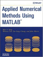
Figure 1.8 The graphs of a sinc function defined by sinc1().
>>D = 0.5; b1 = -2; b2 = 2; t = b1+[0:200]/200*(b2 - b1);
>>plot(t,sinc1(t,D)), axis([b1 b2 -0.4 1.2])
>>hold on, plot(t,sinc1(t),’k:’)
The two plotting commands coupled with sinc1(t,D) and sinc1(t) yield the
two beautiful graphs, respectively, as depicted in Fig. 1.8a. It is important to
note that
sinc1() doesn’t bother us and works fine without the second input
argument
D. We owe the second line in the function sinc1() for the nice error-
handling service:
if nargin < 2,D=1;end
This line takes care of the case where the number of input arguments (nargin)is
less than 2, by assuming that the second input argument is
D=1by default. This
programming technique is the key to making the MATLAB functions adaptive
to different number/type of input arguments, which is very useful for breathing
the user-convenience into the MATLAB functions. To appreciate its role, we
remove the second line from the M-file defining

sinc1() and then type the same
statement in the Command window, trying to use
sinc1() without the second
input argument.
>>plot(t,sinc1(t),’k:’)
??? Input argument ’D’ is undefined.
Error in ==> C:\MATLAB6p5\nma\sinc1.m
On line 4 ==> x = sin(pi*t/D)./(pi*t/D);
This time we get a serious (red) error message with no graphic result. It is implied
that the MATLAB function without the appropriate error-handling parts no longer
allows the user’s default or carelessness.
Now, consider the third line in
sinc1(), which is another error-handling state-
ment.
t(find(t==0))=eps;
TOWARD GOOD PROGRAM 43
or, equivalently
for i = 1:length(t), if t(i) == 0, t(i) = eps; end, end
This statement changes every zero element in the t vector into eps (2.2204e-
016). What is the real purpose of this statement? It is actually to remove the
possibility of division-by-zero in the next statement, which is a mathematical
expression having
t in the denominator.
x = sin(pi*t/D)./(pi*t/D);
To appreciate the role of the third line in sinc1(), we remove it from the M-file
defining
sinc1(), and type the following statement in the Command window.
>>plot(t,sinc1(t,D),’r’)
Warning: Divide by zero.
(Type "warning off MATLAB:divideByZero" to suppress this warning.)

In C:\MATLAB6p5\nma\sinc1.m at line 4)
This time we get just a warning (black) error message with a similar graphic
result as depicted in Fig. 1.8b. Does it imply that the third line is dispensable?
No, because the graph has a (weird) hole at t = 0, about which most engi-
neers/mathematicians would feel uncomfortable. That’s why authors strongly
recommend you not to omit such an error-handling part as the third line as
well as the second line in the MATLAB function
sinc1().
(cf) What is the value of sinc1(t,D) for t=0in this case? Aren’t you curious? If so,
let’s go for it.
>>sinc1(0,D), sin(pi*0/D)/(pi*0/D), 0/0
ans = NaN (Not-a-Number: undetermined)
Last, consider of the fourth line in sinc1(), which is only one essential
statement performing the main job.
x = sin(pi*t/D)./(pi*t/D);
What is the . (dot) before /(division operator) for? In reference to this, authors
gave you a piece of advice that you had better put a .(dot) just before the
arithmetic operators
*(multiplication), /(division), and ^(power) in the function
definition so that the term-by-term (termwise) operation can be done any time
(Section 1.1.6, (A5)). To appreciate the existence of the
.(dot), we remove it from
the M-file defining
sinc1(), and type the following statements in the Command
window.
>>clf, plot(t,sinc1(t,D)), sinc1(t,D), sin(pi*t/D)/(pi*t/D)
ans = -0.0187
44 MATLAB USAGE AND COMPUTATIONAL ERRORS
What do you see in the graphic window on the screen? Surprise, a (horizontal)
straight line running parallel with the t-axis far from any sinc function graph!

What is more surprising, the value of
sinc1(t,D) or sin(pi*t/D)/(pi*t/D)
shows up as a scalar. Authors hope that this accident will help you realize how
important it is for right term-by-term operations to put .(dot) before the arithmetic
operators
*, / and ^ . By the way, aren’t you curious about how MATLAB deals
with a vector division without .(dot)? If so, let’s try with the following statements:
>>A = [1:10]; B = 2*A; A/B, A*B’*(B*B’)^-1, A*pinv(B)
ans = 0.5
To understand this response of MATLAB, you can see Section 1.1.7 or Sec-
tion 2.1.2.
In this section we looked a t several sources of runtime error, hoping that it
aroused the reader’s attention to the danger of runtime error.
1.3.5 Parameter Sharing via Global Variables
When we discuss the runtime error that may be caused by user’s default in passing
some parameter as input argument to the corresponding function, you might feel
that the parameter passing job is troublesome. Okay, it is understandable as a
beginner in MATLAB. How about declaring the parameters as global so that
they can be accessed/shared from anywhere in the MATLAB world as far as the
declaration is valid? If you want to, you can declare any varable(s) by inserting
the following statement in both the main program and all the functions using
the variables.
global Gravity_Constant Dielectric_Constant
%plot_sinc
clear, clf
global D
D=1;b1=-2;b2=2;
t = b1 +[0:100]/100*(b2 - b1);
%passing the parameter(s) through arguments of the function
subplot(221), plot(t, sinc1(t,D))

axis([b1 b2 -0.4 1.2])
%passing the parameter(s) through global variables
subplot(222), plot(t, sinc2(t))
axis([b1 b2 -0.4 1.2])
function x = sinc1(t,D)
if nargin<2, D = 1; end
t(find(t == 0)) = eps;
x = sin(pi*t/D)./(pi*t/D);
function x = sinc2(t)
global D
t(find(t == 0)) = eps;
x = sin(pi*t/D)./(pi*t/D);
Then, how convenient it would be, since you don’t have to bother about pass-
ing the parameters. But, as you get proficient in programming and handle many
TOWARD GOOD PROGRAM 45
functions/routines that are involved with various sets of parameters, you might
find that the global variable is not always convenient, because of the follow-
ing reasons.
ž
Once a variable is declared as global, its value can be changed in any of the
MATLAB functions having declared it as global, without being noitced by
other related functions. Therefore it is usual to declare only the constants as
global and use long names (with all capital letters) as their names for easy
identification.
ž
If some variables a re declared as global and modified by several func-
tions/routines, it is not easy to see the relationship and the interaction among
the related functions in terms of the global variable. In other words, the pro-
gram readability gets worse as the number of global variables and related
functions increases.

For example, let us look over the above program “plot
sinc.m” and the func-
tion “
sinc2()”. They both have a declaration of D as global; consequently,
sinc2() does not need the second input argument for getting the parameter
D. If you run the program, you will see that the two plotting statements adopting
sinc1() and sinc2() produce the same graphic r esult as depicted in Fig. 1.8a.
1.3.6 Parameter Passing Through Varargin
In this section we see two kinds of routines that get a function name (string)
with its parameters as its input argument and play with the function.
First, let us look over the routine “
ez_plot1()”, which gets a function name
(
ftn) with its parameters (p) and the lower/upper bounds (bounds = [b1 b2])
as its first, third, and second input argument, respectively, and plots the graph of
the given function over the interval set by the bounds. Since the given function
may or may not have its parameter, the two cases are determined and processed
by the number of input arguments (
nargin)intheif-else-end block.
%plot_sinc1
clear, clf
D=1;b1=-2;b2=2;
t = b1+[0:100]/100*(b2 - b1);
bounds = [b1 b2];
subplot(223), ez_plot1(’sinc1’,bounds,D)
axis([b1 b2 -0.4 1.2])
subplot(224), ez_plot(’sinc1’,bounds,D)
axis([b1 b2 -0.4 1.2])
function ez_plot1(ftn,bounds,p)
if nargin < 2, bounds = [-1 1]; end

b1 = bounds(1); b2 = bounds(2);
t = b1+[0:100]/100*(b2 - b1);
if nargin <= 2, x = feval(ftn,t);
else x = feval(ftn,t,p);
end
plot(t,x)
function
ez_plot(ftn,bounds,varargin)
if nargin < 2, bounds = [-1 1]; end
b1 = bounds(1); b2 = bounds(2);
t = b1 + [0:100]/100*(b2 - b1);
x = feval(ftn,t,varargin{:});
plot(t,x)
46 MATLAB USAGE AND COMPUTATIONAL ERRORS
Now, let us see the routine “ez_plot()”, which does the same plotting job
as “
ez_plot1()”. Note that it has a MATLAB keyword varargin (variable
length argument list) as its last input argument and passes it into the MATLAB
built-in function
feval() as its last input argument. Since varargin can repre-
sent comma-separated multiple parameters including expression/strings, it paves
the highway for passing the parameters in relays. As the number of parame-
ters increases, it becomes much more convenient to use
varargin for passing
the parameters than to deal with the parameters one-by-one as in
ez_plot1().
This technique will be widely used later in Chapter 4 (on nonlinear equations),
Chapter 5 (on numerical integration), Chapter 6 (on ordinary differential equa-
tions), and Chapter 7 (on optimization).
(cf) Note that MATLAB has a built-in graphic function ezplot(), which is much more

powerful and convenient to use than
ez_plot(). You can type ‘help ezplot’tosee
its function and usage.
1.3.7 Adaptive Input Argument List
A MATLAB function/routine is said to be “adaptive” to users in terms of input
arguments if it accepts different number/type of input arguments and makes a
reasonable interpretation. For example, let us see the nonlinear equation solver
routine ‘
newton()’ in Section 4.4. Its input argument list is
(f,df,x0,tol,kmax)
where f, df, x0, tol and kmax denote the filename (string) of function (to
be solved), the filename (string) of its derivative function, the initial guess (for
solution), the error tolerance and the maximum number of iterations, respectively.
Suppose the user, not knowing the derivative, tries to use the routine w ith just
four input arguments as follows.
>>newton(f,x0,tol,kmax)
At first, these four input arguments will be accepted as f,df,x0, and tol,
respectively. But, when the second line of the program body is executed, the
routine will notice something wrong from that
df is not any filename but a
number and then interprets the input arguments as
f,x0,tol, and kmax to the
idea of the user. This allows the user to use the routine in two ways, depending
on whether he is going to supply the routine with the derivative function or not.
This scheme is conceptually quite similar to function overloading of C++, but
C++ requires us to have several functions having the same name, with different
argument list.
PROBLEMS
1.1 Creating a Data File and Retrieving/Plotting Data Saved in a Data File
(a) Using the MATLAB editor, make a program “

nm1p01a”, which lets its
user input data pairs of heights [ft] and weights [lb] of as many persons
PROBLEMS 47
as he wants until he presses <Enter> and save the whole data in the
form of an N ×2matrixintoanASCIIdatafile(
***.dat) named by
the user. If you have no idea how to compose such a program, you
can permutate the statements in the box below to make your program.
Store the program in the file named “nm1p01a.m” and run it to save
the following data into the data file named “hw.dat”:
5.5162
6.1185
5.7170
6.5195
6.2191
%nm1p01a: input data pairs and save them into an ASCII data file
clear
k=0;
while 1
end
k=k+1;
x(k,1) = h;
h = input(’Enter height:’)
x(k,2) = input(’Enter weight:’)
if isempty(h), break; end
cd(’c:\matlab6p5\work’) %change current working directory
filename = input(’Enter filename(.dat):’,’s’);
filename = [filename ’.dat’]; %string concatenation
save(filename,’x’,’/ascii’)
(b) Make a MATLAB program “nm1p01b”, which reads (loads) the data

file “hw.dat” made in (a), plots the data as in F ig. 1.1a in the upper-
left region of the screen divided into four regions like Fig. 1.3, and
plots the data in the form of piecewise-linear (PWL) graph describing
the relationship between the height and the weight in the upper-right
region of the screen. Let each data pair be denoted by the symbol ‘+’
on the graph. Also let the ranges of height and w eight be [5, 7] and
[160, 200], respectively. If you have no idea, you can permutate the
statements in the below box. Additionally, run the program to check if
it works fine.
%nm1p01b: to read the data file and plot the data
cd(’c:\matlab6p5\work’) %change current working directory
weight = hw(I,2);
load hw.dat
clf, subplot(221)
plot(hw)
subplot(222)
axis([5 7 160 200])
plot(height,weight,height,weight,’+’)
[height,I] = sort(hw(:,1));
48 MATLAB USAGE AND COMPUTATIONAL ERRORS
1.2 Text Printout of Alphanumeric Data
Make a routine
max_array(A), which uses the max() command to find one
of the maximum elements of a matrix
A given as its input argument and
uses the
fprintf() command to print it onto the screen together with its
row/column indices in the following format.
’\n Max(A) is A(%2d,%2d) = %5.2f\n’,row_index,col_index,maxA
Additionally, try it to have the maximum element of an arbitrary matrix

(generated by the following two consecutive commands) printed in this
format onto the screen.
>>rand(’state’,sum(100*clock)), rand(3)
1.3 Plotting the Mesh Graph of a Two-Dimensional Function
Consider the MATLAB program “
nm1p03a”, whose objective is to draw
a cone.
(a) The statement on the sixth line seems to be dispensable. Run the pro-
gram with and without this line and see what happens.
(b) If you want to plot the function fcone(x,y) defined in another M-file
‘
fcone.m’, how will you modify this program?
(c) If you replace the fifth line by ‘
Z = 1-abs(X)-abs(Y);’, what differ-
ence does it make?
%nm1p03a: to plot a cone
clear, clf
x = -1:0.02:1; y = -1:0.02:1;
[X,Y] = meshgrid(x,y);
Z = 1-sqrt(X.^2+Y.^2);
Z = max(Z,zeros(size(Z)));
mesh(X,Y,Z)
function z = fcone(x,y)
z = 1-sqrt(x.^2 + y.^2);
1.4 Plotting The Mesh Graph of Stratigraphic Structure
Consider the incomplete MATLAB program “
nm1p04”, whose objective is
to draw a stratigraphic structure of the area around Pennsylvania State
University from the several perspective point of view. The data about
the depth of the rock layer at 5 × 5 sites are listed in Table P1.4. Sup-

plement the incomplete parts of the program so that it serves the pur-
pose and run the program to answer the following questions. If you com-
plete it properly and run it, MATLAB will show you the four similar
graphs at the four corners of the screen and be waiting for you to press
any key.
PROBLEMS 49
(a) At whatvalue of k does MATLAB show you the mesh/surface-type graphs
that are the most similar to the first graphs? From this result, what do you
guess are the default values of the azimuth or horizontal rotation angle and
the vertical elevation angle (in degrees) of the perspective view point?
(b) As the first input argument
Az of the command view(Az,E1) decreases,
in which direction does the perspective viewpoint revolve round the
z-axis, clockwise or counterclockwise (seen from the above)?
(c) As the second input argument
El of the command view(Az,E1) increases,
does the perspective viewpoint move up or down along the z-axis?
(d) What is the difference between the plotting commands
mesh() and
meshc()?
(e) What is the difference between the usages of the command
view()
with two input arguments Az,El and with a three-dimensional vector
argument
[x,y,z]?
Table P1.4 The Depth of the Rock Layer
x Coordinate
y Coordinate 0.1 1.2 2.5 3.6 4.8
0.5 410 390 380 420 450
1.4 395 375 410 435 455

2.2 365 405 430 455 470
3.5 370 400 420 445 435
4.6 385 395 410 395 410
%nm1p04: to plot a stratigraphic structure
clear, clf
x = [0.1 . ];
y = [0.5 . ];
Z = [410 390 ];
[X,Y] = meshgrid(x,y);
subplot(221), mesh(X,Y,500 - Z)
subplot(222), surf(X,Y,500 - Z)
subplot(223), meshc(X,Y,500 - Z)
subplot(224), meshz(X,Y,500 - Z)
pause
for k = 0:7
Az = -12.5*k; El = 10*k; Azr = Az*pi/180; Elr = El*pi/180;
subplot(221), view(Az,El)
subplot(222),
k, view([sin(Azr),-cos(Azr),tan(Elr)]), pause %pause(1)
end
1.5 Plotting a Function over an Interval Containing Its Singular Point Noting
that the tangent function f(x) = tan(x) is singular at x = π/2, 3π/2, let us
plot its graph over [0, 2π] as follows.
50 MATLAB USAGE AND COMPUTATIONAL ERRORS
(a) Define the domain vector x consisting of sufficiently many intermediate
point x
i
’s along the x-axis and the corresponding vector y consisting
of the function values at x
i

’s and plot the vector y over the vector x.
You may use the following statements.
>>x = [0:0.01:2*pi]; y = tan(x);
>>subplot(221), plot(x,y)
Which one is the most similar to what you have got, among the graphs
depicted in Fig. P1.5? Is it far from your expectation?
(b) Expecting to get the better graph, we scale it up along the y-axis by
using the following command.
>>axis([0 6.3 -10 10])
Which one is the most similar to what you have got, among the graphs
depicted in Fig. P1.5? Is it closer to your expectation than what you
got in (a)?
(c) Most probably, you must be nervous about the straight lines at the
singular points x = π/2andx = 3π/2. The more disturbed you become
by the lines that must not be there, the better you are at the numerical
stuffs. As an alternative to a void such a singular happening, you can
try dividing the interval into three sections excluding the two singular
points as follows.
024
(a) (b)
(c)
6
−500
500
1000
1500
0
0246
−10
0

5
10
−5
0246
−10
0
5
10
−5
Figure P1.5 Plotting the graph of f(x) = tan x.
PROBLEMS 51
>>x1 = [0:0.01:pi/2-0.01]; x2 = [pi/2+0.01:0.01:3*pi/2-0.01];
>>x3 = [3*pi/2+0.01:0.01:2*pi];
>>y1 = tan(x1); y2 = tan(x2); y3 = tan(x3);
>>subplot(222), plot(x1,y1,x2,y2,x3,y3), axis([0 6.3 -10 10])
(d) Try adjusting the number of intermediate points within the plotting
interval as follows.
>>x1 = [0:200]*pi/100; y1 = tan(x1);
>>x2 = [0:400]*pi/200; y2 = tan(x2);
>>subplot(223), plot(x1,y1), axis([0 6.3 -10 10])
>>subplot(224), plot(x2,y2), axis([0 6.3 -10 10])
From the difference between the two graphs you got, you might have
guessed that it would be helpful to increase the number of intermediate
points. Do you still have the same idea even after you adjust the range
of the y-axis to [−50, +50] by using the following command?
>>axis([0 6.3 -50 50])
(e) How about trying the easy plotting command ezplot()? Does it answer
your desire?
>>ezplot(’tan(x)’,0,2*pi)
1.6 Plotting the Graph of a Sinc Function

The sinc function is defined as
f(x) =
sin x
x
(P1.6.1)
whose value at x = 0is
f(0) = lim
x→0
sin x
x
=
(sin x)

x





x=0
=
cos x
1



x=0
= 1 (P1.6.2)
We are going to plot the graph of this function over [−4π, +4π ].
(a) Casually, you may try as follows.

>>x = [-100:100]*pi/25; y = sin(x)./x;
>>plot(x,y), axis([-15 15 -0.4 1.2])
In spite of the warning message about ‘division-by-zero’, you may
somehow get a graph. But, is there anything odd about the graph?
(b) How about trying with a different domain vector?
>>x = [-4*pi:0.1:+4*pi]; y = sin(x)./x;
>>plot(x,y), axis([-15 15 -0.4 1.2])
52 MATLAB USAGE AND COMPUTATIONAL ERRORS
Surprisingly, MATLAB gives us the function values without any com-
plaint and presents a nice graph of the sinc function. What is the
difference between (a) and (b)?
(cf) Actually, we would have no problem if we used the MATLAB built-in function
sinc().
1.7 Termwise (Element-by-Element) Operation in In-Line Functions
(a) Let the function f
1
(x) be defined without one or both of the dot(.)
operators in Section 1.1.6. Could we still get the output vector consist-
ing of the function values for the several values in the input vector?
You can type the following statements into the MATLAB command
window and see the results.
>>f1 = inline(’1./(1+8*x^2)’,’x’); f1([0 1])
>>f1 = inline(’1/(1+8*x.^2)’,’x’); f1([0 1])
(b) Let the function f
1
(x) be defined with both of the dot(.) operators as in
Section 1.1.6. What would we get by typing the f ollowing statements
into the MATLAB command window?
>>f1 = inline(’1./(1+8*x.^2)’,’x’); f1([0 1]’)
1.8 In-Line Function and M-file Function with the Integral Routine ‘quad()’

As will be seen in Section 5.8, one of the MATLAB built-in functions for
computing the integral is ‘
quad()’, the usual usage of w hich is
quad(f,a,b,tol,trace,p1,p2, ) for

b
a
f(x,p1,p2, )dx
(P1.8.1)
where
f is the name of the integrand function (M-file name should be categorized
by
’’)
a,b are the lower/upper bound of the integration interval
tol is the error tolerance (10
−6
by default [])
trace setto1(on)/0(off)(0bydefault[]) for subintervals
p1,p2, are additional parameters to be passed directly to function f
Let’s use this
quad() routine with an in-line function and an M-file function
to obtain

m+10
m−10
(x −x
0
)f (x)dx (P1.8.2a)
and


m+10
m−10
(x −x
0
)
2
f(x)dx (P1.8.2b)
PROBLEMS 53
where
x
0
= 1,f(x)=
1
√
2πσ
e
−(x−m)
2
/2σ
2
with m = 1,σ = 2 (P1.8.3)
Below are an incomplete main program ‘
nm1p08’ and an M-file function
defining the integrand of (P1.8.2a). Make another M-file defining the inte-
grand of ( P1.8.2b) and complete the main program to compute the two
integrals (P1.8.2a) and (P1.8.2b) by using the in-line/M-file functions.
function xfx = xGaussian_pdf(x,m,sigma,x0)
xfx = (x - x0).*exp(-(x - m).^2/2/sigma^2)/sqrt(2*pi)/sigma;
%nm1p08: to try using quad() with in-line/M-file functions
clear

m = 1; sigma = 2;
int_xGausspdf = quad(’xGaussian_pdf’,m - 10,m + 10,[],0,m,sigma,1)
Gpdf = ’exp(-(x-m).^2/2/sigma^2)/sqrt(2*pi)/sigma’;
xGpdf = inline([’(x - x0).*’ Gpdf],’x’,’m’,’sigma’,’x0’);
int_xGpdf = quad(xGpdf,m - 10,m+10,[],0,m,sigma,1)
1.9 µ-Law Function Defined in an M-File
The so-called µ-law function and µ
−1
-law function used for non-uniform
quantization is defined as
y = g
µ
(x) =|y|
max
ln(1 + µ|x|/|x|
max
)
ln(1 + µ)
sign(x) (P1.9a)
x = g
−1
µ
(y) =|x|
max
(1 +µ)
|y|/|y|
max
− 1
µ
sign(y) (P1.9b)

Below are the µ-law function
mulaw() defined in an M-file and a main
program
nm1p09, which performs the following jobs:
ž
Finds the values y of the µ-law function for x = [-1:0.01:1], plots the
graph of
y versus x.
ž
Finds the values x0 of the µ
−1
-law function for y.
ž
Computes the discrepancy between x and x0.
Complete the µ
−1
-law function mulaw_inv() and store it together with
mulaw() and nm1p09 in the M-files named “mulaw inv.m”, “mulaw.m”,
and “nm1p09.m”, respectively. Then run the main program
nm1p09 to plot
the graphs of the µ-law function with µ = 10, 50 and 255 and find the
discrepancy between
x and x0.
54 MATLAB USAGE AND COMPUTATIONAL ERRORS
function [y,xmax] = mulaw(x,mu,ymax)
xmax = max(abs(x));
y = ymax*log(1+mu*abs(x/xmax))./log(1+mu).*sign(x); % Eq.(P1.9a)
function x = mulaw_inv(y,mu,xmax)
%nm1p09: to plot the mulaw curve
clear, clf

x = [-1:.005:1];
mu = [10 50 255];
for i = 1:3
[y,xmax] = mulaw(x,mu(i),1);
plot(x,y,’b-’, x,x0,’r-’), hold on
x0 = mulaw_inv(y,mu(i),xmax);
discrepancy = norm(x-x0)
end
1.10 Analog-to-Digital Converter (ADC)
Below are two ADC routines
adc1(a,b,c) and adc2(a,b,c), which assign
the corresponding digital value
c(i) to each one of the analog data belong-
ing to the quantization interval [
b(i), b(i+1)]. Let the boundary vector
and the centroid vector be, respectively,
b=[-3-2-10123]; c=[-2.5 -1.5 -0.5 0.5 1.5 2.5];
(a) Make a program that uses two ADC routines to find the output d for
the analog input data
a = [-300:300]/100 and plots d versus a to see
the input-output relationship of the ADC, which is supposed to be like
Fig. P1.10a.
function d = adc1(a,b,c)
%Analog-to-Digital Converter
%Input a = analog signal, b(1:N + 1) = boundary vector
c(1:N)=centroid vector
%Output: d = digital samples
N = length(c);
for n = 1:length(a)
I = find(a(n) < b(2:N));

if ~isempty(I), d(n) = c(I(1));
else d(n) = c(N);
end
end
function d=adc2(a,b,c)
N = length(c);
d(find(a < b(2))) = c(1);
for i = 2:N-1
index = find(b(i) <=a&a<=b(i+1)); d(index) = c(i);
end
d(find(b(N) <= a)) = c(N);
PROBLEMS 55
input
output
4
2
0
−2
−4
−4 −20
(a) The input-output relationship of an ADC
24
time
analog input
digital
output
024
(b) The output of an ADC to a sinusoidal input
68
Figure P1.10 The characteristic of an ADC (analog-to-digital converter).

(b) Make a program that uses two ADC routines to find the output d for
the analog input data
a = 3*sin(t) with t = [0:200]/100*pi and
plots
a and d versus t to see how the analog input is converted into the
digital output by the ADC. The graphic result is supposed to be like
Fig. P1.10b.
1.11 Playing with Polynomials
(a) Polynomial Evaluation:
polyval()
Write a MATLAB statement to compute
p(x) = x
8
− 1forx = 1 (P1.11.1)
(b) Polynomial Addition/Subtraction by Using Compatible Vector Addi-
tion/Subtraction
Write a MATLAB statement to add the following two polynomials:
p
1
(x) = x
4
+ 1,p
2
(x) = x
3
− 2x
2
+ 1 (P1.11.2)
(c) Polynomial Multiplication:
conv()

Write a MATLAB statement to get the following product of polynomials:
p(x) = (x
4
+ 1)(x
2
+ 1)(x +1)(x − 1)(P1.11.3)
(d) Polynomial Division:
deconv()
Write a MATLAB statement to get the quotient and the remainder of
the following polynomial division:
p(x) = x
8
/(x
2
− 1)(P1.11.4)
(e) Routine for Differentiation/Integration of a Polynomial
What you see in the below box is the r outine “
poly_der(p)”, which
gets a polynomial coefficient vector
p (in the descending order) and
outputs the coefficient vector
pd of its derivative polynomial. Likewise,
you can make a routine “
poly_int(p)”, which outputs the coefficient
56 MATLAB USAGE AND COMPUTATIONAL ERRORS
vector of the integral polynomial for a given polynomial coefficient
vector.
(cf) MATLAB has the built-in routines polyder()/polyint() for finding the
derivative/integral of a polynomial.
function pd = poly_der(p)

%p: the vector of polynomial coefficients in descending order
N = length(p);
if N <= 1, pd = 0; % constant
else
fori=1:N-1,pd(i) = p(i)*(N - i); end
end
(f) Roots of A Polynomial Equation: roots()
Write a MATLAB statement to get the roots of the following polynomial
equation
p(x) = x
8
− 1 = 0 (P1.11.5)
You can check if the result is right, by using the MATLAB command
poly(), which generates a polynomial having a given set of roots.
(g) Partial Fraction Expansion of a Ratio of Two Polynomials:
residue()/
residuez()
(i) The MATLAB routine [r,p,k] = residue(B,A) finds the partial
fraction expansion for a ratio of given polynomials B(s)/A(s) as
B(s)
A(s)
=
b
1
s
M−1
+ b
2
s
M−2

+···+b
M
a
1
s
N−1
+ a
2
s
N−2
+···+a
N
= k(s) +

i
r(i)
s −p(i)
(P1.11.6a)
which is good for taking the inverse Laplace transform. Use this
routine to find the partial fraction expansion for
X(s) =
4s +2
s
3
+ 6s
2
+ 11s +6
=
s +
+

s +
+
s +
(P1.11.7a)
(ii) The MATLAB routine
[r,p,k] = residuez(B,A) finds the par-
tial fraction expansion for a ratio of given polynomials B(z)/A(z)
as
B(z)
A(z)
=
b
1
+ b
2
z
−1
+···+b
M
z
−(M−1)
a
1
+ a
2
z
−1
+···+a
N
z

−(N−1)
= k(z
−1
) +

i
r(i)z
z − p(i)
(P1.11.6b)
which is good for taking the inverse z-transform. Use this routine
to find the partial fraction e xpansion for
X(z) =
4 +2z
−1
1 + 6z
−1
+ 11z
−2
+ 6z
−3
=
z
z +
+
z
z +
+
z
z +
(P1.11.7b)

PROBLEMS 57
(h) Piecewise Polynomial: mkpp()/ppval()
Suppose we have an M × N matrix P, the rows of which denote
M (piecewise) polynomials of degree (N − 1) for different (non-
overlapping) intervals with
(M+1) boundary points bb = [b(1)
b(M + 1)]
, where the polynomial coefficients in each row are
supposed to be generated with the interval starting from x = 0. Then
we can use the MATLAB command
pp = mkpp(bb,P) to construct a
structure of piecewise polynomials, which can be evaluated by using
ppval(pp).
Figure P1.11(h) shows a set of piecewise polynomials {p
1
(x +3),
p
2
(x +1), p
3
(x − 2)} for the intervals [−3, −1],[−1, 2] and [2, 4],
respectively, where
p
1
(x) = x
2
,p
2
(x) =−(x −1)
2

, and p
3
(x) = x
2
− 2 (P1.11.8)
Make a MATLAB program which uses
mkpp()/ppval() to plot this
graph.
0
p
1
(
x
+ 3) = (
x
+ 3)
2
p
3
(
x
− 2) = (
x
− 2)
2
−2
p
2
(
x

+ 1) = −
x

2
−3
−5
0
5
−2 −1 123
x
4
Figure P1.11(h) The graph of piecewise polynomial functions.
(cf) You can type ‘help mkpp’ to see a couple o f examples showing the usage
of
mkpp.
1.12 Routine for Matrix Multiplication
Assuming that MATLAB cannot perform direct multiplication on vectors/
matrices, supplement the following incomplete routine “
multiply_matrix
(A,B)
” so that it can multiply two matrices given as its input arguments only
if their dimensions are compatible, but displays an error message if their
dimensions are not compatible. Try it to get the product of two arbitrary
3 ×3 matrices generated by the command
rand(3) and compare the result
with that obtained by using the direct multiplicative operator
*. Note that
58 MATLAB USAGE AND COMPUTATIONAL ERRORS
the matrix multiplication can be described as
C(m, n) =

K

k=1
A(m, k)B(k,n) (P1.12.1)
function C = multiply_matrix(A,B)
[M,K] = size(A); [K1,N] = size(B);
if K1 ~= K
error(’The # of columns of A is not equal to the # of rows of B’)
else
form=1:
forn=1:
C(m,n) = A(m,1)*B(1,n);
fork=2:
C(m,n) = C(m,n) + A(m,k)*B(k,n);
end
end
end
end
1.13 Function for Finding Vector Norm
Assuming that MATLAB does not have the
norm() command finding us the
norm of a given vector/matrix, make a routine
norm_vector(v,p),which
computes the norm of a given vector as
||v||
p
=
p





N

n=1
|v
n
|
p
(P1.13.1)
for any positive integer
p, finds the maximum absolute value of the elements
for
p = inf and computes the norm as if p=2, even if the second input
argument
p is not given. If you have no idea, permutate the statements in the
below box and save it in the file named “
norm_vector.m”. Additionally, try
it to get the norm with
p=1,2,∞ (inf) and of an arbitrary vector generated
by the command
rand(2,1). Compare the result with that obtained by using
the
norm() command.
function nv = norm_vector(v,p)
if nargin < 2, p = 2; end
nv = sum(abs(v).^p)^(1/p);
nv = max(abs(v));
ifp>0&p~=inf
elseif p == inf

end
PROBLEMS 59
1.14 Backslash(\) Operator
Let’s play with the backslash(
\) operator.
(a) Use the backslash(
\) command, the minimum-norm solution (2.1.7) and
the
pinv() command to solve the following equations, find the residual
error ||A
i
x −b
i
||’s and the rank of the coefficient matrix A
i
,andfillin
Table P1.14 with the results.
(i) A
1
x =

123
456



x
1
x
2

x
3


=

6
15

= b
1
(P1.14.1)
(ii) A
2
x =

123
246



x
1
x
2
x
3


=


6
8

= b
2
(P1.14.2)
(iii) A
3
x =

123
246



x
1
x
2
x
3


=

6
12

= b

3
(P1.14.3)
Table P1.14 Results of Operations with backslash (\)Operatorandpinv( ) Command
backslash(\) Minimum-Norm or
LS Solution
pinv() Remark
on rank(A
i
)
redundant/x ||A
i
x − b
i
|| x ||A
i
x − b
i
|| x ||A
i
x − b
i
||
inconsistent
1.5000 4.4409e-15
A
1
x = b
1
0 (1.9860e-15)
1.5000

0.3143 1.7889
A
2
x = b
2
0.6286
0.9429
A
3
x = b
3
A
4
x = b
4
2.5000 1.2247
0.0000
A
5
x = b
5
A
6
x = b
6
(cf) When the mismatching error ||A
i
x − b
i
||’s obtained from MATLAB 5.x/6.x version are slightly different, the

former one is in the parentheses ().
60 MATLAB USAGE AND COMPUTATIONAL ERRORS
(b) Use the backslash (\) command, the LS (least-squares) solution (2.1.10)
and the
pinv() command to solve the following equations and find the
residual error ||A
i
x − b
i
||’s and the rank of the coefficient matrix A
i
,
and fill in Table P1.14 with the results.
(i) A
4
x =


12
23
34



x
1
x
2

=



2
6
7


= b
4
(P1.14.4)
(ii) A
5
x =


12
24
36



x
1
x
2

=


1

5
8


= b
5
(P1.14.5)
(iii) A
6
x =


12
24
36



x
1
x
2

=


3
6
9



= b
6
(P1.14.6)
(cf) If some or all of the rows of the coefficient matrix A in a set of linear equations
can be expressed as a linear combination o f other row(s), the corresponding
equations are dependent, which can be revealed by the rank deficiency, that is,
rank(A) < min(M, N) where M and N are the row dimension and the column
dimension, respectively. If some equations are dependent, they may have either
inconsistency (no exact solution) or redundancy (infinitely many solutions),
which can be distinguished by checking if augmenting the RHS vector b to the
coefficient matrix A increases the rank or not—that is, rank([A b]) > rank(A)
or not [M-2].
(c) Based on the results obtained in (a) and (b) and listed in Table P1.14,
answer the following questions.
(i) Based on the results obtained in (a)(i), which one yielded the
non-minimum-norm solution among the three methods, that is,
the backslash(
\) operator, the minimum-norm solution (2.1.7) and
the
pinv() command? Note that the minimum-norm solution
means the solution whose norm (||x||) is the minimum over the
many solutions.
(ii) Based on the results obtained in (a), which one is most reliable
as a means of finding the minimum-norm solution among the
three methods?
(iii) Based on the results obtained in (b), choose two reliable methods
as a means of finding the LS (least-squares) solution among the
three methods, that is, the backslash (
\) operator, the LS solu-

tion (2.1.10) and the
pinv() command. Note that the LS solution
PROBLEMS 61
means the solution for which the residual error (||Ax − b||)isthe
minimum over the many solutions.
1.15 Operations on Vectors
(a) Find the mathematical expression for the computation to be done by
the following MATLAB statements.
>>n = 0:100; S = sum(2.^-n)
(b) Write a MATLAB statement that performs the following computation.

10000

n=0
1
(2n + 1)
2

−
π
2
8
(c) Write a MATLAB statement which uses the commands
prod() and
sum() to compute the product of the sums of each row of a 3 × 3
random matrix.
(d) How does the following MATLAB routine “
repetition(x,M,m)” con-
vert a given row vector sequence
x to make a new sequence y ?

function y = repetition(x,M,m)
ifm==1
MNx = ones(M,1)*x; y = MNx(:)’;
else
Nx = length(x); N = ceil(Nx/m);
x = [x zeros(1,N*m - Nx)];
MNx = ones(M,1)*x;
y = [];
for n = 1:N
tmp = MNx(:,(n - 1)*m + [1:m]).’;
y = [y tmp(:).’];
end
end
(e) Make a MATLAB routine “zero_insertion(x,M,m)”, which inserts
m zeros just after every Mth element of a given row vector sequence
x to make a new sequence. Write a MATLAB statement to apply the
routine for inserting two zeros just after every third element of
x =
[
137249
]toget
y = [
1370024900
]
(f) How does the following MATLAB routine “
zeroing(x,M,m)” convert
a given row vector sequence
x to make a new sequence y?
62 MATLAB USAGE AND COMPUTATIONAL ERRORS
function y = zeroing(x,M,m)

%zero out every (kM - m)th element
if nargin < 3, m = 0; end
if M<=0,M=1;end
m = mod(m,M);
Nx = length(x); N = floor(Nx/M);
y = x; y(M*[1:N] - m) = 0;
(g) Make a MATLAB routine “sampling(x,M,m)”, which samples every
(
kM-m)th element of a given row vector sequence x tomakeanew
sequence. Write a MATLAB statement to apply the routine for sampling
every (3k − 2)th element of x = [
137249
]toget
y = [1 2]
(h) Make a MATLAB routine ‘
rotation_r(x,M)”, which rotates a given
row vector sequence
x right by M samples, say, making rotate_r([1
2 3 4 5],3) = [34512]
.
1.16 Distribution of a Random Variable: Histogram
Make a routine
randu(N,a,b), which uses the MATLAB function rand()
to generate an N-dimensional random vector having the uniform distribution
over [
a, b] and depicts the graph for the distribution of the elements of
the generated vector in the f orm of histogram divided into 20 sections as
Fig.1.7. Then, see what you get by typing the following statement into the
MATLAB command window.
>>randu(1000,-2,2)

What is the height of the histogram on the average?
1.17 Number Representation
In Section 1.2.1, we looked over how a number is represented in 64 bits.
For example, the IEEE 64-bit floating- point number system represents the
number 3(2
1
≤ 3 < 2
2
) belonging to the range R
1
= [2
1
, 2
2
) with E = 1as
0 100 0000 0000 0000 0000 . . . . . . . . . . . . 0000 0000 0000 0000 0000
000000 . . . . . . . .00048
1000
where the exponent and the mantissa are
Exp = E + 1023 = 1 + 1023 = 1024 = 2
10
= 100 0000 0000
M = (3 × 2
−E
− 1) × 2
52
= 2
51
= 1000 0000 0000 0000 0000 0000 0000 0000
PROBLEMS 63

This can be confirmed by typing the following statement into MATLAB
command window.
>>fprintf(’3 = %bx\n’,3) or >>format hex, 3, format short
which will print out onto the screen
0000000000000840 4008000000000000
Noting that more significant byte (8[bits] = 2[hexadecimal digits]) of a
number is stored in the memory of higher a ddress number in the INTEL
system, we can reverse the order of the bytes in this number to see the
number having the most/least significant byte on the left/right side as we
can see in the daily life.
00 00 00 00 00 00 08 40 → 40 08 00 00 00 00 00 00
This is exactly the hexadecimal representation of the number 3 as we
expected. You can find the IEEE 64-bit floating-point number represen-
tation of the number 14 and use the command
fprintf() or format hex to
check if the result is right.
<procedure of adding 2
−1
to 2
3
> <procedure of subtracting 2
−1
from 2
3
>
alignment
right result
truncation of guard bit
1 .0000 × 2
3

+ 1 .0000 × 2
−1
.00000 × 2
3
.00010 × 2
3
alignment
2’s
complement
1 .0000 × 2
3
− 1 .0000 × 2
−1
1 .0000 0 × 2
3
− 0 .00010 × 2
3
1 .00000 × 2
3
+ 1 .11110 × 2
3
1 .00010 × 2
3
1 .0001 × 2
3
= (1 + 2
−4
) × 2
3
right result

normalization
truncation of guard bit
0 .11110 × 2
3
1 .1110 × 2
2
= (1 + 1 − 2
−3
) × 2
2
<procedure of adding 2
−2
to 2
3
>
alignment
.0000 × 2
3
+ 1 .0000 × 2
−2
1 .00000 × 2
3
+ 0 .0000 1 × 2
3
no difference
truncation of guard bit
: hidden bit,
(cf)
1 .00001 × 2
3

1 .0000 × 2
3
= (1 + 0) × 2
3
<procedure of subtracting 2
−2
from 2
3
>
alignment
1 .0000 × 2
3
− 1 .0000 × 2
−2
1 .00000 × 2
3
− 0 .00001 × 2
3
1 .00000 × 2
3
+ 1 .11111 × 2
3
2’s
complement
right result
normalization
truncation of guard bit
0 .11111 × 2
3
1 .1111 × 2

2
= (1 + 1 − 2
−4
) × 2
2
1
+ 0
1
: guard bit
Figure P1.18 Procedure of addition/subtraction with four mantissa bits.
1.18 Resolution of Number Representation and Quantization Error
In Section 1.2.1, we have seen that adding 2
−22
to 2
30
makes some dif-
ference, while adding 2
−23
to 2
30
makes no difference due to the bit shift
by over 52 bits for alignment before addition. How about subtracting 2
−23
from 2
30
? In contrast with the addition of 2
−23
to 2
30
, it makes a differ-

ence as you can see by typing the following statement into the MATLAB
64 MATLAB USAGE AND COMPUTATIONAL ERRORS
command window.
>>x = 2^30;x+2^-23==x,x-2^-23==x
which will give you the logical answer 1 (true) and 0 (false). Justify this
result based on the difference of resolution of two ranges [2
30
,2
31
)and[2
29
,
2
30
) to which the true values of c omputational results (2
30
+ 2
−23
)and(2
30
−
2
−23
) belong, respectively. Note from Eq. (1.2.5) that the resolutions—that is,
the maximum quantization errors—are 
E
= 2
E−52
= 2
−52+30

= 2
−22
and
2
−52+29
= 2
−23
, respectively. For details, r efer to Fig. P1.18, which illustrates
the procedure of addition/subtraction with four mantissa bits, one hidden bit,
and one guard bit.
1.19 Resolution of Number Representation and Quantization Error
(a) What is the result of typing the following statements into the MATLAB
command window?
>>7/100*100 - 7
How do you compare the absolute value of this answer w ith the reso-
lution  of the range to which 7 belongs?
(b) Find how many numbers are susceptible to this kind of quantization
error caused by division/multiplication by 100, among the numbers
from 1 to 31.
(c) What will be the result of running the following program? Why?
%nm1p19: Quantization Error
x = 2-2^-50;
for n = 1:2^3
x = x+2^-52; fprintf(’%20.18E\n’,x)
end
1.20 Avoiding Large Errors/Overflow/Underflow
(a) For x = 9.8
201
and y = 10.2
199

, evaluate the following two expressions
that are mathematically equivalent and tell which is better in terms of
the power of resisting the overflow.
(i) z =

x
2
+ y
2
(P1.20.1a)
(ii) z = y

(x/y)
2
+ 1 (P1.20.1b)
Also for x = 9.8
−201
and y = 10.2
−199
, evaluate the above two expres-
sions and tell which is better in terms of the power of resisting the
underflow.
(b) With a = c = 1 and for 100 values of b over the interval [10
7.4
,10
8.5
]
generated by the MATLAB command ‘
logspace(7.4,8.5,100)’,
PROBLEMS 65

evaluate the following two formulas (for the roots of a quadratic
equation) that are mathematically equivalent and plot the values of the
second root of each pair. Noting that the true values are not available
and so the shape of solution graph is only one practical basis on which
we can assess the quality of numerical solutions, tell which is better in
terms of resisting the loss of significance.
(i)

x
1
,x
2
=
1
2a
(−b ∓ sign(b)
√
b
2
− 4ac)

(P1.20.2a)
(ii)

x
1
=
1
2a
(−b − sign(b)

√
b
2
− 4ac),x
2
=
c/a
x
1

(P1.20.2b)
(c) For 100 values of x over the interval [10
14
,10
16
], evaluate the follow-
ing two expressions that are mathematically equivalent, plot them, and
based on the graphs, tell which is better in terms of resisting the loss
of significance.
(i) y =
√
2x
2
+ 1 − 1 (P1.20.3a)
(ii) y =
2x
2
√
2x
2

+ 1 + 1
(P1.20.3b)
(d) For 100 values of x over the interval [10
−9
,10
−7.4
], evaluate the fol-
lowing two expressions that are mathematically equivalent, plot them,
and based on the graphs, tell which is better in terms of resisting the
loss of significance.
(i) y =
√
x +4 −
√
x +3 (P1.20.4a)
(ii) y =
1
√
x +4 +
√
x +3
(P1.20.4b)
(e) On purpose to find the value of (300
125
/125!)e
−300
, type the following
statement into the MATLAB command window.
>>300^125/prod([1:125])*exp(-300)
What is the result? Is it of any help to change the order of multipli-

cation/division? As an alternative, make a routine which evaluates the
expression
p(k) =
λ
k
k!
e
−λ
for λ = 300 and an integer k(P1.20.5)
in a recursive way, say, like p(k + 1) = p(k) ∗ λ/k and then, use the
routine to find the value of (300
125
/125!)e
−300
.
66 MATLAB USAGE AND COMPUTATIONAL ERRORS
(f) Make a routine w hich computes the sum
S(K) =
K

k=0
λ
k
k!
e
−λ
for λ = 100 and an integer K(P1.20.6)
and then, use the routine to find the value of S(155).
1.21 Recursive Routines for Efficient Computation
(a) The Hermite Polynomial [K-1]

Consider the Hermite polynomial defined as
H
0
(x) = 1,H
N
(x) = (−1)
N
e
x
2
d
N
dx
N
e
−x
2
(P1.21.1)
(i) Show that the derivative of this polynomial function can be writ-
ten as
H

N
(x) = (−1)
N
2xe
x
2
d
N

dx
N
e
−x
2
+ (−1)
N
e
x
2
d
N+1
dx
N+1
e
−x
2
= 2xH
N
(x) − H
N+1
(x) (P1.21.2)
and so the (N + 1)th-degree Hermite polynomial can be obtained
recursively from the Nth-degree Hermite polynomial as
H
N+1
(x) = 2xH
N
(x) − H


N
(x) (P1.21.3)
(ii) Make a MATLAB routine “
Hermitp(N)” which uses Eq. (P1.21.3)
to generate the Nth-degree Hermite polynomial H
N
(x).
(b) The Bessel F unction of the First Kind [K-1]
Consider the Bessel function of the first kind of order k defined as
J
k
(β) =
1
π

π
0
cos(kδ −β sin δ)dδ (P1.21.4a)
=

β
2

k
∞

m=0
(−1)
m
β

2m
4
m
m!(m + k)!
≡ (−1)
k
J
−k
(β) (P1.21.4b)
(i) Define the integrand of (P1.21.4a) in the name of ‘
Bessel_inte-
grand(x,beta,k)
’ and store it in an M-file named “Bessel_
integrand.m
”.
(ii) Complete the following routine “
Jkb(K,beta)”, which uses
(P1.21.4b) in a recursive way to compute J
k
(β) of order k =
1:K for given K and β (beta).
(iii) Run the following program
nm1p21b which uses Eqs. (P1.21.4a)
and (P1.21.4b) to get J
15
(β) for β = 0:0.05:15. What is the norm