Software Fault Tolerance Techniques and Implementation phần 7 docx
Bạn đang xem bản rút gọn của tài liệu. Xem và tải ngay bản đầy đủ của tài liệu tại đây (950.88 KB, 35 trang )
•
The executive discards the checkpoint and clears the WDT; the
results are passed outside the RtB, and the RtB is exited.
5.1.1.3 Primarys Results Are On Time, but Fail Acceptance Test; Successful
Execution with Re-Expressed Inputs
Now lets look at what happens if 2 executes without exception and its results
are sent to the AT, but they do not pass the AT. If the deadline for acceptable
results has not expired and a new DRA option is available, the inputs are re-
expressed and the primary is executed with the new input data. Differences
between this scenario and the failure-free scenario are in gray type. This sce-
nario is similar to the previous scenario, except for the cause of 2 s initial
failure.
•
Upon entry to the RtB, the executive performs the following: a
checkpoint (or recovery point) is established, a call to 2 is formatted,
and the WDT is set to WP.
• 2 is executed. No exception or time-out occurs during execution
of 2.
• The results of 2 are submitted to the AT.
•
2 s results fail the AT.
•
Control returns to the executive. The executive checks to ensure the
deadline for acceptable results has not expired (it has not in this sce-
nario) and checks if there is a(nother) DRA option available that has
not been attempted on this input (there is one available).
•
The executive restores the checkpoint, then calls the DRA with the
original input data as its argument.
•
The executive formats a call to 2 using the re-expressed input.
•
2 is executed. No exception or time-out occurs during execution of
2 with the re-expressed input.
•
The results of 2 are submitted to the AT.
•
2 s results are on time and pass the AT.
•
Control returns to the executive.
•
The executive discards the checkpoint and clears the WDT; the
results are passed outside the RtB, and the RtB is exited.
196 Software Fault Tolerance Techniques and Implementation
TEAMFLY
Team-Fly
®
5.1.1.4 All Data Re-Expression Algorithm Options Are Used Without Success;
Successful Backup Execution
This scenario examines the case when the deadline expires without an accept-
able result or when all DRA options fail. This may occur if the combined
execution time of the P(DRA
i
(x)), i = 1, 2, … number of DRA, is too long
(versus individual algorithm time-outs) or when the DRA results are input
to P and executed, and their results continue to fail the AT. If there are no
DRA options remaining and no primary algorithm result has been accepted,
the backup algorithm is invoked and, in this scenario, passes its AT (i.e.,
ATB). Differences between this scenario and the failure-free scenario are in
gray type.
•
Upon entry to the RtB, the executive performs the following: a
checkpoint (or recovery point) is established, a call to P is formatted,
and the WDT is set to WP.
•
P is executed. No exception or time-out occurs during execution
of P.
• The results of P are submitted to the AT.
• P s results fail the AT.
• Control returns to the executive. The executive checks to ensure the
deadline for acceptable results has not expired (it has not) and
checks if there is a(nother) DRA option available that has not been
attempted on this input (there is one available).
•
The executive restores the checkpoint, then calls DRA
1
with the
original input data as its argument.
•
The executive formats a call to P using the re-expressed input.
•
P is executed. No exception or time-out occurs during execution of
P with this re-expressed input.
•
The results of P are submitted to the AT.
•
P s results are on time, but fail the AT.
•
Control returns to the executive. The executive checks to ensure
the deadline for acceptable results has not expired (it has not) and
checks if there is a(nother) DRA option available that has not been
attempted on this input (there is one available).
•
The executive restores the checkpoint, then calls DRA
2
with the
original input data as its argument.
•
The executive formats a call to P using the re-expressed input.
Data Diverse Software Fault Tolerance Techniques 197
•
P is executed. No exception or time-out occurs during execution of
P with this re-expressed input.
•
The results of P are submitted to the AT.
•
P s results are on time, but fail the AT.
•
Control returns to the executive. The executive checks to ensure
the deadline for acceptable results has not expired (it has not) and
checks if there is a(nother) DRA option available that has not been
attempted on this input (there are no additional DRA options
available).
•
The executive restores the checkpoint, formats a call to the backup,
B, using the original inputs, and invokes B.
•
B is executed. No exception occurs during execution of B.
•
The results of B are submitted to the ATB.
• B s results are on time and pass the ATB.
•
Control returns to the executive.
• The executive discards the checkpoint, clears the WDT, the results
are passed outside the RtB, and the RtB is exited.
5.1.1.5 All Data Re-Expression Algorithm Options Are Used Without Success;
Backup Executes, but Fails Backup Acceptance Test
This scenario examines the case when the deadline expires without an accept-
able result or when all DRA options fail. This may occur if the combined
execution time of the P(DRA
i
(x)), i = 1, 2, … number of DRA is too long
(versus individual algorithm time-outs) or when the DRA results are input to
P and executed and their results continue to fail the AT. If there are no DRA
options remaining and no primary algorithm result has been accepted,
the backup algorithm is invoked. In this scenario, the backup fails its AT (the
ATB). A failure exception is raised and the RtB is exited. Differences
between this scenario and the failure-free scenario are in gray type.
•
Upon entry to the RtB, the executive performs the following: a
checkpoint (or recovery point) is established, a call to P is formatted,
and the WDT is set to WP.
•
P is executed. No exception or time-out occurs during execution
of P.
•
The results of P are submitted to the AT.
198 Software Fault Tolerance Techniques and Implementation
•
P s results fail the AT.
•
Control returns to the executive. The executive checks to ensure
the deadline for acceptable results has not expired (it has not) and
checks if there is a(nother) DRA option available that has not been
attempted on this input (there is one available).
•
The executive restores the checkpoint, then calls DRA
1
with the
original input data as its argument.
•
The executive formats a call to P using the re-expressed input.
•
P is executed. No exception or time-out occurs during execution of
P with this re-expressed input.
•
The results of P are submitted to the AT.
•
P s results are on time, but fail the AT.
•
Control returns to the executive. The executive checks to ensure
the deadline for acceptable results has not expired (it has not) and
checks if there is a(nother) DRA option available that has not been
attempted on this input (there is one available).
• The executive restores the checkpoint, then calls DRA
2
with the
original input data as its argument.
•
The executive formats a call to P using the re-expressed input.
•
P is executed. No exception or time-out occurs during execution of
P with this re-expressed input.
•
The results of P are submitted to the AT.
•
P s results are on time, but fail the AT.
•
Control returns to the executive. The executive checks to ensure the
deadline for acceptable results has not expired (it has not) and
checks if there is a(nother) DRA option available that has not been
attempted on this input (there are no additional DRA options avail-
able).
•
The executive restores the checkpoint, formats a call to the backup,
B, using the original inputs, and invokes B.
•
B is executed. No exception occurs during execution of B.
•
The results of B are submitted to the ATB.
•
B s results are on time, but fail the ATB.
•
Control returns to the executive.
Data Diverse Software Fault Tolerance Techniques ''
•
The executive discards the checkpoint and clears the WDT; a failure
exception is raised, and the RtB is exited.
5.1.1.6 Augmentations to Retry Block Technique Operation
We have seen in these scenarios that the RtB operation continues until
acceptable results are produced, there are no new DRA options to try and the
backup fails, or the deadline expires without an acceptable result from either
the primary or the backup.
Several augmentations to the RtB can be imagined. One is to use a
DRA execution counter. This counter is used when the primary fails on the
original input and primary execution is attempted with re-expressed inputs.
This counter indicates the maximum number of times to execute the primary
with different re-expressed inputs. The counter is incremented once the pri-
mary fails and prior to each execution with re-expressed input. The benefit
of using the DRA execution counter is that it provides the ability to have a
means of imposing a deadline without using a timer. However, the coun-
ter cannot detect execution failure or infinite loops within the primary. This
type of failure can be detected by a watchdog type of augmentation timer
(recall Section 4.1 for its use with the RcB technique).
The RtB technique may also be augmented by the use of a more
detailed AT comprised of several tests, as described in Section 4.1.1.5 in
conjunction with the RcB technique. Also, notice in the scenarios that we
denoted a different AT for the backup algorithm, ATB. If the backup algo-
rithm is significantly different from the primary or if its functionality
includes additional measures to ensure graceful degradation, for example, it
may be necessary to use a different AT than that of the primary. However, if
the primary and backup are developed based on the same specification and
required functionality, then the same AT can be used for both variants.
We also indicated in the scenarios that there is at least one DRA and
perhaps multiple DRA options. This possibly awkward wording was used
because there can either be a single DRA that can re-express an input in mul-
tiple ways or multiple DRAs to use. This is illustrated in Figure 5.2.
With the multiple DRA, a different algorithm is used in each case:
DRA
i
(x)
j
, where
i = the DRA algorithm number;
j = number of the pass within the RtB technique.
200 Software Fault Tolerance Techniques and Implementation
Note that with the single DRA, something within the DRA must result in a
different re-expression of the input on each use of the algorithm. This could
be implemented using a random number generator, a conditional switch
implementing a different algorithm or by providing a different algorithm
parameter (other than the input x), and so on.
Data Diverse Software Fault Tolerance Techniques 201
DRA
x
DRA( )x
1
DRA ( )
1 1
x
DRA ( )
2 2
x
DRA( )x
2
DRA( )x
n
DRA ( )
n n
x
DRA
x
DRA
x
DRA
1
x
DRA
2
x
DRA
n
x
nth use of DRA during execution within RtB block
2nd use of DRA during execution within RtB block
1st use of DRA during execution within RtB block
DRA( ) DRA( ) ,x x j k
j k
≠ ≠ DRA ( ) DRA ( ) ,
i j i k
x x j k≠ ≠
Figu re 5.2 Multiuse singl e versus multiple d ata re-exp ression algorithms.
5.1.2 Retry Block Example
Lets look at an example for the RtB technique. Suppose the original pro-
gram uses inputs N and O, where N and O are measured by sensors with a toler-
ance of ±0.02. Also, suppose the original algorithm should not receive an
input of N = 0.0 because of the nature of the algorithm. However, the values
of N can be very close to zero (see Figure 5.3 illustrating B (N, O)). For example,
if the program receives the input (1.5, 1.2), it operates correctly and pro-
duces a correct result. However, suppose that if it receives input close to
N = 0.0, such as (1A
−10
, 2.2), lack of precision in the data type used causes
storage of the N value to be zero, and causes a divide-by-zero error in the
program.
Figure 5.4 illustrates an approach to using retry blocks with this prob-
lem. Note the additional components needed for RtB technique imple-
mentation: an executive that handles checkpointing and orchestrating the
technique, a DRA, a backup sort algorithm, and an AT. In this example, no
WDT is used. The AT in this example is a simple bounds test; that is, the
result is accepted if B (N, O) ≥ 100.0.
Now, lets step through the example.
• Upon entry to the RtB, the executive establishes a checkpoint and
formats calls to the primary and backup routines. The input is
(1A
−10
, 2.2).
•
The primary algorithm, B (N, O), is executed and results in a divide-
by-zero error.
202 Software Fault Tolerance Techniques and Implementation
O
N
0
Potential
÷ 0 error
domain
Figu re 5.3 Exam ple input space.
• An exception is raised and is handled by the RtB executive. The
executive sets a flag indicating failure of the primary algorithm using
the original inputs and restores the checkpoint.
•
The executive formats a call to the DRA to re-express the original
inputs.
•
The DRA, R(x) = x + 0.0021, modifies the x input parameter
within x s limits of accuracy.
•
The executive formats a call to the primary algorithm with the
re-expressed inputs.
•
The primary algorithm executes and returns the result 123.45.
•
The result is submitted to the AT. The result is greater than or equal
to 100.0, so the result of the primary algorithm using re-expressed
inputs passes the AT.
•
Control returns to the executive.
•
The executive discards the checkpoint, the results are passed outside
the RtB, and the RtB is exited.
Data Diverse Software Fault Tolerance Techniques 203
Checkpoint
Primary algorithm
( , )B N O
Restore checkpoint
÷ 0 error
using original
inputs
DRA 1: ( )4 N
1
=
N + 0.0021
AT:B N O( , )
100.0≥
Pass
(1A
−10
, 2.2)
123.45 using
re-expressed
inputs
(1A
−10
+ 0.0021, 2.2)
Figu re 5.4 Exam ple of retry block implementation.
5.1.3 Retry Block Issues and Discussion
This section presents the advantages, disadvantages, and issues related to
the RtB technique. In general, software fault tolerance techniques provide
protection against errors in translating requirements and functionality into
code, but do not provide explicit protection against errors in specifying
requirements. This is true for all of the techniques described in this book.
Being a data diverse, backward recovery technique, the RtB technique
subsumes data diversitys and backward recoverys advantages and disadvan-
tages, too. These are discussed in Sections 2.3 and 1.4.1, respectively. While
designing software fault tolerance into a system, many considerations have to
be taken into account. These are discussed in Chapter 3. Issues related to
several software fault tolerance techniques (such as similar errors, coincident
failures, overhead, cost, redundancy, etc.) and the programming practices
used to implement the techniques are described in Chapter 3. Issues related
to implementing ATs are discussed in Section 7.2.
There are a few issues to note specifically for the RtB technique. The
RtB technique runs in a sequential (uniprocessor) environment. When the
results of the primary with original inputs pass the AT, the overhead incurred
(beyond that of running the primary alone, as in non-fault-tolerant software)
includes setting the checkpoint and executing the AT. If, however, these
results fail the AT, then the time overhead also includes the time for recover-
ing the checkpointed information, execution time for each DRA (or each
pass through a single DRA), execution times for each time the primary is run
with re-expressed inputs until one passes the AT (or until all attempts fail the
AT), and run-time of the AT each time results are checked. It is assumed that
most of the time the primarys first-execution results will pass the AT, so the
expected time overhead is that of setting the checkpoint and executing the
AT. This is little beyond the primarys execution time (unless an unusually
large amount of information is being checkpointed). In the worst case, how-
ever, the RtB techniques execution time is the sum of all the module execu-
tions mentioned above (in the case where the primarys results fail the AT).
This wide variation in execution time exposes the RtB to timing errors that
may be unacceptable for real-time applications. One solution to the overhead
problem is the distributed recovery block (DRB) (see Section 4.3) in which
the modules and AT are executed in parallel, modified for use with data
diverse program elements.
In RtB operation, when executing DRAs and re-executing the primary,
the service that the module is to provide is interrupted during the recovery.
204 Software Fault Tolerance Techniques and Implementation
This interruption may be unacceptable in applications that require high
availability.
One advantage of the RtB technique is that it is naturally applicable to
software modules, as opposed to whole systems. It is natural to apply RtB
to specific critical modules or processes in the system without incurring the
cost and complexity of supporting fault tolerance for an entire system.
Simple, highly effective DRAs and ATs are required for effective RtB
technique operation. The success of data diverse software fault tolerance
techniques depends on the performance of the re-expression algorithm used.
Several ways to perform data re-expression and insight on actual re-
expression algorithms and their use are presented in Sections 2.3.1 through
2.3.3. DRAs are very application dependent, with their development requir-
ing in-depth knowledge of the algorithm. Development of DRAs also
requires a careful analysis of the type and magnitude of re-expression appro-
priate for each candidate datum [3]. There is no general rule for the deriva-
tion of DRAs for all applications; however, this can be done for some special
cases [10] and they do exist for a fairly wide range of applications [11]. A
simple DRA is more desirable than a complex one because the simpler algo-
rithm is less likely to contain design faults.
A simple, effective AT can also be difficult to develop and depends
heavily on the specification (see Section 7.2). If an error is not detected
by the AT (or by the other error detection mechanisms), then that error is
passed along to the module that receives the retry blocks results and will not
trigger any recovery mechanisms.
Both RcB and RtB techniques can suffer the domino effect (Sec-
tion 3.1.3), in which cascaded rollbacks can push all processes back to their
beginnings. This occurs if recovery and communication operations are not
coordinated, especially in the case of nested recovery or retry blocks.
Not all applications can employ data diversity; however, many real-
time control systems and other applications can use DRAs. For example, sen-
sors typically provide noisy and imprecise data, so small modifications to that
data would not adversely affect the application [1] and can yield a means of
implementing fault tolerance. The performance of the DRA itself is much
more important to program dependability than the technique structure (such
as NCP, RtB, and others) in which it is embedded [12].
The RtB technique provides data diversity, but not design diversity.
This may limit the techniques ability to tolerate some fault types. The use
of combination design and data diverse techniques (see Section 5.3 for
Data Diverse Software Fault Tolerance Techniques #
example) may assist in overcoming this limitation, but more research and
experimentation is required.
To implement the RtB technique, the developer can use the pro-
gramming techniques (such as assertions, checkpointing, atomic actions)
described in Chapter 3. Also needed for implementation and further exami-
nation of the technique is information on the underlying architecture and
performance. These are discussed in Sections 5.1.3.1 and 5.1.3.2, respec-
tively. Table 5.1 lists several RtB technique issues, indicates whether or not
they are an advantage or disadvantage (if applicable), and points to where in
the book the reader may find additional information.
The indication that an issue in the above table can be a positive or
negative (+/−) influence on the technique or on its effectiveness further indi-
cates that the issue may be a disadvantage in general (e.g., cost is higher than
non-fault-tolerant software) but an advantage in relation to another tech-
nique. In these cases, the reader is referred to the discussion of the issue.
206 Software Fault Tolerance Techniques and Implementation
Table 5.1
Retry Block Issue Summary
Issue
Advantage (+)/
Disadvantage (−) Where Discussed
Provides protection against errors in trans lating
requirements and functionalit y into code (true for
software fault tolerance techniques in g eneral)
+ Chapter 1
Does not prov ide explicit protection against errors in
specifying req uirements (true for software fault
tolerance techniques in gene ral)
− Chapter 1
General backwa rd recovery advantages + Section 1.4.1
General backwa rd recovery disadvantages − Section 1.4.1
General data diversity advantages + Section 2.3
General data diversity disadvantages − Section 2.3
DRA +/− Sections 2.3.12.3.3
Similar errors or common residual design errors − Section 3.1.1
Coincident and correlated failures − Section 3.1.1
Domino effect − Section 3.1.3
Space and time redundancy +/− Section 3.1.4
Dependability studies +/− Section 4.1.3.3
ATs and discussions related to specific types of ATs +/− Section 7.2
TEAMFLY
Team-Fly
®
5.1.3.1 Architecture
We mentioned in Sections 1.3.1.2 and 2.5 that structuring is required if we
are to handle system complexity, especially when fault tolerance is involved
[1315]. This includes defining the organization of software modules onto
the hardware elements on which they run. The RtB approach is typically
uniprocessor, with all components residing on a single hardware unit. All
communications between the software components is done through function
calls or method invocations in this architecture.
5.1.3.2 Performance
There have been numerous investigations into the performance of software
fault tolerance techniques in general (discussed in Chapters 2 and 3) and the
dependability of specific techniques themselves. Table 4.2 (Section 4.1.3.3)
provides a list of references for these dependability investigations. This list,
although not exhaustive, provides a good sampling of the types of analyses
that have been performed and substantial background for analyzing software
fault tolerance dependability. Ammann and Knight provide a model to
determine the success of an RtB system in [3]. The reader is encouraged
to examine all references (in Table 4.2 and otherwise) for details on assump-
tions made by the researchers, experiment design, and results interpretation.
The fault tolerance of a system employing data diversity depends upon
the ability of the DRA to produce data points outside of a failure region,
given an initial data point that is within a failure region. The program exe-
cutes correctly on re-expressed data points only if they are outside a failure
region. If the failure region has a small cross section in some dimensions,
then re-expression should have a high probability of translating the data
point out of the failure region.
5.2 N-Copy Programming
NCP, also developed by Ammann and Knight [13], is the other (along with
RtB) original data diverse software fault tolerance technique. NCP is a data
diverse technique, and is further categorized as a static technique (described
in Section 4.2). The hardware fault tolerance architecture related to the NCP
is N-modular or static redundancy. The processes can run concurrently on
different computers or sequentially on a single computer, but in practice,
they are typically run concurrently. NCP is the data diverse complement of
N-version programming (NVP).
Data Diverse Software Fault Tolerance Techniques 207
The NCP technique uses a decision mechanism (DM) (see Section 7.1)
and forward recovery (see Section 1.4.2) to accomplish fault tolerance. The
technique uses one or more DRAs (see Sections 2.3.1 through 2.3.3) and at
least two copies of a program. The system inputs are run through the DRA(s)
to re-express the inputs. The copies execute in parallel using the re-expressed
data as input (each input is different, one of which may be the original input
value). A DM examines the results of the copy executions and selects the
best result, if one exists. There are many alternative DMs available for use
with NCP.
NCP operation is described in 5.2.1, with an example provided in
5.2.2. The advantages and disadvantages of the NCP technique are presented
in 5.2.3.
5.2.1 N-Copy Programming Operation
The basic NCP technique consists of an executive, 1 to n DRA, n copies of
the program or function, and a DM. The executive orchestrates the NCP
technique operation, which has the general syntax:
run DRA 1, DRA 2, …, DRA
n
run Copy 1(result of DRA 1),
Copy 2(result of DRA 2),
…,
Copy
n
(result of DRA
n
)
if (Decision Mechanism (Result 1, Result 2,
…,
Result
n
))
return Result
else failure exception
The NCP syntax above states that the technique first runs the DRA
concurrently to re-express the input data, then executes the n copies concur-
rently. The results of the copy executions are provided to the DM, which
operates upon the results to determine if a correct result can be adjudicated.
If one can (i.e., the
Decision Mechanism statement above evaluates to
TRUE), then it is returned. If a correct result cannot be determined, then an
error occurs.
Figure 5.5 illustrates the structure and operation of the NCP tech-
nique. As shown, n copies of a program execute in parallel, each on a differ-
ent set of re-expressed data. If the re-expression algorithm used is exact (that
is, all copies should generate identical outputs), then a conventional majority
voter can be used. If an approximate re-expression algorithm is used, the n
copies could produce different but acceptable outputs, and an enhanced DM
208 Software Fault Tolerance Techniques and Implementation
(such as the formal majority voter, Section 7.1.5) is needed. (Exact and
approximate re-expression algorithms are defined in Section 2.3.2.)
Both fault-free and failure scenarios (one in which a correct result can-
not be found and one that fails prior to reaching the DM) for the NCP are
described below. In examining these scenarios, the following abbreviations
will be used:
C
i
Copy i;
DM Decision mechanism;
DRA
i
Data re-expression algorithm i;
n The number of copies;
NCP N-copy programming;
R
i
Result of C
i
;
x Original input;
y
i
Re-expressed input, y
i
= DRA
i
(x), i = 1, …, n.
Data Diverse Software Fault Tolerance Techniques 209
NCP entry NCP
Exception raised
Output selected
Distribute
inputs
Copy 2
DM
NCP exit Failure exception
Gather
results
Copy nCopy 1
DRA 2 DRA nDRA 1
Figu re 5.5 N-co py program ming structure and operation.
5.2.1.1 Failure-Free Operation
This scenario describes the operation of NCP when no failure or exception
occurs.
•
Upon entry to NCP, the executive sends the input, x, to the n DRA
to be re-expressed.
•
The DRA run their re-expression algorithms (exact DRA, in this
example) on x, yielding the re-expressed inputs y
i
= DRA
i
(x).
•
The executive gathers the re-expressed input, formats calls to the n
copies and through those calls distributes the re-expressed inputs to
the copies.
•
Each copy, C
i
, executes. No failures occur during their execution.
•
The results of the copy executions (R
i
, i = 1, …, n) are gathered by
the executive and submitted to the exact majority DM.
•
The R
i
are equal to one another, so the DM selects R
2
(randomly,
since the results are equal), as the correct result.
• Control returns to the executive.
• The executive passes the correct result outside the NCP, and the
NCP module is exited.
5.2.1.2 Failure ScenarioIncorrect Results
This scenario describes the operation of NCP when the DM cannot deter-
mine a correct result. Differences between this scenario and the failure-free
scenario are in gray type.
•
Upon entry to NCP, the executive sends the input, x, to the n DRA
to be re-expressed.
•
The DRA run their re-expression algorithms (exact DRA, in this
example) on x, yielding the re-expressed inputs y
i
= DRA
i
(x).
•
The executive gathers the re-expressed input, formats calls to the n
copies and through those calls distributes the re-expressed inputs to
the copies.
•
Each copy, C
i
, executes.
•
The results of the copy executions (R
i
, i = 1, …, n) are gathered by
the executive and submitted to the exact majority DM.
210 Software Fault Tolerance Techniques and Implementation
•
None of the R
i
are equal. The DM cannot determine a correct result,
and it sets a flag indicating this fact.
•
Control returns to the executive.
•
The executive raises an exception and the NCP module is exited.
5.2.1.3 Failure ScenarioCopy Does Not Execute
This scenario describes the operation of NCP when at least one copy does
not complete its execution. Differences between this scenario and the
failure-free scenario are in gray type.
•
Upon entry to NCP, the executive sends the input, x, to the n DRA
to be re-expressed.
•
The DRA run their re-expression algorithms (exact DRA here) on x,
yielding the re-expressed inputs y
i
= DRA
i
(x).
• The executive gathers the re-expressed input, formats calls to the n
copies, and through those calls distributes the re-expressed inputs to
the copies.
• The copies, C
i
, begin execution. One or more copies do not com-
plete execution for some reason (e.g., stuck in an endless loop).
•
The executive cannot retrieve all copy results in a timely manner.
The executive submits the results it does have to the DM.
•
The DM expects n results, but receives n-1 (or n-2, etc., depend-
ing on the number of failed copies) results. The basic exact majority
voter cannot handle fewer than n results and sets a flag indicating
its failure to select a correct result. (Note: If the DM is not equipped
to recognize this failure, it may fail, and the executive would have
to recognize the DM failure.)
•
Control returns to the executive.
•
The executive raises an exception and the NCP module is exited.
5.2.1.4 Augmentations to N-Copy Programming Operation
We have seen in these scenarios that NCP operation continues until the DM
adjudicates a correct result, the DM cannot select a correct result, or the
DM itself fails. It is also evident how similar the operations are of the NVP
and NCP techniques.
Data Diverse Software Fault Tolerance Techniques 211
Augmentations to the basic NCP can involve using a different DM
than the basic majority voter. Chapter 7 describes several alternatives. One
optional DM is the dynamic voter (Section 7.1.6). Its ability to handle a vari-
able number of result inputs could tolerate the failure experienced in the last
scenario above.
Another augmentation to basic NCP involves voting on the results
as each copy completes execution (as opposed to waiting on all copies to
complete). Once two results are available, the DM can compare them and, if
they agree, complete that NCP cycle. If the first two results do not match,
the DM performs a majority vote on three results when it receives the third
copys results, and continues voting through the nth copy execution, until it
finds an acceptable result. When an acceptable result is found, it is passed
outside the NCP, any remaining copy executions are terminated, and the
NCP module is exited. This scheme provides results more quickly than the
basic NCP only if it is possible that one or more copies have different execu-
tion times based on the input received.
The DRA used with the NCP technique are application dependent,
but there is room for variety in their design. Several example DRA are
described in Section 2.3.3.
Another augmentation, this one via combination with other tech-
niques, has been made to the NCP technique. This is the TPA described
later in this chapter.
5.2.2 N-Copy Programming Example
This section provides an example implementation of the NCP technique.
Suppose the original program uses inputs x and y, where x and y are measured
by sensors with a tolerance of ±0.02. Also, suppose the original algorithm
should not receive an input of x = 0.0 because of the nature of the algo-
rithm. However, the values of x can be very close to zero (see Figure 5.3 in
Section 5.1.2 illustrating f (x, y)). For example, if the program receives the
input (1.5, −1.2), it operates correctly and produces a correct result. How-
ever, suppose that if it receives input close to x = 0.0, such as (1e
−10
, 2.2), lack
of precision in the data type used causes storage of the x value to be zero, and
causes a divide-by-zero error in the program.
Figure 5.6 illustrates an ex ample NCP implementation of the
example problem. Note the additional components needed for NCP imple-
mentationan executive that handles orchestrating and synchronizing
the technique, one or more DRA, one or more additional copies of the
algorithm/program, and a DM. In this example, three DRAs are used: a
212 Software Fault Tolerance Techniques and Implementation
pass-through DRA, which simply forwards the original inputs without modi-
fication; a DRA that adds 0.002 (recall the tolerance for x) to the input; and
a DRA that adds 0.001 to the input. These re-expressed inputs are sent to the
algorithm copies. The copies perform their functions on the inputs and the
voter determines the correct result. In this case, a majority voter using toler-
ances is applied. (Note that the voter tolerance is a different entity than the
inputs tolerance.) As suspected, the original input produces a divide-by-zero
error. But the other DRA/copy pairs produce results that are equal within a
tolerance of 0.75 and pass the voter. (See Chapter 7 for more information on
tolerance voters.)
Now, lets step through the example.
•
Upon entry to NCP, the executive sends the input, (1e
−10
, 2.2), to
the three DRAs to be re-expressed.
•
The DRAs run their re-expression algorithms on the input yielding
the following re-expressed inputs:
DRA
1
(1e
−10
, 2.2) = (1e
−10
, 2.2) Pass-through DRA
Data Diverse Software Fault Tolerance Techniques 213
Distribute
inputs
(1
e
−10
, 2.2)
DRA 2:
R x x
2
( ) 0.002= +
DRA 3:
R x x
3
( ) 0.001= +
DRA 1:
Pass-through
( )R x x
1
=
(1e
−
10
, 2.2)
Copy 1:
( , )f x y
Copy 2:
( , ) 123.45f x y =
(0.002 + 1 , 2.2)e
−
10
(0.001 + 1 , 2.2)e
−
10
Copy 3:
( , ) 123.96f x y =
DM:
Majority tolerance 0.75, =
123.96 − 123.45 0.51 0.75= <
÷ 0 error
123.45
123.96
123.45
∅
Figu re 5.6 Example of N-copy progr amming imp lementation.
DRA
2
(1e
−
10
, 2.2) = (0.002 + 1e
−
10
, 2.2)
DRA
3
(1e
−
10
, 2.2) = (0.001 + 1e
−
10
, 2.2)
•
The executive gathers the re-expressed inputs, formats calls to the
n = 3 copies and through those calls distributes the re-expressed
inputs to the copies.
•
Each copy, C
i
(i = 1, 2, 3), executes.
•
The results of the copy executions (r
i
, i = 1, …, n) are gathered by
the executive and submitted to the DM.
•
The DM examines the results:
Copy r
i
Decision Mechanism Algorithm
1 ∅ (divide-by-zero error )
2
123.45 | 123.45 1 23.96 | = 0.51 < 0.75 (where 0.75 is
the DM tolerance)
3 123.96
The adjudicated result is 123.45 (randomly selected from those copy
results matching within the tolerance).
•
Control returns to the executive.
•
The executive passes the correct result, 123.45, outside the NCP,
and the NCP module is exited.
5.2.3 N-Copy Programming Issues and Discussion
This section presents the advantages, disadvantages, and issues related to
NCP. As stated earlier, software fault tolerance techniques generally provide
protection against errors in translating requirements and functionality into
code, but do not provide explicit protection against errors in specifying
requirements. This is true for all of the techniques described in this
book. Being a data diverse, forward recovery technique, NCP subsumes data
diversitys and forward recoverys advantages and disadvantages, too. These
are discussed in Sections 2.3 and 1.4.2, respectively. While designing soft-
ware fault tolerance into a system, many considerations have to be taken into
account. These are discussed in Chapter 3. Issues related to several soft-
ware fault tolerance techniques (such as, similar errors, overhead, cost,
redundancy, etc.) and the programming practices (e.g., assertions, atomic
actions, and idealized components) used to implement the techniques are
214 Software Fault Tolerance Techniques and Implementation
described in Chapter 3. Issues related to implementing voters are discussed in
Section 7.1.
There are some issues to note specifically for the NCP technique. NCP
runs in a multiprocessor environment, although it could be executed sequen-
tially in a uniprocessor environment. The overhead incurred (beyond that of
running a single copy, as in non-fault-tolerant software) includes additional
memory for the second through the nth copies, DRA, executive, and DM;
additional execution time for the executive, DRA, and DM; and synchroni-
zation overhead. If the copy execution times vary significantly based on input
value, the time overhead for the NCP technique will be dependent upon
the slowest copy, since all copy results must be available for the voter to oper-
ate (for the basic majority voter). One solution to this synchronization time
overhead is to use a DM performing an algorithm that uses two or more
results as they become available. (See the self-configuring optimal program-
ming (SCOP) technique discussion in Chapter 6.)
In NCP operation, it is rarely necessary to interrupt the modules ser-
vice during voting. This continuity of service is attractive for applications
that require high availability.
It is critical that the initial specification for the NCP copies be free of
flaws. If the specification is flawed, then the copies will simply repeat the
error and may produce indistinguishably incorrect results. Common mode
failures between the copies and the DM can also cause the technique to fail.
However, the relative independence of the copies and the DM lessens the
likelihood of this threat. The DM may also contain residual design faults. If
it does, then the DM may accept incorrect results or reject correct results.
The success of data diverse software fault tolerance techniques depends
on the performance of the re-expression algorithm used. Several ways to
perform data re-expression and insight on actual re-expression algorithms
and their use are presented in Sections 2.3.1 through 2.3.3. DRAs are very
application dependent. Development of a DRA also requires a careful analy-
sis of the type and magnitude of re-expression appropriate for each candidate
datum [3]. There is no general rule for the derivation of DRAs for all applica-
tions; however, this can be done for some special cases [10], and they do exist
for a fairly wide range of applications [11]. Of course, a simple DRA is more
desirable than a complex one because the simpler algorithm is less likely to
contain design faults.
Not all applications can employ data diversity; however, many real-
time control systems and other applications can use DRAs. For example,
sensors typically provide noisy and imprecise data, so small modifications
to those data would not adversely affect the application [1] and can yield a
Data Diverse Software Fault Tolerance Techniques #
means of implementing fault tolerance. The performance of the DRA itself is
much more important to program dependability than the technique struc-
ture (such as NCP and RtB) in which it is embedded [12].
NCP provides data diversity, but not design diversity. This may limit
the techniques ability to tolerate some fault types. The use of combination
design and data diverse techniques may assist in overcoming this limitation,
but more research and experimentation is required.
Also needed for implementation and further examination of the tech-
nique is information on the underlying architecture and technique perform-
ance. These are discussed in Sections 5.2.3.1 and 5.2.3.2, respectively.
Table 5.2 lists several NCP issues, indicates whether or not they are an
216 Software Fault Tolerance Techniques and Implementation
Table 5.2
N-Copy Programming Issue Summary
Issue
Advantage (+)/
Disadvantage (−) Where Discussed
Provides protection against errors in trans lating
requirements and functionalit y into code (true for
software fault tolerance techniques in g eneral)
+ Chapter 1
Does not prov ide explicit protection against errors in
specifying req uirements (true for software fault
tolerance techniques in gene ral)
− Chapter 1
General forwar d recovery advantages + Section 1.4.2
General forwar d recovery disadvantages − Section 1.4.2
General data diversity advantages + Section 2.3
General data diversity disadvantages − Section 2.3
DRA +/− Section 2.3.1 - 2.3.3
Similar errors or common residual design errors − Section 3.1.1
Coincident and correlated failures − Section 3.1.1
Consistent com parison problem (CCP) − Section 3.1.2
Space and time redundancy +/− Section 3.1.4
Design considerations + Section 3.3.1
Dependable system development model + Section 3.3.2
Dependability studies +/− Section 4.1.3.3
Voters and discussions relat ed to specific types of
voters
+/− Section 7.1
TEAMFLY
Team-Fly
®
advantage or disadvantage (if applicable), and points to where in the book
the reader may find additional information.
The indication that an issue in Table 5.2 can be a positive or
negative (+/−) influence on the technique or on its effectiveness further
indicates that the issue may be a disadvantage in general (e.g., cost is higher
than non-fault-tolerant software) but an advantage in relation to another
technique. In these cases, the reader is referred to the noted section for dis-
cussion of the issue.
5.2.3.1 Architecture
We mentioned in Sections 1.3.1.2 and 2.5 that structuring is required if we
are to handle system complexity, especially when fault tolerance is involved
[1315]. This includes defining the organization of software modules onto
the hardware elements on which they run. NCP is typically multiprocessor,
with components residing on n hardware units and the executive residing on
one of the processors. Communications between the software components is
done through remote function calls or method invocations.
5.2.3.2 Performance
There have been numerous investigations into the performance of software
fault tolerance techniques in general (discussed in Chapters 2 and 3) and the
dependability of specific techniques themselves. Table 4.2 (in Section 4.1.3.3)
provides a list of references for these dependability investigations. This list,
although not exhaustive, provides a good sampling of the types of analyses
that have been performed and substantial background for analyzing software
fault tolerance dependability. To determine the performance of an NCP sys-
tem, Ammann and Knight [3] analyze a three-copy system and compare it to
a single version. The reader is encouraged to examine the original references
for dependability studies for details on assumptions made by the researchers,
experiment design, and results interpretation.
The fault tolerance of a system employing data diversity depends upon
the ability of the DRA to produce data points outside of a failure region,
given an initial data point that is within a failure region. The program exe-
cutes correctly on re-expressed data points only if they are outside a failure
region. If the failure region has a small cross section in some dimensions,
then re-expression should have a high probability of translating the data
point out of the failure region.
One way to improve the performance of NCP is to use DMs that
are appropriate for the problem solution domain. Consensus voting (see
Section 7.1.4) is one such alternative to majority voting. Consensus voting
Data Diverse Software Fault Tolerance Techniques 217
has the advantage of being more stable than majority voting. The reliabil-
ity of consensus voting is at least equivalent to majority voting. It performs
better than majority voting when average N-tuple reliability is low, or the
average decision space in which voters work is not binary [16]. Also, when n
is greater than 3, consensus voting can make plurality decisions; that is, in
situations where there is no majority (the majority voter fails), the consensus
voter selects as the correct result the value of a unique maximum of identical
outputs. A disadvantage of consensus voting is the added complexity of the
decision algorithm. However, this may be overcome at least in part by preap-
proved DM components [17].
5.3 Two-Pass Adjudicators
The TPA technique developed by Pullum [79], is a set of combination data
and design diverse software fault tolerance techniques. TPA is also a com-
bination static and dynamic technique (described in Section 4.2), based on
the recovery technique required. The hardware fault tolerance architecture
related to the technique is N-modular redundancy. The processes can run
concurrently on different computers or sequentially on a single computer,
but are designed to run concurrently.
The TPA technique uses a DM (see Section 7.1) and both forward and
backward recovery (see Sections 1.4.1 and 1.4.2) to accomplish fault toler-
ance. The technique uses one or more DRA (see Sections 2.3.1 through
2.3.3) and at least two variants of a program. The system operates like NVP
(Section 4.2) unless and until the DM cannot determine a correct result
given the variant results. If this occurs, then the inputs are run through the
DRA(s) to be re-expressed. The variants reexecute using the re-expressed data
as input (each input is different, one of which may be the original input
value). A DM examines the results of the variant executions of this second
pass and selects the best result, if one exists. There are a number of alterna-
tive detection and selection mechanisms available for use with TPA. These
are discussed in Section 5.3.1.
Basic TPA operation is described in 5.3.1, with an example provided in
5.3.2. TPA advantages, disadvantages, and issues are presented in 5.3.3.
5.3.1 Two-Pass Adjudicator Operation
The basic TPA technique consists of an executive, 1 to n DRA, n variants of
the program or function, and a DM. The executive orchestrates the TPA
technique operation, which has the general syntax:
218 Software Fault Tolerance Techniques and Implementation
Pass 1: run Variant 1(original input),
Variant 2(original input),
…,
Variant
n
(original input)
if (Decision Mechanism
(Result(Pass 1, Variant 1),
Result(Pass 1, Variant 2),
…,
Result(Pass 1, Variant
n
)))
retur
n Result
else
Pass 2: run DRA 1, DRA 2,
…, DRA
n
run Variant 1(result of DRA 1),
Variant 2(result of DRA 2),
…,
Variant
n
(result of DRA
n
)
if (Decision Mechanism
(Result(Pass 2, Variant 1),
Result(Pass 2, Variant 2),
…,
Result(Pass 2, Variant
n
)))
return Result
else failure exception
The TPA syntax above states that the technique first runs the n variants
using the original inputs as parameters. The results of the variant executions
are provided to the DM to determine if a correct result can be adjudicated. If
one can (i.e., the first
Decision Mechanism statement above evaluates
to
TRUE), then it is returned. If a correct result cannot be determined, then
Pass 2 is initiated by concurrently re-expressing the original inputs via the
DRA(s). The n variants are reexecuted using the re-expressed inputs as
parameters. The results of the reexecutions are provided to the DM to
determine if a correct result can be adjudicated. If one can (i.e., the second
Decision Mechanism statement above evaluates to TRUE), then it is
returned. If a correct result cannot be determined, then an error occurs.
Figure 5.7 illustrates the structure and operation of the basic TPA tech-
nique. As shown, n variants of a program initially execute in parallel on the
original input as in the NVP technique. The technique continues operation
as described above.
Both fault-free and failure scenarios for the TPA are described below.
In examining these scenarios, the following abbreviations will be used:
V
i
Variant i, i = 1, …, n;
DM Decision mechanism;
DRA
i
Data re-expression algorithm i, i = 1, …, n;
Data Diverse Software Fault Tolerance Techniques '
n The number of variants;
TPA Two-pass adjudicator;
R
ki
Result of V
i
for Pass k, i = 1, …, n; k = 1, 2;
x Original input;
y
i
Re-expressed input, y
i
= DRA
i
(x), i = 1, …, n.
220 Software Fault Tolerance Techniques and Implementation
TPA entry TPA
None
selected
Output selected
Clear re-expression flag,
store and distribute inputs
Variant 2
Formal
majority
voter
TPA exit Failure exception
Gather
results
Variant nVariant 1
Data re-
expressed?
No
Yes
Multiple correct or
incorrect results
Data re-
expressed?
No
Yes
Perform
postexecution
adjustment of
results, if necessary
Re-express inputs,
set re-expression flag
Figu re 5.7 Two- pass adjud icator structure and operation. (After : [7].)