Biosignal and Biomedical Image Processing MATLAB-Based Applications phần 7 docx

Wavelet Analysis 201
F
IGURE
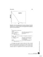
7.9 Application of the dyadic wavelet transform to nonlinear filtering.
After subband decomposition using an analysis filter bank, a threshold process is
applied to the two highest resolution highpass subbands before reconstruction
using a synthesis filter bank. Periodic convolution was used so that there is no
phase shift between the input and output signals.
an = analyze1(x,h0,4); % Decompose signal, analytic
% filter bank of level 4
% Set the threshold times to equal the variance of the two higher
% resolution highpass subbands.
threshold = var(an(N/4:N));
for i = (N/4:N) % Examine the two highest
% resolution highpass
% subbands
if an(i) < threshold
an(i) = 0;
end
end
sy = synthesize1(an,h0,4); % Reconstruct original
% signal
figure(fig2);
plot(t,x,’k’,t,sy-5,’k’); % Plot signals
axis([ 2 1.2-8 4]); xlabel(’Time(sec)’)
TLFeBOOK
202 Chapter 7
The routines for the analysis and synthesis filter banks differ slightly from
those used in Example 7.3 in that they use circular convolution. In the analysis
filter bank routine (
analysis1

), the data are first extended using the periodic
or wraparound approach: the initial points are added to the end of the original
data sequence (see Figure 2.10B). This extension is the same length as the
filter. After convolution, these added points and the extra points generated by
convolution are removed in a symmetrical fashion: a number of points equal to
the filter length are removed from the initial portion of the output and the re-
maining extra points are taken off the end. Only the code that is different from
that shown in Example 7.3 is shown below. In this code, symmetric elimination
of the additional points and downsampling are done in the same instruction.
function an = analyze1(x,h0,L)

for i = 1:L
a_ext = [an an(1:lf)]; % Extend data for “periodic
% convolution”
lpf = conv(a_ext,h0); % Lowpass FIR filter
hpf = conv(a_ext,h1); % Highpass FIR filter
lpfd = lpf(lf:2:lf؉lx-1); % Remove extra points. Shift to
hpfd = hpf(lf:2:lf؉lx-1); % obtain circular segment; then
% downsample
an(1:lx) = [lpfd hpfd]; % Lowpass output at beginning of
% array, but now occupies only
% half the data points as last
% pass
lx = lx/2;
The synthesis filter bank routine is modified in a similar fashion except
that the initial portion of the data is extended, also in wraparound fashion (by
adding the end points to the beginning). The extended segments are then upsam-
pled, convolved with the filters, and added together. The extra points are then
removed in the same manner used in the analysis routine. Again, only the modi-
fied code is shown below.

function y = synthesize1(an,h0,L)

for i = 1:L
lpx = y(1:lseg); % Get lowpass segment
hpx = y(lseg؉1:2*lseg); % Get highpass outputs
lpx = [lpx(lseg-lf/2؉1:lseg) lpx]; % Circular extension:
% lowpass comp.
hpx = [hpx(lseg-lf/2؉1:lseg) hpx]; % and highpass component
l_ext = length(lpx);
TLFeBOOK
Wavelet Analysis 203
up_lpx = zeros(1,2*l_ext); % Initialize vector for
% upsampling
up_lpx(1:2:2*l_ext) = lpx; % Up sample lowpass (every
% odd point)
up_hpx = zeros(1,2*l_ext); % Repeat for highpass
up_hpx(1:2:2*l_ext) = hpx;
syn = conv(up_lpx,g0) ؉ conv(up_hpx,g1); % Filter and
% combine
y(1:2*lseg) = syn(lf؉1:(2*lseg)؉lf); % Remove extra
% points
lseg = lseg * 2; % Double segment lengths
% for next pass
end

The original and reconstructed waveforms are shown in Figure 7.9. The
filtering produced by thresholding the highpass subbands is evident. Also there
is no phase shift between the original and reconstructed signal due to the use of
periodic convolution, although a small artifact is seen at the beginning and end
of the data set. This is because the data set was not really periodic.

Discontinuity Detection
Wavelet analysis based on filter bank decomposition is particularly useful for
detecting small discontinuities in a waveform. This feature is also useful in
image processing. Example 7.5 shows the sensitivity of this method for detect-
ing small changes, even when they are in the higher derivatives.
Example 7.5 Construct a waveform consisting of 2 sinusoids, then add
a small (approximately 1% of the amplitude) offset to this waveform. Create a
new waveform by double integrating the waveform so that the offset is in the
second derivative of this new signal. Apply a three-level analysis filter bank.
Examine the high frequency subband for evidence of the discontinuity.
% Example 7.5 and Figures 7.10 and 7.11. Discontinuity detection
% Construct a waveform of 2 sinusoids with a discontinuity
% in the second derivative
% Decompose the waveform into 3 levels to detect the
% discontinuity.
% Use Daubechies 4-element filter
%
close all; clear all;
fig1 = figure(’Units’,’inches’,’Position’,[0 2.5 3 3.5]);
fig2 = figure(’Units’, ’inches’,’Position’,[3 2.5 5 5]);
fs = 1000; % Sample frequency
TLFeBOOK
204 Chapter 7
F
IGURE
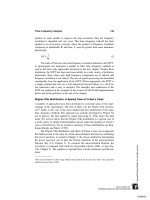
7.10 Waveform composed of two sine waves with an offset discontinuity
in its second derivative at 0.5 sec. Note that the discontinuity is not apparent in
the waveform.
N = 1024; % Number of points in
% waveform

freqsin = [.23 .8 1.8]; % Sinusoidal frequencies
ampl = [1.2 1 .7]; % Amplitude of sinusoid
incr = .01; % Size of second derivative
% discontinuity
offset = [zeros(1,N/2) ones(1,N/2)];
h0 = daub(4) % Daubechies 4
%
[x1 t] = signal(freqsin,ampl,N); % Construct signal
x1 = x1 ؉ offset*incr; % Add discontinuity at
% midpoint
x = integrate(integrate(x1)); % Double integrate
figure(fig1);
plot(t,x,’k’,t,offset-2.2,’k’); % Plot new signal
axis([0 1-2.5 2.5]);
xlabel(’Time (sec)’);
TLFeBOOK
Wavelet Analysis 205
F
IGURE
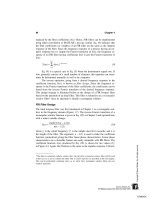
7.11 Analysis filter bank output of the signal shown in Figure 7.10. Al-
though the discontinuity is not visible in the original signal, its presence and loca-
tion are clearly identified as a spike in the highpass subbands.
TLFeBOOK
206 Chapter 7
figure(fig2);
a = analyze(x,h0,3); % Decompose signal, analytic
% filter bank of level 3
Figure 7.10 shows the waveform with a discontinuity in its second deriva-
tive at 0.5 sec. The lower trace indicates the position of the discontinuity. Note
that the discontinuity is not visible in the waveform.

The output of the three-level analysis filter bank using the Daubechies 4-
element filter is shown in Figure 7.11. The position of the discontinuity is
clearly visible as a spike in the highpass subbands.
Feature Detection: Wavelet Packets
The DWT can also be used to construct useful descriptors of a waveform. Since
the DWT is a bilateral transform, all of the information in the original waveform
must be contained in the subband signals. These subband signals, or some aspect
of the subband signals such as their energy over a given time period, could
provide a succinct description of some important aspect of the original signal.
In the decompositions described above, only the lowpass filter subband
signals were sent on for further decomposition, giving rise to the filter bank
structure shown in the upper half of Figure 7.12. This decomposition structure
is also known as a logarithmic tree. However, other decomposition structures
are valid, including the complete or balanced tree structure shown in the lower
half of Figure 7.12. In this decomposition scheme, both highpass and lowpass
subbands are further decomposed into highpass and lowpass subbands up till
the terminal signals. Other, more general, tree structures are possible where a
decision on further decomposition (whether or not to split a subband signal)
depends on the activity of a given subband. The scaling functions and wavelets
associated with such general tree structures are known as wavelet packets.
Example 7.6 Apply balanced tree decomposition to the waveform con-
sisting of a mixture of three equal amplitude sinusoids of 1 10 and 100 Hz. The
main routine in this example is similar to that used in Examples 7.3 and 7.4
except that it calls the balanced tree decomposition routine,
w_packet
, and plots
out the terminal waveforms. The
w_packet
routine is shown below and is used
in this example to implement a 3-level decomposition, as illustrated in the lower

half of Figure 7.12. This will lead to 8 output segments that are stored sequen-
tially in the output vector,
a
.
% Example 7.5 and Figure 7.13
% Example of “Balanced Tree Decomposition”
% Construct a waveform of 4 sinusoids plus noise
% Decompose the waveform in 3 levels, plot outputs at the terminal
% level
TLFeBOOK
Wavelet Analysis 207
F
IGURE
7.12 Structure of the analysis filter bank (wavelet tree) used in the DWT
in which only the lowpass subbands are further decomposed and a more general
structure in which all nonterminal signals are decomposed into highpass and low-
pass subbands.
% Use a Daubechies 10 element filter
%
clear all; close all;
fig1 = figure(’Units’,’inches’,’Position’,[0 2.5 3 3.5]);
fig2 = figure(’Units’, ’inches’,’Position’,[3 2.5 5 4]);
fs = 1000; % Sample frequency
N = 1024; % Number of points in
% waveform
levels = 3 % Number of decomposition
% levels
nu_seg = 2vlevels; % Number of decomposed
% segments
freqsin = [1 10 100]; % Sinusoid frequencies

TLFeBOOK
208 Chapter 7
F
IGURE
7.13 Balanced tree decomposition of the waveform shown in Figure 7.8.
The signal from the upper left plot has been lowpass filtered 3 times and repre-
sents the lowest terminal signal in Figure 7.11. The upper right has been lowpass
filtered twice then highpass filtered, and represents the second from the lowest
terminal signal in Figure 7.11. The rest of the plots follow sequentially.
TLFeBOOK
Wavelet Analysis 209
ampl = [1 1 1]; % Amplitude of sinusoid
h0 = daub(10); % Get filter coefficients:
% Daubechies 10
%
[x t] = signal(freqsin,ampl,N); % Construct signal
a = w_packet(x,h0,levels); % Decompose signal, Balanced
% Tree
for i = 1:nu_seg
i_s = 1 ؉ (N/nu_seg) * (i-1); % Location for this segment
a_p = a(i_s:i_s؉(N/nu_seg)-1);
subplot(nu_seg/2,2,i); % Plot decompositions
plot((1:N/nu_seg),a_p,’k’);
xlabel(’Time (sec)’);
end
The balanced tree decomposition routine,
w_packet
, operates similarly to
the DWT analysis filter banks, except for the filter structure. At each level,
signals from the previous level are isolated, filtered (using standard convolu-

tion), downsampled, and both the high- and lowpass signals overwrite the single
signal from the previous level. At the first level, the input waveform is replaced
by the filtered, downsampled high- and lowpass signals. At the second level,
the two high- and lowpass signals are each replaced by filtered, downsampled
high- and lowpass signals. After the second level there are now four sequential
signals in the original data array, and after the third level there be will be eight.
% Function to generate a “balanced tree” filter bank
% All arguments are the same as in routine ‘analyze’
%an = w_packet(x,h,L)
% where
%x= input waveform (must be longer than 2vL ؉ L and power of
% two)
%h0= filter coefficients (low pass)
%L= decomposition level (number of High pass filter in bank)
%
function an = w_packet(x,h0,L)
lf = length(h0); % Filter length
lx = length(x); % Data length
an = x; % Initialize output
% Calculate High pass coefficients from low pass coefficients
for i = 0:(lf-1)
h1(i؉1) = (-1)vi * h0(lf-i); % Uses Eq. (18)
end
% Calculate filter outputs for all levels
for i = 1:L
TLFeBOOK
210 Chapter 7
nu_low = 2v(i-1); % Number of lowpass filters
% at this level
l_seg = lx/2v(i-1); % Length of each data seg. at

% this level
for j = 1:nu_low;
i_start = 1 ؉ l_seg * (j-1); % Location for current
% segment
a_seg = an(i_start:i_start؉l_seg-1);
lpf = conv(a_seg,h0); % Lowpass filter
hpf = conv(a_seg,h1); % Highpass filter
lpf = lpf(1:2:l_seg); % Downsample
hpf = hpf(1:2:l_seg);
an(i_start:i_start؉l_seg-1) = [lpf hpf];
end
end
The output produced by this decomposition is shown in Figure 7.13. The
filter bank outputs emphasize various components of the three-sine mixture.
Another example is given in Problem 7 using a chirp signal.
One of the most popular applications of the dyadic wavelet transform is
in data compression, particularly of images. However, since this application is
not so often used in biomedical engineering (although there are some applica-
tions regrading the transmission of radiographic images), it will not be covered
here.
PROBLEMS
1. (A) Plot the frequency characteristics (magnitude and phase) of the Mexi-
can hat and Morlet wavelets.
(B) The plot of the phase characteristics will be incorrect due to phase wrapping.
Phase wrapping is due to the fact that the arctan function can never be greater
that ± 2π; hence, once the phase shift exceeds ± 2π (usually minus), it warps
around and appears as positive. Replot the phase after correcting for this wrap-
around effect. (Hint: Check for discontinuities above a certain amount, and
when that amount is exceeded, subtract 2π from the rest of the data array. This
is a simple algorithm that is generally satisfactory in linear systems analysis.)

2. Apply the continuous wavelet analysis used in Example 7.1 to analyze a
chirp signal running between 2 and 30 Hz over a 2 sec period. Assume a sample
rate of 500 Hz as in Example 7.1. Use the Mexican hat wavelet. Show both
contour and 3-D plot.
3. Plot the frequency characteristics (magnitude and phase) of the Haar and
Daubechies 4-and 10-element filters. Assume a sample frequency of 100 Hz.
TLFeBOOK
Wavelet Analysis 211
4. Generate a Daubechies 10-element filter and plot the magnitude spectrum
as in Problem 3. Construct the highpass filter using the alternating flip algorithm
(Eq. (20)) and plot its magnitude spectrum. Generate the lowpass and highpass
synthesis filter coefficients using the order flip algorithm (Eqs. (23) and (24))
and plot their respective frequency characteristics. Assume a sampling fre-
quency of 100 Hz.
5. Construct a waveform of a chirp signal as in Problem 2 plus noise. Make
the variance of the noise equal to the variance of the chirp. Decompose the
waveform in 5 levels, operate on the lowest level (i.e., the high resolution high-
pass signal), then reconstruct. The operation should zero all elements below a
given threshold. Find the best threshold. Plot the signal before and after recon-
struction. Use Daubechies 6-element filter.
6. Discontinuity detection. Load the waveform
x
in file
Prob7_6_data
which
consists of a waveform of 2 sinusoids the same as in Figure 7.9, but with a
series of diminishing discontinuities in the second derivative. The discontinuities
in the second derivative begin at approximately 0.5% of the sinusoidal ampli-
tude and decrease by a factor of 2 for each pair of discontinuities. (The offset
array can be obtained in the variable

offset
.) Decompose the waveform into
three levels and examine and plot only the highest resolution highpass filter
output to detect the discontinuity. Hint : The highest resolution output will be
located in N/2 to N of the
analysis
output array. Use a Harr and a Daubechies
10-element filter and compare the difference in detectability. (Note that the Haar
is a very weak filter so that some of the low frequency components will still be
found in its output.)
7. Apply the balanced tree decomposition to a chirp signal similar to that used
in Problem 5 except that the chirp frequency should range between 2 and 100
Hz. Decompose the waveform into 3 levels and plot the outputs at the terminal
level as in Example 7.5. Use a Daubechies 4-element filter. Note that each
output filter responds to different portions of the chirp signal.
TLFeBOOK
TLFeBOOK
8
Advanced Signal Processing
Techniques: Optimal
and Adaptive Filters
OPTIMAL SIGNAL PROCESSING: WIENER FILTERS
The FIR and IIR filters described in Chapter 4 provide considerable flexibility
in altering the frequency content of a signal. Coupled with MATLAB filter
design tools, these filters can provide almost any desired frequency characteris-
tic to nearly any degree of accuracy. The actual frequency characteristics at-
tained by the various design routines can be verified through Fourier transform
analysis. However, these design routines do not tell the user what frequency
characteristics are best; i.e., what type of filtering will most effectively separate
out signal from noise. That decision is often made based on the user’s knowl-

edge of signal or source properties, or by trial and error. Optimal filter theory
was developed to provide structure to the process of selecting the most appro-
priate frequency characteristics.
A wide range of different approaches can be used to develop an optimal
filter, depending on the nature of the problem: specifically, what, and how
much, is known about signal and noise features. If a representation of the de-
sired signal is available, then a well-developed and popular class of filters
known as Wiener filters can be applied. The basic concept behind Wiener filter
theory is to minimize the difference between the filtered output and some de-
sired output. This minimization is based on the least mean square approach,
which adjusts the filter coefficients to reduce the square of the difference be-
tween the desired and actual waveform after filtering. This approach requires
213
TLFeBOOK
214 Chapter 8
F
IGURE
8.1 Basic arrangement of signals and processes in a Wiener filter.
an estimate of the desired signal which must somehow be constructed, and this
estimation is usually the most challenging aspect of the problem.*
The Wiener filter approach is outlined in Figure 8.1. The input waveform
containing both signal and noise is operated on by a linear process, H(z). In
practice, the process could be either an FIR or IIR filter; however, FIR filters
are more popular as they are inherently stable,† and our discussion will be
limited to the use of FIR filters. FIR filters have only numerator terms in the
transfer function (i.e., only zeros) and can be implemented using convolution
first presented in Chapter 2 (Eq. (15)), and later used with FIR filters in Chapter
4 (Eq. (8)). Again, the convolution equation is:
y(n) =
∑

L
k=1
b(k) x(n − k)(1)
where h(k) is the impulse response of the linear filter. The output of the filter,
y(n), can be thought of as an estimate of the desired signal, d(n). The difference
between the estimate and desired signal, e(n), can be determined by simple
subtraction: e(n) = d(n) − y(n).
As mentioned above, the least mean square algorithm is used to minimize
the error signal: e(n) = d(n) − y(n). Note that y(n) is the output of the linear
filter, H(z). Since we are limiting our analysis to FIR filters, h(k) ≡ b(k), and
e(n) can be written as:
e(n) = d(n) − y(n) = d(n) −
∑
L−1
k=0
h(k) x(n − k)(2)
where L is the length of the FIR filter. In fact, it is the sum of e(n)
2
which is
minimized, specifically:
*As shown below, only the crosscorrelation between the unfiltered and the desired output is neces-
sary for the application of these filters.
†IIR filters contain internal feedback paths and can oscillate with certain parameter combinations.
TLFeBOOK
Advanced Signal Processing 215
ε=
∑
N
n=1
e

2
(n) =
∑
N
n=1
ͫ
d(n) −
∑
L
k=1
b(k) x(n − k)
ͬ
2
(3)
After squaring the term in brackets, the sum of error squared becomes a
quadratic function of the FIR filter coefficients, b(k), in which two of the terms
can be identified as the autocorrelation and cross correlation:
ε=
∑
N
n=1
d(n) − 2
∑
L
k=1
b(k)r
dx
(k) +
∑
L

k=1
∑
L
R=1
b(k) b(R)r
xx
(k − R) (4)
where, from the original definition of cross- and autocorrelation (Eq. (3), Chap-
ter 2):
r
dx
(k) =
∑
L
R=1
d(R) x(R + k)
r
xx
(k) =
∑
L
R=1
x(R) x(R + k)
Since we desire to minimize the error function with respect to the FIR
filter coefficients, we take derivatives with respect to b(k) and set them to zero:
∂ε
∂b(k)
= 0; which leads to:
∑
L

k=1
b(k) r
xx
(k − m) = r
dx
(m), for 1 ≤ m ≤ L (5)
Equation (5) shows that the optimal filter can be derived knowing only
the autocorrelation function of the input and the crosscorrelation function be-
tween the input and desired waveform. In principle, the actual functions are
not necessary, only the auto- and crosscorrelations; however, in most practical
situations the auto- and crosscorrelations are derived from the actual signals, in
which case some representation of the desired signal is required.
To solve for the FIR coefficients in Eq. (5), we note that this equation
actually represents a series of L equations that must be solved simultaneously.
The matrix expression for these simultaneous equations is:
ͫ
r
xx
(0) r
xx
(1)

r
xx
(L)
r
xx
(1) r
xx
(0)

r
xx
(L − 1)
ӇӇO Ӈ
r
xx
(L) r
xx
(L − 1)

r
xx
(0)
ͬͫ
b(0)
b(1)
Ӈ
b(L)
ͬ
=
ͫ
r
dx
(0)
r
dx
(1)
Ӈ
r

dx
(L)
ͬ
(6)
Equation (6) is commonly known as the Wiener-Hopf equation and is a
basic component of Wiener filter theory. Note that the matrix in the equation is
TLFeBOOK
216 Chapter 8
F
IGURE
8.2 Configuration for using optimal filter theory for systems identification.
the correlation matrix mentioned in Chapter 2 (Eq. (21)) and has a symmetrical
structure termed a Toeplitz structure.* The equation can be written more suc-
cinctly using standard matrix notation, and the FIR coefficients can be obtained
by solving the equation through matrix inversion:
RB = r
dx
and the solution is: b = R
−1
r
dx
(7)
The application and solution of this equation are given for two different
examples in the following section on MATLAB implementation.
The Wiener-Hopf approach has a number of other applications in addition
to standard filtering including systems identification, interference canceling, and
inverse modeling or deconvolution. For system identification, the filter is placed
in parallel with the unknown system as shown in Figure 8.2. In this application,
the desired output is the output of the unknown system, and the filter coeffi-
cients are adjusted so that the filter’s output best matches that of the unknown

system. An example of this application is given in a subsequent section on
adaptive signal processing where the least mean squared (LMS) algorithm is
used to implement the optimal filter. Problem 2 also demonstrates this approach.
In interference canceling, the desired signal contains both signal and noise while
the filter input is a reference signal that contains only noise or a signal correlated
with the noise. This application is also explored under the section on adaptive
signal processing since it is more commonly implemented in this context.
MATLAB Implementation
The Wiener-Hopf equation (Eqs. (5) and (6 ), can be solved using MATLAB’s
matrix inversion operator (‘\’) as shown in the examples below. Alternatively,
*Due to this matrix’s symmetry, it can be uniquely defined by only a single row or column.
TLFeBOOK
Advanced Signal Processing 217
since the matrix has the Toeplitz structure, matrix inversion can also be done
using a faster algorithm known as the Levinson-Durbin recursion.
The MATLAB
toeplitz
function is useful in setting up the correlation
matrix. The function call is:
Rxx = toeplitz(rxx);
where
rxx
is the input row vector. This constructs a symmetrical matrix from a
single row vector and can be used to generate the correlation matrix in Eq. (6)
from the autocorrelation function r
xx
. (The function can also create an asymmet-
rical Toeplitz matrix if two input arguments are given.)
In order for the matrix to be inverted, it must be nonsingular; that is, the
rows and columns must be independent. Because of the structure of the correla-

tion matrix in Eq. (6) (termed positive- definite), it cannot be singular. However,
it can be near singular: some rows or columns may be only slightly independent.
Such an ill-conditioned matrix will lead to large errors when it is inverted. The
MATLAB ‘\’ matrix inversion operator provides an error message if the matrix
is not well-conditioned, but this can be more effectively evaluated using the
MATLAB
cond
function:
c = cond(X)
where
X
is the matrix under test and
c
is the ratio of the largest to smallest
singular values. A very well-conditioned matrix would have singular values in
the same general range, so the output variable,
c
, would be close to one. Very
large values of
c
indicate an ill-conditioned matrix. Values greater than 10
4
have
been suggested by Sterns and David (1996) as too large to produce reliable
results in the Wiene r-Hopf equation. When thi s occurs, the cond iti on of the matri x
can usually be improved by reducing its dimension, that is, reducing the range,
L, of the autocorrelation function in Eq (6). This will also reduce the number
of filter coefficients in the solution.
Example 8.1 Given a sinusoidal signal in noise (SNR = -8 db), design
an optimal filter using the Wiener-Hopf equation. Assume that you have a copy

of the actual signal available, in other words, a version of the signal without the
added noise. In general, this would not be the case: if you had the desired signal,
you would not need the filter! In practical situations you would have to estimate
the desired signal or the crosscorrelation between the estimated and desired
signals.
Solution The program below uses the routine
wiener_hopf
(also shown
below) to determine the optimal filter coefficients. These are then applied to the
noisy waveform using the
filter
routine introduced in Chapter 4 although
correlation could also have been used.
TLFeBOOK
218 Chapter 8
% Example 8.1 and Figure 8.3 Wiener Filter Theory
% Use an adaptive filter to eliminate broadband noise from a
% narrowband signal
% Implemented using Wiener-Hopf equations
%
close all; clear all;
fs = 1000; % Sampling frequency
F
IGURE
8.3 Applicatio n of the Wiener-Hopf equation to produce an optimal FIR
filter to filter broa dban d noise (SNR = -8 db ) from a single sinusoi d (10 Hz.) The
frequency character isti cs (bottom plot) show that the filter coefficients were adjusted
to approxim ate a bandpass filter w ith a small bandwidth an d a p eak a t 10 H z.
TLFeBOOK
Advanced Signal Processing 219

N = 1024; % Number of points
L = 256; % Optimal filter order
%
% Generate signal and noise data: 10 Hz sin in 8 db noise (SNR =
%-8db)
[xn, t, x] = sig_noise(10,-8,N); % xn is signal ؉ noise and
% x is noise free (i.e.,
% desired) signal
subplot(3,1,1); plot(t, xn,’k’); % Plot unfiltered data
labels, table, axis
%
% Determine the optimal FIR filter coefficients and apply
b = wiener_hopf(xn,x,L); % Apply Wiener-Hopf
% equations
y = filter(b,1,xn); % Filter data using optimum
% filter weights
%
% Plot filtered data and filter spectrum
subplot(3,1,2); plot(t,y,’k’); % Plot filtered data
labels, table, axis
%
subplot(3,1,3);
f = (1:N) * fs/N; % Construct freq. vector for plotting
h = abs(fft(b,256)).v2 % Calculate filter power
plot(f,h,’k’); % spectrum and plot
labels, table, axis
The function
Wiener_hopf
solves the Wiener-Hopf equations:
function b = wiener_hopf(x,y,maxlags)

% Function to compute LMS algol using Wiener-Hopf equations
% Inputs: x = input
%y= desired signal
% Maxlags = filter length
% Outputs: b = FIR filter coefficients
%
rxx = xcorr(x,maxlags,’coeff’); % Compute the autocorrela-
% tion vector
rxx = rxx(maxlags؉1:end)’; % Use only positive half of
% symm. vector
rxy = xcorr(x,y,maxlags); % Compute the crosscorrela-
% tion vector
rxy = rxy(maxlags؉1:end)’; % Use only positive half
%
rxx_matrix = toeplitz(rxx); % Construct correlation
% matrix
TLFeBOOK
220 Chapter 8
b = rxx_matrix(rxy; % Calculate FIR coefficients
% using matrix inversion,
% Levinson could be used
% here
Example 8.1 generates Figure 8.3 above. Note that the optimal filter ap-
proach, when applied to a single sinusoid buried in noise, produces a bandpass
filter with a peak at the sinusoidal frequency. An equivalent—or even more
effective—filter could have been designed using the tools presented in Chapter
4. Indeed, such a statement could also be made about any of the adaptive filters
described below. However, this requires precise a priori knowledge of the signal
and noise frequency characteristics, which may not be available. Moreover, a
fixed filter will not be able to optimally filter signal and noise that changes over

time.
Example 8.2 Apply the LMS algorithm to a systems identification task.
The “unknown” system will be an all-zero linear process with a digital transfer
function of:
H(z) = 0.5 + 0.75z
−1
+ 1.2z
−2
Confirm the match by plotting the magnitude of the transfer function for
both the unknown and matching systems. Since this approach uses an FIR filter
as the matching system, which is also an all -zero process, the match should be
quite good. In Problem 2, this approach is repeated, but for an unknown system
that has both poles and zeros. In this case, the FIR (all-zero) filter will need
many more coefficients than the unknown pole-zero process to produce a rea-
sonable match.
Solution The program below inputs random noise into the unknown pro-
cess using convolution and into the matching filter. Since the FIR matching
filter cannot easily accommodate for a pure time delay, care must be taken to
compensate for possible time shift due to the convolution operation. The match-
ing filter coefficients are adjusted using the Wiener-Hopf equation described
previously. Frequency characteristics of both unknown and matching system are
determined by applying the FFT to the coefficients of both processes and the
resultant spectra are plotted.
% Example 8.2 and Figure 8.4 Adaptive Filters System
% Identification
%
% Uses optimal filtering implemented with the Wiener-Hopf
% algorithm to identify an unknown system
%
% Initialize parameters

TLFeBOOK
Advanced Signal Processing 221
F
IGURE
8.4 Frequency characteristics of an “unknown” process having coeffi-
cients of 0.5, 0.75, and 1.2 (an all-zero process). The matching process uses
system identification implemented with the Wiener-Hopf adaptive filtering ap-
proach. This matching process generates a linear system with a similar spectrum
to the unknown process. Since the unknown process is also an all-zero system,
the transfer function coefficients also match.
close all; clear all;
fs = 500; % Sampling frequency
N = 1024; % Number of points
L = 8; % Optimal filter order
%
% Generate unknown system and noise input
b_unknown = [.5 .75 1.2]; % Define unknown process
xn = randn(1,N);
xd = conv(b_unknown,xn); % Generate unknown system output
xd = xd(3:N؉2); % Truncate extra points.
% Ensure proper phase
% Apply Weiner filter
b = wiener_hopf(xn,xd,L); % Compute matching filter
% coefficients
b = b/N; % Scale filter coefficients
%
% Calculate frequency characteristics using the FFT
ps_match = (abs(fft(b,N))).v2;
ps_unknown = (abs(fft(b_unknown,N))).v2;
TLFeBOOK

222 Chapter 8
%
% Plot frequency characteristics of unknown and identified
% process
f = (1:N) * fs/N; % Construct freq. vector for
% plotting
subplot(1,2,1); % Plot unknown system freq. char.
plot(f(1:N/2),ps_unknown(1:N/2),’k’);
labels, table, axis
subplot(1,2,2);
% Plot matching system freq. char.
plot(f(1:N/2),ps_match(1:N/2),’k’);
labels, table, axis
The output plots from this example are shown in Figure 8.4. Note the
close match in spectral characteristics between the “unknown” process and the
matching output produced by the Wiener-Hopf algorithm. The transfer functions
also closely match as seen by the similarity in impulse response coefficients:
h(n)
unknown
= [0.5 0.75 1.2]; h(n)
match
= [0.503 0.757 1.216].
ADAPTIVE SIGNAL PROCESSING
The area of adaptive signal processing is relatively new yet already has a rich
history. As with optimal filtering, only a brief example of the usefulness and
broad applicability of adaptive filtering can be covered here. The FIR and IIR
filters described in Chapter 4 were based on an a priori design criteria and were
fixed throughout their application. Although the Wiener filter described above
does not require prior knowledge of the input signal (only the desired outcome),
it too is fixed for a given application. As with classical spectral analysis meth-

ods, these filters cannot respond to changes that might occur during the course
of the signal. Adaptive filters have the capability of modifying their properties
based on selected features of signal being analyzed.
A typical adaptive fi lter paradigm is shown in Figu re 8.5 . In this cas e, the
filter co effic ients are modified by a feedback pro cess designed to make the filter’s
output, y(n), as close to some desired response, d(n), as possible, by reducing the
error, e(n), to a minimum. As with optimal filtering, the nature of the desi red
response will depend on the specific problem involved and its formulation may
be the most diff icult part o f the a dapti ve sys tem sp ecification (Stearns and David,
1996).
The inherent stabili ty of FIR fil ters makes t hem attract ive in adapt ive ap pli-
cations as well as in optimal filtering (Ingle and Proakis, 2000). Accordingly, the
adaptive filte r, H(z), can again be represented by a set of FIR f ilter coefficients,
TLFeBOOK
Advanced Signal Processing 223
F
IGURE
8.5 Elements of a typical adaptive filter.
b(k). The FIR filter equati on (i.e., convolution) is repeated here, but the filter
coefficients are indicated as b
n
(k) to ind icate that they vary with time (i.e., n).
y(n) =
∑
L
k=1
b
n
(k) x(n − k)(8)
The adaptive filter operates by modifying the filter coefficients, b

n
(k),
based on some signal property. The general adaptive filter problem has similari-
ties to the Wiener filter theory problem discussed above in that an error is
minimized, usually between the input and some desired response. As with opti-
mal filtering, it is the squared error that is minimized, and, again, it is necessary
to somehow construct a desired signal. In the Wiener approach, the analysis is
applied to the entire waveform and the resultant optimal filter coefficients were
similarly applied to the entire waveform (a so-called block approach). In adap-
tive filtering, the filter coefficients are adjusted and applied in an ongoing basis.
While the Wiener-Hopf equ at ion s (Eqs. (6) and (7)) can be, and have been,
adapted for use in an adaptive environment, a simpler and more popular ap-
proach is based on gradient optimization. This approach is usually called the
LMS recursive algorithm. As in Wiener filter theory, this algorithm also deter-
mines the optimal filter coefficients, and it is also based on minimizing the
squared error, but it does not require computation of the correlation functions,
r
xx
and r
xy
. Instead the LMS algorithm uses a recursive gradient method known
as the steepest-descent method for finding the filter coefficients that produce
the minimum sum of squared error.
Examination of Eq. (3) shows that the sum of squared errors is a quadratic
function of the FIR filter coefficients, b(k); hence, this function will have a
single minimum. The goal of the LMS algorithm is to adjust the coefficients so
that the sum of squared error moves toward this minimum. The technique used
by the LMS algorithm is to adjust the filter coefficients based on the method of
steepest descent. In this approach, the filter coefficients are modified based on
TLFeBOOK

224 Chapter 8
an estimate of the negative gradient of the error function with respect to a given
b(k). This estimate is given by the partial derivative of the squared error, ε, with
respect to the coefficients, b
n
(k):
᭞
n
=
∂ε
n
2
∂b
n
(k)
= 2e(n)
∂(d(n) − y(n))
∂b
n
(k)
(9)
Since d(n) is independent of the coefficients, b
n
(k), its partial derivative
with respect to b
n
(k) is zero. As y(n) is a function of the input times b
n
(k) (Eq.
(8)), then its partial derivative with respect to b

n
(k) is just x(n-k), and Eq. (9)
can be rewritten in terms of the instantaneous product of error and the input:
᭞
n
= 2e(n) x(n − k)(10)
Initially, the filter coefficients are set arbitrarily to some b
0
(k), usually
zero. With each new input sample a new error signal, e(n), can be computed
(Figure 8.5). Based on this new error signal, the new gradient is determined
(Eq. (10)), and the filter coefficients are updated:
b
n
(k) = b
n−1
(k) +∆e(n) x(n − k)(11)
where ∆ is a constant that controls the descent and, hence, the rate of conver-
gence. This parameter must be chosen with some care. A large value of ∆ will
lead to large modifications of the filter coefficients which will hasten conver-
gence, but can also lead to instability and oscillations. Conversely, a small value
will result in slow convergence of the filter coefficients to their optimal values.
A common rule is to select the convergence parameter, ∆, such that it lies in
the range:
0 <∆<
1
10LP
x
(12)
where L is the length of the FIR filter and P

x
is the power in the input signal.
P
X
can be approximated by:
P
x
Ϸ
1
N − 1
∑
N
n=1
x
2
(n)(13)
Note that for a waveform of zero mean, P
x
equals the variance of x. The
LMS algorithm given in Eq. (11) can easily be implemented in MATLAB, as
shown in the next section.
Adaptive filtering has a number of applications in biosignal processing. It
can be used to suppress a narrowband noise source such as 60 Hz that is corrupt-
ing a broadband signal. It can also be used in the reverse situation, removing
broadband noise from a narrowband signal, a process known as adaptive line
TLFeBOOK
Advanced Signal Processing 225
F
IGURE
8.6 Configuration for Adaptive Line Enhancement (ALE) or Adaptive In-

terference Suppression. The Delay, D, decorrelates the narrowband component
allowing the adaptive filter to use only this component. In ALE the narrowband
component is the signal while in Interference suppression it is the noise.
enhancement (ALE).* It can also be used for some of the same applications
as the Wiener filter such as system identification, inverse modeling, and, espe-
cially important in biosignal processing, adaptive noise cancellation. This last
application requires a suitable reference source that is correlated with the noise,
but not the signal. Many of these applications are explored in the next section
on MATLAB implementation and/or in the problems.
The configuration for ALE and adaptive interference suppression is shown
in Figure 8.6. When this configuration is used in adaptive interference suppres-
sion, the input consists of a broadband signal, Bb(n), in narrowband noise,
Nb(n), such as 60 Hz. Since the noise is narrowband compared to the relatively
broadband signal, the noise portion of sequential samples will remain correlated
while the broadband signal components will be decorrelated after a few sam-
ples.† If the combined signal and noise is delayed by D samples, the broadband
(signal) component of the delayed waveform will no longer be correlated with
the broadband component in the original waveform. Hence, when the filter’s
output is subtracted from the input waveform, only the narrowband component
*The adaptive line enhancer is so termed because the objective of this filter is to enhance a narrow-
band signal, one with a spectrum composed of a single “line.”
†Recall that the width of the autocorrelation function is a measure of the range of samples for which
the samples are correlated, and this width is inversely related to the signal bandwidth. Hence, broad-
band signals remain correlated for only a few samples and vice versa.
TLFeBOOK