Beginning Databases with Postgre SQL phần 4 pptx

CHAPTER 7 ■ ADVANCED DATA SELECTION
175
■Note In the examples in this chapter, as with others, we start with clean base data in the sample data-
base, so readers can dip into chapters as they choose. This does mean that some of the output will be slightly
different if you continue to use sample data from a previous chapter. The downloadable code for this book
(available from the Downloads section of the Apress web site at ) provides scripts
to make it easy to drop the tables, re-create them, and repopulate them with clean data, if you wish to do so.
Try It Out: Use Count(*)
Suppose we wanted to know how many customers in the customer table live in the town of
Bingham. We could simply write a SQL query like this:
SELECT * FROM customer WHERE town = 'Bingham';
Or, for a more efficient version that returns less data, we could write a SQL query like this:
SELECT customer_id FROM customer WHERE town = 'Bingham';
This works, but in a rather indirect way. Suppose the customer table contained many
thousands of customers, with perhaps over a thousand of them living in Bingham. In that case,
we would be retrieving a great deal of data that we don’t need. The count(*) function solves
this for us, by allowing us to retrieve just a single row with the count of the number of selected
rows in it.
We write our SELECT statement as we normally do, but instead of selecting real columns,
we use count(*), like this:
bpsimple=# SELECT count(*) FROM customer WHERE town = 'Bingham';
count

3
(1 row)
bpsimple=#
If we want to count all the customers, we can just omit the WHERE clause:
bpsimple=# SELECT count(*) FROM customer;
count

15

(1 row)
bpsimple=#
You can see we get just a single row, with the count in it. If you want to check the answer,
just replace count(*) with customer_id to show the real data.
MatthewStones_4789C07.fm Page 175 Tuesday, February 1, 2005 7:33 AM
176
CHAPTER 7
■ ADVANCED DATA SELECTION
How It Works
The count(*) function allows us to retrieve a count of objects, rather than the objects them-
selves. It is vastly more efficient than getting the data itself, because all of the data that we don’t
need to see does not need to be retrieved from the database, or worse still, sent across a network.
■Tip You should never retrieve data when all you need is a count of the number of rows.
GROUP BY and Count(*)
Suppose we wanted to know how many customers live in each town. We could find out by
selecting all the distinct towns, and then counting how many customers were in each town.
This is a rather procedural and tedious way of solving the problem. Wouldn’t it be better to
have a declarative way of simply expressing the question directly in SQL? You might be tempted
to try something like this:
SELECT count(*), town FROM customer;
It’s a reasonable guess based on what we know so far, but PostgreSQL will produce an
error message, as it is not valid SQL syntax. The additional bit of syntax you need to know to
solve this problem is the GROUP BY clause.
The GROUP BY clause tells PostgreSQL that we want an aggregate function to output a result
and reset each time a specified column, or columns, change value. It’s very easy to use. You
simply add a GROUP BY column name to the SELECT with a count(*) function. PostgreSQL will tell
you how many of each value of your column exists in the table.
Try It Out: Use GROUP BY
Let’s try to answer the question, “How many customers live in each town?”
Stage one is to write the SELECT statement to retrieve the count and column name:

SELECT count(*), town FROM customer;
We then add the GROUP BY clause, to tell PostgreSQL to produce a result and reset the count
each time the town changes by issuing a SQL query like this:
SELECT count(*), town FROM customer GROUP BY town;
Here it is in action:
bpsimple=# SELECT count(*), town FROM customer GROUP BY town;
count | town
+
1 | Milltown
2 | Nicetown
1 | Welltown
1 | Yuleville
3 | Bingham
MatthewStones_4789C07.fm Page 176 Tuesday, February 1, 2005 7:33 AM
CHAPTER 7 ■ ADVANCED DATA SELECTION
177
1 | Histon
1 | Hightown
1 | Lowtown
1 | Tibsville
1 | Oxbridge
1 | Winnersby
1 | Oakenham
(12 rows)
bpsimple=#
As you can see, we get a listing of towns and the number of customers in each town.
How It Works
PostgreSQL orders the result by the column listed in the GROUP BY clause. It then keeps a running
total of rows, and each time the town name changes, it writes a result row and resets its counter
to zero. You will agree that this is much easier than writing procedural code to loop through

each town.
We can extend this idea to more than one column if we want to, provided all the columns
we select are also listed in the GROUP BY clause. Suppose we wanted to know two pieces of infor-
mation: how many customers are in each town and how many different last names they have.
We would simply add lname to both the SELECT and GROUP BY parts of the statement:
bpsimple=# SELECT count(*), lname, town FROM customer GROUP BY town, lname;
count | lname | town
+ +
1 | Hardy | Oxbridge
1 | Cozens | Oakenham
1 | Matthew | Yuleville
1 | Jones | Bingham
2 | Matthew | Nicetown
1 | O'Neill | Welltown
1 | Stones | Hightown
2 | Stones | Bingham
1 | Hudson | Milltown
1 | Hickman | Histon
1 | Neill | Winnersby
1 | Howard | Tibsville
1 | Stones | Lowtown
(13 rows)
bpsimple=#
Notice that Bingham is now listed twice, because there are customers with two different last
names, Jones and Stones, who live in Bingham.
Also notice that this output is unsorted. Versions of PostgreSQL prior to 8.0 would have
sorted first by town, then lname, since that is the order they are listed in the GROUP BY clause.
In PostgreSQL 8.0 and later, we need to be more explicit about sorting by using an ORDER BY
clause. We can get sorted output like this:
MatthewStones_4789C07.fm Page 177 Tuesday, February 1, 2005 7:33 AM

178
CHAPTER 7
■ ADVANCED DATA SELECTION
bpsimple=# SELECT count(*), lname, town FROM customer GROUP BY town, lname
bpsimple-# ORDER BY town, lname;
count | lname | town
+ +
1 | Jones | Bingham
2 | Stones | Bingham
1 | Stones | Hightown
1 | Hickman | Histon
1 | Stones | Lowtown
1 | Hudson | Milltown
2 | Matthew | Nicetown
1 | Cozens | Oakenham
1 | Hardy | Oxbridge
1 | Howard | Tibsville
1 | O'Neill | Welltown
1 | Neill | Winnersby
1 | Matthew | Yuleville
(13 rows)
bpsimple=#
HAVING and Count(*)
The last optional part of a SELECT statement is the HAVING clause. This clause may be a bit
confusing to people new to SQL, but it’s not difficult to use. You just need to remember that
HAVING is a kind of WHERE clause for aggregate functions. We use HAVING to restrict the results
returned to rows where a particular aggregate condition is true, such as count(*) > 1. We use it
in the same way as WHERE to restrict the rows based on the value of a column.
■Caution Aggregates cannot be used in a WHERE clause. They are valid only inside a HAVING clause.
Let’s look at an example. Suppose we want to know all the towns where we have more than

a single customer. We could do it using count(*), and then visually look for the relevant towns.
However, that’s not a sensible solution in a situation where there may be thousands of towns.
Instead, we use a HAVING clause to restrict the answers to rows where count(*) was greater than
one, like this:
bpsimple=# SELECT count(*), town FROM customer
bpsimple-# GROUP BY town HAVING count(*) > 1;
count | town
+
3 | Bingham
2 | Nicetown
(2 rows)
bpsimple=#
MatthewStones_4789C07.fm Page 178 Tuesday, February 1, 2005 7:33 AM
CHAPTER 7 ■ ADVANCED DATA SELECTION
179
Notice that we still must have our GROUP BY clause, and it appears before the HAVING clause.
Now that we have all the basics of count(*), GROUP BY, and HAVING, let’s put them together in a
bigger example.
Try It Out: Use HAVING
Suppose we are thinking of setting up a delivery schedule. We want to know the last names and
towns of all our customers, except we want to exclude Lincoln (maybe it’s our local town), and
we are interested only in the names and towns with more than one customer.
This is not as difficult as it might sound. We just need to build up our solution bit by bit,
which is often a good approach with SQL. If it looks too difficult, start by solving a simpler, but
similar problem, and then extend the initial solution until you solve the more complex problem.
Effectively, take a problem, break it down into smaller parts, and then solve each of the smaller
parts.
Let’s start with simply returning the data, rather than counting it. We sort by town to make
it a little easier to see what is going on:
bpsimple=# SELECT lname, town FROM customer

bpsimple=# WHERE town <> 'Lincoln' ORDER BY town;
lname | town
+
Stones | Bingham
Stones | Bingham
Jones | Bingham
Stones | Hightown
Hickman | Histon
Stones | Lowtown
Hudson | Milltown
Matthew | Nicetown
Matthew | Nicetown
Cozens | Oakenham
Hardy | Oxbridge
Howard | Tibsville
O'Neill | Welltown
Neill | Winnersby
Matthew | Yuleville
(15 rows)
bpsimple=#
Looks good so far, doesn’t it?
Now if we use count(*) to do the counting for us, we also need to GROUP BY the lname
and town:
MatthewStones_4789C07.fm Page 179 Tuesday, February 1, 2005 7:33 AM
180
CHAPTER 7
■ ADVANCED DATA SELECTION
bpsimple=# SELECT count(*), lname, town FROM customer
bpsimple-# WHERE town <> 'Lincoln' GROUP BY lname, town ORDER BY town;
count | lname | town

+ +
2 | Stones | Bingham
1 | Jones | Bingham
1 | Stones | Hightown
1 | Hickman | Histon
1 | Stones | Lowtown
1 | Hudson | Milltown
2 | Matthew | Nicetown
1 | Cozens | Oakenham
1 | Hardy | Oxbridge
1 | Howard | Tibsville
1 | O'Neill | Welltown
1 | Neill | Winnersby
1 | Matthew | Yuleville
(13 rows)
bpsimple=#
We can actually see the answer now by visual inspection, but we are almost at the full solution,
which is simply to add a HAVING clause to pick out those rows with a count(*) greater than one:
bpsimple=# SELECT count(*), lname, town FROM customer
bpsimple-# WHERE town <> 'Lincoln' GROUP BY lname, town HAVING count(*) > 1;
count | lname | town
+ +
2 | Matthew | Nicetown
2 | Stones | Bingham
(2 rows)
bpsimple=#
As you can see, the solution is straightforward when you break down the problem into parts.
How It Works
We solved the problem in three stages:
• We wrote a simple SELECT statement to retrieve all the rows we were interested in.

• Next, we added a count(*) function and a GROUP BY clause, to count the unique lname
and town combination.
• Finally, we added a HAVING clause to extract only those rows where the count(*) was
greater than one.
There is one slight problem with this approach, which isn’t noticeable on our small sample
database. On a big database, this iterative development approach has some drawbacks. If we
were working with a customer database containing thousands of rows, we would have customer
MatthewStones_4789C07.fm Page 180 Tuesday, February 1, 2005 7:33 AM
CHAPTER 7 ■ ADVANCED DATA SELECTION
181
lists scrolling past for a very long time while we developed our query. Fortunately, there is often
an easy way to develop your queries on a sample of the data, by using the primary key. If we add
the condition WHERE customer_id < 50 to all our queries, we could work on a sample of the first
50 customer_ids in the database. Once we were happy with our SQL, we could simply remove
the WHERE clause to execute our solution on the whole table. Of course, we need to be careful
that the sample data we used to test our SQL is representative of the full data set and be wary
that smaller samples may not have fully exercised our SQL.
Count(column name)
A slight variant of the count(*) function is to replace the * with a column name. The difference
is that COUNT(column name) counts occurrences in the table where the provided column name
is not NULL.
Try It Out: Use Count(column name)
Suppose we add some more data to our customer table, with some new customers having NULL
phone numbers:
INSERT INTO customer(title, fname, lname, addressline, town, zipcode)
VALUES('Mr','Gavyn','Smith','23 Harlestone','Milltown','MT7 7HI');
INSERT INTO customer(title, fname, lname, addressline, town, zipcode, phone)
VALUES('Mrs','Sarah','Harvey','84 Willow Way','Lincoln','LC3 7RD','527 3739');
INSERT INTO customer(title, fname, lname, addressline, town, zipcode)
VALUES('Mr','Steve','Harvey','84 Willow Way','Lincoln','LC3 7RD');

INSERT INTO customer(title, fname, lname, addressline, town, zipcode)
VALUES('Mr','Paul','Garrett','27 Chase Avenue','Lowtown','LT5 8TQ');
Let’s check how many customers we have whose phone numbers we don’t know:
bpsimple=# SELECT customer_id FROM customer WHERE phone IS NULL;
customer_id

16
18
19
(3 rows)
bpsimple=#
We see that there are three customers for whom we don’t have a phone number. Let’s see
how many customers there are in total:
bpsimple=# SELECT count(*) FROM customer;
count

19
(1 row)
bpsimple=#
MatthewStones_4789C07.fm Page 181 Tuesday, February 1, 2005 7:33 AM
182
CHAPTER 7
■ ADVANCED DATA SELECTION
There are 19 customers in total. Now if we count the number of customers where the phone
column is not NULL, there should be 16 of them:
bpsimple=# SELECT count(phone) FROM customer;
count

16
(1 row)

bpsimple=#
How It Works
The only difference between count(*) and count(column name) is that the form with an explicit
column name counts only rows where the named column is not NULL, and the * form counts all
rows. In all other respects, such as using GROUP BY and HAVING, count(column name) works in the
same way as count(*).
Count(DISTINCT column name)
The count aggregate function supports the DISTINCT keyword, which restricts the function to
considering only those values that are unique in a column, not counting duplicates. We can
illustrate its behavior by counting the number of distinct towns that occur in our customer table,
like this:
bpsimple=# SELECT count(DISTINCT town) AS "distinct", count(town) AS "all"
bpsimple=# FROM customer;
distinct | all
+
12 | 15
(1 row)
bpsimple=#
Here, we see that there are 15 towns, but only 12 distinct ones (Bingham and Nicetown)
appear more than once.
Now that we understand count(*) and have learned the principles of aggregate functions,
we can apply the same logic to all the other aggregate functions.
The Min Function
As you might expect, the min function takes a column name parameter and returns the minimum
value found in that column. For numeric type columns, the result would be as expected. For
temporal types, such as date values, it returns the largest date, which might be either in the past
or future. For variable-length strings (varchar type), the result is slightly unexpected: it compares
the strings after they have been right-padded with blanks.
MatthewStones_4789C07.fm Page 182 Friday, February 4, 2005 11:57 AM
CHAPTER 7 ■ ADVANCED DATA SELECTION

183
■Caution Be wary of using min or max on varchar type columns, because the results may not be what
you expect.
For example, suppose we want to find the smallest shipping charge we levied on an order.
We could use min, like this:
bpsimple=# SELECT min(shipping) FROM orderinfo;
min

0.00
(1 row)
bpsimple=#
This shows the smallest charge was zero.
Notice what happens when we try the same function on our phone column, where we know
there are NULL values:
bpsimple=# SELECT min(phone) FROM customer;
min

010 4567
(1 row)
bpsimple=#
Now you might have expected the answer to be NULL, or an empty string. Given that NULL
generally means unknown, however, the min function ignores NULL values. Ignoring NULL values
is a feature of all the aggregate functions, except count(*). (Whether there is any value in knowing
the smallest phone number is, of course, a different question.)
The Max Function
It’s not going to be a surprise that the max function is similar to min, but in reverse. As you would
expect, max takes a column name parameter and returns the maximum value found in that
column.
For example, we could find the largest shipping charge we levied on an order like this:
bpsimple=# SELECT max(shipping) FROM orderinfo;

max

3.99
(1 row)
bpsimple=#
MatthewStones_4789C07.fm Page 183 Tuesday, February 1, 2005 7:33 AM
184
CHAPTER 7
■ ADVANCED DATA SELECTION
Just as with min, NULL values are ignored with max, as in this example:
bpsimple=# SELECT max(phone) FROM customer;
max

961 4526
(1 row)
bpsimple=#
That is pretty much all you need to know about max.
The Sum Function
The sum function takes the name of a numeric column and provides the total. Just as with min
and max, NULL values are ignored.
For example, we could get the total shipping charges for all orders like this:
bpsimple=# SELECT sum(shipping) FROM orderinfo;
sum

9.97
(1 row)
bpsimple=#
Like count, the sum function supports a DISTINCT variant. You can ask it to add up only the
unique values, so that multiple rows with the same value are counted only once:
bpsimple=# SELECT sum(DISTINCT shipping) FROM orderinfo;

sum

6.98
(1 row)
bpsimple=#
Note that in practice, there are few real-world uses for this variant.
The Avg Function
The last aggregate function we will look at is avg, which also takes a column name and returns
the average of the entries. Like sum, it ignores NULL values. Here is an example:
bpsimple=# SELECT avg(shipping) FROM orderinfo;
avg

1.9940000000000000
(1 row)
bpsimple=#
MatthewStones_4789C07.fm Page 184 Tuesday, February 1, 2005 7:33 AM
CHAPTER 7 ■ ADVANCED DATA SELECTION
185
The avg function can also take a DISTINCT keyword to work on only distinct values:
bpsimple=# SELECT avg(DISTINCT shipping) FROM orderinfo;
avg

2.3266666666666667
(1 row)
bpsimple=#
■Note In standard SQL and in PostgreSQL’s implementation, there are no mode or median functions.
However, a few commercial vendors do support them as extensions.
The Subquery
Now that we have met various SQL statements that have a single SELECT in them, we can look
at a whole class of data-retrieval statements that combine two or more SELECT statements in

several ways.
A subquery is where one or more of the WHERE conditions of a SELECT are other SELECT state-
ments. Subqueries are somewhat more difficult to understand than single SELECT statement
queries, but they are very useful and open up a whole new area of data-selection criteria.
Suppose we want to find the items that have a cost price that is higher than the average
cost price. We can do this in two steps: find the average price using a SELECT statement with an
aggregate function, and then use the answer in a second SELECT statement to find the rows we
want (using the cast function, which was introduced in Chapter 4), like this:
bpsimple=# SELECT avg(cost_price) FROM item;
avg

7.2490909090909091
(1 row)
bpsimple=# SELECT * FROM item
bpsimple-# WHERE cost_price > cast(7.249 AS numeric(7,2));
item_id | description | cost_price | sell_price
+ + +
1 | Wood Puzzle | 15.23 | 21.95
2 | Rubik Cube | 7.45 | 11.49
5 | Picture Frame | 7.54 | 9.95
6 | Fan Small | 9.23 | 15.75
7 | Fan Large | 13.36 | 19.95
11 | Speakers | 19.73 | 25.32
(6 rows)
bpsimple=#
MatthewStones_4789C07.fm Page 185 Tuesday, February 1, 2005 7:33 AM
186
CHAPTER 7
■ ADVANCED DATA SELECTION
This does seem rather inelegant. What we really want to do is pass the result of the first

query straight into the second query, without needing to remember it and type it back in for
a second query.
The solution is to use a subquery. We put the first query in brackets and use it as part of
a WHERE clause to the second query, like this:
bpsimple=# SELECT * from ITEM
bpsimple-# WHERE cost_price > (SELECT avg(cost_price) FROM item);
item_id | description | cost_price | sell_price
+ + +
1 | Wood Puzzle | 15.23 | 21.95
2 | Rubik Cube | 7.45 | 11.49
5 | Picture Frame | 7.54 | 9.95
6 | Fan Small | 9.23 | 15.75
7 | Fan Large | 13.36 | 19.95
11 | Speakers | 19.73 | 25.32
(6 rows)
bpsimple=#
As you can see, we get the same result, but without needing the intermediate step or
the cast function, since the result is already of the right type. PostgreSQL runs the query in
brackets first. After getting the answer, it then runs the outer query, substituting the answer
from the inner query.
We can have many subqueries using various WHERE clauses if we want. We are not restricted
to just one, although needing multiple, nested SELECT statements is rare.
Try It Out: Use a Subquery
Let’s try a more complex example. Suppose we want to know all the items where the cost price
is above the average cost price, but the selling price is below the average selling price. (Such an
indicator suggests our margin is not very good, so we hope there are not too many items that fit
those criteria.) The general query is going to be of this form:
SELECT * FROM item
WHERE cost_price > average cost price
AND sell_price < average selling price

We already know the average cost price can be determined with the query SELECT
avg(cost_price) FROM item. Finding the average selling price is accomplished in a similar
fashion, using the query SELECT avg(sell_price) FROM item.
If we put these three queries together, we get this:
bpsimple=# SELECT * FROM item
bpsimple-# WHERE cost_price > (SELECT avg(cost_price) FROM item) AND
bpsimple-# sell_price < (SELECT avg(sell_price) FROM item);
item_id | description | cost_price | sell_price
+ + +
5 | Picture Frame | 7.54 | 9.95
(1 row)
bpsimple=#
MatthewStones_4789C07.fm Page 186 Tuesday, February 1, 2005 7:33 AM
CHAPTER 7 ■ ADVANCED DATA SELECTION
187
Perhaps someone needs to look at the price of picture frames and see if it is correct!
How It Works
PostgreSQL first scans the query and finds that there are two queries in brackets, which are the
subqueries. It evaluates each of those subqueries independently, and then puts the answers
back into the appropriate part of the main query of the WHERE clause before executing it.
We could also have applied additional WHERE clauses or ORDER BY clauses. It is perfectly
valid to mix WHERE conditions that come from subqueries with more conventional conditions.
Subqueries That Return Multiple Rows
So far, we have seen only subqueries that return a single result, because an aggregate function
was used in the subquery. Subqueries can also return zero or more rows.
Suppose we want to know which items we have in stock where the cost price is greater
than 10.0. We could use a single SELECT statement, like this:
bpsimple=# SELECT s.item_id, s.quantity FROM stock s, item i
bpsimple-# WHERE i.cost_price > cast(10.0 AS numeric(7,2))
bpsimple-# AND s.item_id = i.item_id;

item_id | quantity
+
1 | 12
7 | 8
(2 rows)
bpsimple=#
Notice that we give the tables alias names (stock becomes s; item becomes i) to keep the
query shorter. All we are doing is joining the two tables (s.item_id = i.item_id), while also
adding a condition about the cost price in the item table (i.cost_price > cast(10.0 AS
NUMERIC(7,2))).
We can also write this as a subquery, using the keyword IN to test against a list of values.
To use IN in this context, we first need to write a query that gives a list of item_ids where the
item has a cost price less than 10.0:
SELECT item_id FROM item WHERE cost_price > cast(10.0 AS NUMERIC(7,2));
We also need a query to select items from the stock table:
SELECT * FROM stock WHERE item_id IN list of values
We can then put the two queries together, like this:
MatthewStones_4789C07.fm Page 187 Tuesday, February 1, 2005 7:33 AM
188
CHAPTER 7
■ ADVANCED DATA SELECTION
bpsimple=# SELECT * FROM stock WHERE item_id IN
bpsimple-# (SELECT item_id FROM item
bpsimple(# WHERE cost_price > cast(10.0 AS numeric(7,2)));
item_id | quantity
+
1 | 12
7 | 8
(2 rows)
bpsimple=#

This shows the same result.
Just as with more conventional queries, we could negate the condition by writing NOT IN,
and we could also add WHERE clauses and ORDER BY conditions.
It is quite common to be able to use either a subquery or an equivalent join to retrieve the
same information. However, this is not always the case; not all subqueries can be rewritten as
joins, so it is important to understand them.
If you do have a subquery that can also be written as a join, which one should you use?
There are two matters to consider: readability and performance. If the query is one that you use
occasionally on small tables and it executes quickly, use whichever form you find most read-
able. If it is a heavily used query on large tables, it may be worth writing it in different ways and
experimenting to discover which performs best. You may find that the query optimizer is able
to optimize both styles, so their performance is identical; in that case, readability automatically
wins. You may also find that performance is critically dependent on the exact data in your data-
base, or that it varies dramatically as the number of rows in different tables changes.
■Caution Be careful in testing the performance of SQL statements. There are a lot of variables beyond your
control, such as the caching of data by the operating system.
Correlated Subqueries
The subquery types we have seen so far are those where we executed a query to get an answer,
which we then “plug in” to a second query. The two queries are otherwise unrelated and are
called uncorrelated subqueries. This is because there are no linked tables between the inner
and outer queries. We may be using the same column from the same table in both parts of the
SELECT statement, but they are related only by the result of the subquery being fed back into the
main query’s WHERE clause.
There is another group of subqueries, called correlated subqueries, where the relationship
between the two parts of the query is somewhat more complex. In a correlated subquery, a table in
the inner SELECT will be joined to a table in the outer SELECT, thereby defining a relationship
between these two queries. This is a powerful group of subqueries, which quite often cannot be
rewritten as simple SELECT statements with joins. A correlated query has the general form:
MatthewStones_4789C07.fm Page 188 Tuesday, February 1, 2005 7:33 AM
CHAPTER 7 ■ ADVANCED DATA SELECTION

189
SELECT columnA from table1 T1
WHERE T1.columnB =
(SELECT T2.columnB FROM table2 T2 WHERE T2.columnC = T1.columnC)
We have written this as some pseudo SQL to make it a little easier to understand. The
important thing to notice is that the table in the outer SELECT, T1, also appears in the inner
SELECT. The inner and outer queries are, therefore, deemed to be correlated. You will notice we
have aliased the table names. This is important, as the rules for table names in correlated
subqueries are rather complex, and a slight mistake can give strange results.
■Tip We strongly suggest that you always alias all tables in a correlated subquery, as this is the safest option.
When this correlated subquery is executed, something quite complex happens. First, a row
from table T1 is retrieved for the outer SELECT, then the column T1.columnB is passed to the
inner query, which then executes, selecting from table T2 but using the information that is
passed in. The result of this is then passed back to the outer query, which completes evaluation
of the WHERE clause, before moving on to the next row. This is illustrated in Figure 7-1.
Figure 7-1. The execution of a correlated subquery
If this sounds a little long-winded, that is because it is. Correlated subqueries often execute
quite inefficiently. However, they do occasionally solve some particularly complex problems.
So, it’s well worth knowing they exist, even though you may use them only infrequently.
MatthewStones_4789C07.fm Page 189 Tuesday, February 1, 2005 7:33 AM
190
CHAPTER 7
■ ADVANCED DATA SELECTION
Try It Out: Execute a Correlated Subquery
On a simple database, such as the one we are using, there is little need for correlated subqueries,
but we can still use our sample database to demonstrate their use.
Suppose we want to know the date when orders were placed for customers in Bingham.
Although we could write this more conventionally, we will use a correlated subquery, like this:
bpsimple=# SELECT oi.date_placed FROM orderinfo oi
bpsimple-# WHERE oi.customer_id =

bpsimple-# (SELECT c.customer_id from customer c
bpsimple(# WHERE c.customer_id = oi.customer_id and town = 'Bingham');
date_placed

2000-06-23
2000-07-21
(2 rows)
bpsimple=#
How It Works
The query starts by selecting a row from the orderinfo table. It then executes the subquery on
the customer table, using the customer_id it found. The subquery executes, looking for rows
where the customer_id from the outer query gives a row in the customer table that also has the
town Bingham. If it finds one, it then passes the customer_id back to the original query, which
completes the WHERE clause, and if it is true, prints the date_placed column. The outer query
then proceeds to the next row, and the sequence repeats.
It is also possible to create a correlated subquery with the subquery in the FROM clause.
Here is an example that finds all of the data for customers in Bingham that have placed an
order with us.
bpsimple=# SELECT * FROM orderinfo o,
bpsimple=# (SELECT * FROM customer c WHERE town = 'Bingham') c
bpsimple=# WHERE c.customer_id = o.customer_id;
orderinfo_id | customer_id | date_placed | date_shipped | shipping |
customer_id | title | fname | lname | addressline | town | zipcode | phone
+ + + + +
+ + + + + + +
2 | 8 | 2004-06-23 | 2004-06-24 | 0.00 |
8 | Mrs | Ann | Stones | 34 Holly Way | Bingham | BG4 2WE | 342 5982
5 | 8 | 2004-07-21 | 2004-07-24 | 0.00 |
8 | Mrs | Ann | Stones | 34 Holly Way | Bingham | BG4 2WE | 342 5982
(2 rows)

bpsimple=#
MatthewStones_4789C07.fm Page 190 Tuesday, February 1, 2005 7:33 AM
CHAPTER 7 ■ ADVANCED DATA SELECTION
191
The subquery result takes the place of a table in the main query, in the sense that the
subquery produces a set of rows containing just those customers in Bingham.
Now you have an idea of how correlated subqueries can be written. When you come across
a problem that you cannot seem to solve in SQL with more common queries, you may find that
the correlated subquery is the answer to your difficulties.
Existence Subqueries
Another form of subquery tests for existence using the EXISTS keyword in the WHERE clause,
without needing to know what data is present.
Suppose we want to list all the customers who have placed orders. In our sample database,
there are not many. The first part of the query is easy:
SELECT fname, lname FROM customer c;
Notice that we have aliased the table name customer to c, ready for the subquery. The next
part of the query needs to discover if the customer_id also exists in the orderinfo table:
SELECT 1 FROM orderinfo oi WHERE oi.customer_id = c.customer_id;
There are two very important aspects to notice here. First, we have used a common trick.
Where we need to execute a query but don’t need the results, we simply place 1 where a column
name would be. This means that if any data is found, a 1 will be returned, which is an easy and
efficient way of saying true. This is a weird idea, so let’s just try it:
bpsimple=# SELECT 1 FROM customer WHERE town = 'Bingham';
?column?

1
1
1
(3 rows)
bpsimple=#

It may look a little odd, but it does work. It is important not to use count(*) here, because
we need a result from each row where the town is Bingham, not just to know how many customers
are from Bingham.
The second important thing to notice is that we use the table customer in this subquery,
which was actually in the main query. This is what makes it correlated. As before, we alias all
the table names. Now we need to put the two halves together.
For our query, using EXISTS is a good way of combining the two SELECT statements together,
because we only want to know if the subquery returns a row:
MatthewStones_4789C07.fm Page 191 Tuesday, February 1, 2005 7:33 AM
192
CHAPTER 7
■ ADVANCED DATA SELECTION
bpsimple=# SELECT fname, lname FROM customer c
bpsimple-# WHERE EXISTS (SELECT 1 FROM orderinfo oi
bpsimple(# WHERE oi.customer_id = c.customer_id);
fname | lname
+
Alex | Matthew
Ann | Stones
Laura | Hardy
David | Hudson
(4 rows)
bpsimple=#
An EXISTS clause will normally execute more efficiently than other types of joins or IN
conditions. Therefore, it’s often worth using it in preference to other types of joins in cases
where you have a choice of how to write the subquery.
The UNION Join
We are now going to look at another way multiple SELECT statements can be combined to give
us more advanced selection capabilities. Let’s start with an example of a problem that we need
to solve.

In the previous chapter, we used the tcust table as a loading table, while adding data into
our main customer table. Now suppose that in the period between loading our tcust table with
new customer data and being able to clean it and load it into our main customer table, we were
asked for a list of all the towns where we had customers, including the new data. We might
reasonably have pointed out that since we hadn’t cleaned and loaded the customer data into
the main table yet, we could not be sure of the accuracy of the new data, so any list of towns
combining the two lists might not be accurate either. However, it may be that verified accuracy
wasn’t important. Perhaps all that was needed was a general indication of the geographical
spread of customers, not exact data.
We could solve this problem by selecting the town from the customer table, saving it, and
then selecting the town from the tcust table, saving it again, and then combining the two lists.
This does seem rather inelegant, as we would need to query two tables, both containing a list
of towns, save the results, and merge them somehow.
Isn’t there some way we could combine the town lists automatically? As you might gather
from the title of this section, there is a way, and it’s called a UNION join. These joins are not very
common, but in a few circumstances, they are exactly what is needed to solve a problem, and
they are also very easy to use.
Try It Out: Use a UNION Join
Let’s begin by putting some data back in our tcust table, so it looks like this:
MatthewStones_4789C07.fm Page 192 Tuesday, February 1, 2005 7:33 AM
CHAPTER 7 ■ ADVANCED DATA SELECTION
193
bpsimple=# SELECT * FROM tcust;
title| fname | lname | addressline | town | zipcode | phone
+ + + + + +
Mr | Peter | Bradley | 72 Milton Rise | Keynes | MK41 2HQ |
Mr | Kevin | Carney | 43 Glen Way | Lincoln | LI2 7RD | 786 3454
Mr | Brian | Waters | 21 Troon Rise | Lincoln | LI7 6GT | 786 7245
Mr | Malcolm | Whalley | 3 Craddock Way | Welltown | WT3 4GQ | 435 6543
(4 rows)

bpsimple=#
We already know how to select the town from each table. We use a simple pair of SELECT
statements, like this:
SELECT town FROM tcust;
SELECT town FROM customer;
Each gives us a list of towns. In order to combine them, we use the UNION keyword to stitch
the two SELECT statements together:
SELECT town FROM tcust UNION SELECT town FROM customer;
We input our SQL statement, splitting it across multiple lines to make it easier to read.
Notice the psql prompt changes from =# to -# to show it’s a continuation line, and that there is
only a single semicolon, right at the end, because this is all a single SQL statement:
bpsimple=# SELECT town FROM tcust
bpsimple-# UNION
bpsimple-# SELECT town FROM customer;
town

Bingham
Hightown
Histon
Keynes
Lincoln
Lowtown
Milltown
Nicetown
Oahenham
Oxbridge
Tibsville
Welltown
Winersby
Yuleville

(14 rows)
bpsimple=#
MatthewStones_4789C07.fm Page 193 Tuesday, February 1, 2005 7:33 AM
194
CHAPTER 7
■ ADVANCED DATA SELECTION
How It Works
PostgreSQL has taken the list of towns from both tables and combined them into a single list.
Notice, however, that it has removed all duplicates. If we wanted a list of all the towns, including
duplicates, we could have written UNION ALL, rather than just UNION.
This ability to combine SELECT statements is not limited to a single column; we could have
combined both the towns and ZIP codes:
SELECT town, zipcode FROM tcust UNION SELECT town, zipcode FROM customer;
This would have produced a list with both columns present. It would have been a longer list,
because zipcode is included, and hence there are more unique rows to be retrieved.
There are limits to what the UNION join can achieve. The two lists of columns you ask to be
combined from the two tables must each have the same number of columns, and the chosen
corresponding columns must also have compatible types.
Let’s see another example of a UNION join using the different, but compatible columns,
title and town:
bpsimple=# SELECT title FROM customer
bpsimple-# UNION
bpsimple-# SELECT town FROM tcust;
title

Keynes
Lincoln
Miss
Mr
Mrs

Welltown
(6 rows)
bpsimple=#
The query, although rather nonsensical, is valid, because PostgreSQL can combine the
columns, even though title is a fixed-length column and town is a variable-length column,
because they are both strings of characters. If we tried to combine customer_id and town, for
example, PostgreSQL would tell us that it could not be done, because the column types are
different.
Generally, this is all you need to know about UNION joins. Occasionally, they are a handy
way to combine data from two or more tables.
Self Joins
One very special type of join is called a self join, and it is used where we want to use a join
between columns that are in the same table. It’s quite rare to need to do this, but occasionally,
it can be useful.
Suppose we sell items that can be sold as a set or individually. For the sake of example, say
we sell a set of chairs and a table as a single item, but we also sell the table and chairs separately.
What we would like to do is store not only the individual items, but also the relationship between
them when they are sold as a single item. This is frequently called parts explosion, and we will
meet it again in Chapter 12.
MatthewStones_4789C07.fm Page 194 Tuesday, February 1, 2005 7:33 AM
CHAPTER 7 ■ ADVANCED DATA SELECTION
195
Let’s start by creating a table that can hold not only an item ID and its description, but also
a second item ID, like this:
CREATE TABLE part (part_id int, description varchar(32), parent_part_id INT);
We will use the parent_part_id to store the component ID of which this is a component.
For this example, our table and chairs set has an item_id of 1, which is composed of chairs,
item_id 2, and a table, item_id 3. The INSERT statements would look like this:
bpsimple=# INSERT INTO part(part_id, description, parent_part_id)
bpsimple-# VALUES(1, 'table and chairs', NULL);

INSERT 21579 1
bpsimple=# INSERT INTO part(part_id, description, parent_part_id)
bpsimple-# VALUES(2, 'chair', 1);
INSERT 21580 1
bpsimple=# INSERT INTO part(part_id, description, parent_part_id)
bpsimple-# VALUES(3, 'table', 1);
INSERT 21581 1
bpsimple=#
Now we have stored the data, but how do we retrieve the information about the individual
parts that make up a particular component? We need to join the part table to itself. This turns
out to be quite easy. We alias the table names, and then we can write a WHERE clause referring to
the same table, but using different names:
bpsimple=# SELECT p1.description, p2.description FROM part p1, part p2
bpsimple-# WHERE p1.part_id = p2.parent_part_id;
description | description
+
table and chairs | chair
table and chairs | table
(2 rows)
bpsimple=#
This works, but it is a little confusing, because we have two output columns with the same
name. We can easily rectify this by naming them using AS:
bpsimple=# SELECT p1.description AS "Combined", p2.description AS "Parts"
bpsimple-# FROM part p1, part p2 WHERE p1.part_id = p2.parent_part_id;
Combined | Parts
+
table and chairs | chair
table and chairs | table
(2 rows)
bpsimple=#

MatthewStones_4789C07.fm Page 195 Tuesday, February 1, 2005 7:33 AM
196
CHAPTER 7
■ ADVANCED DATA SELECTION
We will see self joins again in Chapter 12, when we look at how a manager/subordinate
relationship can be stored in a single table.
Outer Joins
Another class of joins is known as the outer join. This type of join is similar to more conventional
joins, but it uses a slightly different syntax, which is why we have postponed meeting them
until now.
Suppose we want to have a list of all items we sell, indicating the quantity we have in stock.
This apparently simple request turns out to be surprisingly difficult in the SQL we know so far,
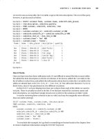
although it can be done. This example uses the item and stock tables in our sample database.
As you will remember, all the items that we might sell are held in the item table, and only items
we actually stock are held in the stock table, as illustrated in Figure 7-2.
Figure 7-2. Schema for the item and stock tables
Let’s work through a solution, beginning with using only the SQL we know so far. Let’s try
a simple SELECT, joining the two tables:
bpsimple=# SELECT i.item_id, s.quantity FROM item i, stock s
bpsimple-# WHERE i.item_id = s.item_id;
item_id | quantity
+
1 | 12
2 | 2
4 | 8
5 | 3
7 | 8
8 | 18
10 | 1
(7 rows)

bpsimple=#
It’s easy to see (since we happen to know that our item_ids in the item table are sequential,
with no gaps), that some item_ids are missing. The rows that are missing are those relating to
items that we do not stock, since the join between the item and stock tables fails for these rows,
as the stock table has no entry for that item_id. We can find the missing rows, using a subquery
and an IN clause:
MatthewStones_4789C07.fm Page 196 Tuesday, February 1, 2005 7:33 AM
CHAPTER 7 ■ ADVANCED DATA SELECTION
197
bpsimple=# SELECT i.item_id FROM item i
bpsimple-# WHERE i.item_id NOT IN
bpsimple-# (SELECT i.item_id FROM item i, stock s
bpsimple(# WHERE i.item_id = s.item_id);
item_id

3
6
9
11
(4 rows)
bpsimple=#
We might translate this as, “Tell me all the item_ids in the item table, excluding those that
also appear in the stock table.”
The inner SELECT statement is simply the one we used earlier, but this time, we use the list
of item_ids it returns as part of another SELECT statement. The main SELECT statement lists all
the known item_ids, except that the WHERE NOT IN clause removes those item_ids found in the
subquery.
So now we have a list of item_ids for which we have no stock, and a list of item_ids for
which we do have stock, but retrieved using different queries. What we need to do now is glue
the two lists together, which is the job of the UNION join. However, there is a slight problem. Our

first statement returns two columns, item_id and quantity, but our second SELECT returns only
item_ids, as there is no stock for these items. We need to add a dummy column to the second
SELECT, so it has the same number and types of columns as the first SELECT. We will use NULL.
Here is our complete query:
SELECT i.item_id, s.quantity FROM item i, stock s WHERE i.item_id = s.item_id
UNION
SELECT i.item_id, NULL FROM item i WHERE i.item_id NOT IN
(SELECT i.item_id FROM item i, stock s WHERE i.item_id = s.item_id);
This looks a bit complicated, but let’s give it a try:
bpsimple=# SELECT i.item_id, s.quantity FROM item i, stock s
bpsimple-# WHERE i.item_id = s.item_id
bpsimple-# UNION
bpsimple-# SELECT i.item_id, NULL FROM item i
bpsimple-# WHERE i.item_id NOT IN
bpsimple-# (SELECT i.item_id FROM item i, stock s WHERE i.item_id = s.item_id);
item_id | quantity
+
1 | 12
2 | 2
3 |
4 | 8
5 | 3
6 |
MatthewStones_4789C07.fm Page 197 Tuesday, February 1, 2005 7:33 AM
198
CHAPTER 7
■ ADVANCED DATA SELECTION
7 | 8
8 | 18
9 |

10 | 1
11 |
(11 rows)
bpsimple=#
In the early days of SQL, this was pretty much the only way of solving this type of problem,
except that SQL89 did not allow the NULL we used in the second SELECT statement as a column.
Fortunately, most vendors allowed the NULL, or life would have been even more difficult. If we
had not been allowed to use NULL, we would have used 0 (zero) as the next best alternative. NULL
is better because 0 is potentially misleading; NULL will always be blank.
To get around this rather complex solution for what is a fairly common problem, vendors
invented outer joins. Unfortunately, because this type of join did not appear in the standard, all
the vendors invented their own solutions, with similar ideas but different syntax.
Oracle and DB2 used a syntax with a + sign in the WHERE clause to indicate that all values of
a table must appear (the preserved table), even if the join failed. Sybase used *= in the WHERE
clause to indicate the preserved table. Both of these syntaxes are reasonably straightforward,
but unfortunately different, which is not good for the portability of your SQL.
When the SQL92 standard appeared, it specified a very general-purpose way of implementing
joins, resulting in a much more logical system for outer joins. Vendors have, however, been
slow to implement the new standard. (Sybase 11 and Oracle 8, which both came out after the
SQL92 standard, did not support it, for example.) PostgreSQL implemented the SQL92 standard
method starting in version 7.1.
■Note If you are running a version of PostgreSQL prior to version 7.1, you will need to upgrade to try the
last examples in this chapter. It’s probably worth upgrading if you are running a version older than 7.x anyway,
as version 8 has significant improvements over older versions.
The SQL92 syntax for outer joins replaces the WHERE clause we are familiar with, using an ON
clause for joining tables, and adds the LEFT OUTER JOIN keywords. The syntax looks like this:
SELECT columns FROM table1
LEFT OUTER JOIN table2 ON table1.column = table2.column
The table name to the left of LEFT OUTER JOIN is always the preserved table, the one from
which all rows are shown.

So, now we can rewrite our query, using this new syntax:
SELECT i.item_id, s.quantity FROM item i
LEFT OUTER JOIN stock s ON i.item_id = s.item_id;
Does this look almost too simple to be true? Let’s give it a go:
MatthewStones_4789C07.fm Page 198 Tuesday, February 1, 2005 7:33 AM
CHAPTER 7 ■ ADVANCED DATA SELECTION
199
bpsimple=# SELECT i.item_id, s.quantity FROM item i
bpsimple-# LEFT OUTER JOIN stock s ON i.item_id = s.item_id;
item_id | quantity
+
1 | 12
2 | 2
3 |
4 | 8
5 | 3
6 |
7 | 8
8 | 18
9 |
10 | 1
11 |
(11 rows)
bpsimple=#
As you can see, the answer is identical to the one we got from our original version.
You can see why most vendors felt they needed to implement an outer join, even though it
wasn’t in the original SQL89 standard.
There is also the equivalent RIGHT OUTER JOIN, but the LEFT OUTER JOIN is used more often
(at least for Westerners, it makes more sense to list the known items down the left side of the
output rather than the right).

Try It Out: Use a More Complex Condition
The simple LEFT OUTER JOIN we have used is great as far as it goes, but how do we add more
complex conditions?
Suppose we want only rows from the stock table where we have more than two items in stock,
and overall, we are interested only in rows where the cost price is greater than 5.0. This is quite
a complex problem, because we want to apply one rule to the item table (that cost_price > 5.0)
and a different rule to the stock table (quantity > 2), but we still want to list all rows from the
item table where the condition on the item table is true, even if there is no stock at all.
What we do is combine ON conditions that work on left-outer-joined tables only, with WHERE
conditions that limit all the rows returned after the table join has been performed.
The condition on the stock table is part of the outer join. We don’t want to restrict rows
where there is no quantity, so we write this as part of the ON condition:
ON i.item_id = s.item_id AND s.quantity > 2
For the item condition, which applies to all rows, we use a WHERE clause:
WHERE i.cost_price > cast(5.0 AS numeric(7,2));
Putting them both together, we get this:
bpsimple=# SELECT i.item_id, i.cost_price, s.quantity FROM item i
bpsimple-# LEFT OUTER JOIN stock s
MatthewStones_4789C07.fm Page 199 Tuesday, February 1, 2005 7:33 AM