APPLICATIONS OF MATLAB IN SCIENCE AND ENGINEERING - PART 5 docx
Bạn đang xem bản rút gọn của tài liệu. Xem và tải ngay bản đầy đủ của tài liệu tại đây (935.53 KB, 53 trang )
Low-Noise, Low-Sensitivity Active-RC Allpole Filters Using MATLAB Optimization
201
(Moschytz & Horn, 1981). In Figure 2(b) there is a simplified version of the same circuit with
the voltage-controlled voltage source (VCVS) having voltage gain
. For an ideal opamp in
the non-inverting mode it is given by
1/
FG
RR
. (10)
Note that the voltage gain
of the class-4 circuit is positive and larger than or equal to unity.
Voltage transfer function for the filters in Figure 2 expressed in terms of the coefficients a
i
(i=0, 1, 2) is given by
0
2
10
()
()
()
out
g
Va
Ns
Ts K
VDs
sasa
, (11a)
and in terms of the pole frequency
p
, the pole Q, q
p
and the gain factor K by:
2
22
()
p
out
p
g
p
p
V
Ts K
V
ss
q
, (11b)
where
2
0
1212
11 2 22 11
1
1212
1212
11 2 22 11
1
,
()
,
,
()
.
p
p
p
p
a
RRCC
RC C RC RC
a
q RRCC
RRCC
q
RC C RC RC
K
(11c)
(a) (b)
Fig. 2. Second-order Sallen and Key LP active-RC filter. (a) With ideal opamp having
feedback resistors R
F
and R
G
, and nodes for transfer-function calculus. (b) Simplified circuit
with the gain element replaced by VCVS
.
To calculate the voltage transfer function T(s)=V
out
(s)/V
g
(s) of the Biquad in Figure 2(a),
consider the following system of nodal equations (note that the last equation represents the
opamp):
Applications of MATLAB in Science and Engineering
202
1
12 1351
112 2
23 2
22
35
35 5
(1)
111 1
(2) 0
11
(3) 0
11 1
(4) 0
(5) ( ) , , 0, 0.
g
FG F
out
VV
VV sCVVsC
RRR R
VV sC
RR
VV
RR R
AV V V V A i i
(12)
The system of Equations (12) can be solved using 'Symbolic toolbox' in Matlab. The
following Matlab code solves the system of equations:
i.
Matlab command syms defines symbolic variables in Matlab's workspace:
syms A R1 R2 C1 C2 RF RG s Vg V1 V2 V3 V4 V5;
ii. Matlab command solve is used to solve analytically above system of five Equations
(12) for the five voltages V
1
to V
5
as unknowns. The unknowns are defined in the last
row of command
solve. Note that all variables used in solve are defined as symbolic.
CircuitEquations=solve(
'V1=Vg',
'-V1*1/R1 + V2*(1/R1+1/R2+s*C1)-V3*1/R2 - V5*s*C1=0',
'-V2*1/R2 + V3*(1/R2+s*C2)=0',
'V4*(1/RG+1/RF)-V5/RF=0',
'(V3-V4)*A =V5',
'V1','V2','V3','V4','V5');
iii. Once all variables are known simple symbolic division of V
5
/V
1
yields the desired
transfer function (limit value for A∞ has to be applied, as well):
Tofs=CircuitEquations.V5/CircuitEquations.V1;
Tofsa=limit(Tofs,A,Inf);
Another way of presentation polynomials is by collecting all coefficients that multiply
's':
Tofsc=collect(Tofsa,s);
iv. Transfer function coefficients and parameters readily follow.
To obtain coefficients, it is useful to separate numerator and denominator using the
following command:
[numTa,denTa]=numden(Tofsa);
syms a2 a1 a0 wp qp k;
denLP2=coeffs(denTa,s)/RG;
numLP2=coeffs(numTa,s)/RG;
Now coefficients follow
Low-Noise, Low-Sensitivity Active-RC Allpole Filters Using MATLAB Optimization
203
a0=denLP2(1)/denLP2(3);
a1=denLP2(2)/denLP2(3);
a2=denLP2(3)/denLP2(3);
And parameters
k=numLP2;
wp=sqrt(a0);
qp=wp/a1;
Typing command whos we obtain the following answer about variables in Matlab
workspace:
>> whos
Name Size Bytes Class
A 1x1 126 sym object
C1 1x1 128 sym object
C2 1x1 128 sym object
CircuitEquations 1x1 2828 struct array
Tofs 1x1 496 sym object
Tofsa 1x1 252 sym object
Tofsc 1x1 248 sym object
R1 1x1 128 sym object
R2 1x1 128 sym object
RF 1x1 128 sym object
RG 1x1 128 sym object
V1 1x1 128 sym object
V2 1x1 128 sym object
V3 1x1 128 sym object
V4 1x1 128 sym object
V5 1x1 128 sym object
Vg 1x1 128 sym object
a0 1x1 150 sym object
a1 1x1 210 sym object
a2 1x1 126 sym object
denTa 1x1 232 sym object
denLP2 1x3 330 sym object
k 1x1 144 sym object
numTa 1x1 134 sym object
numLP2 1x1 144 sym object
qp 1x1 254 sym object
s 1x1 126 sym object
wp 1x1 166 sym object
Grand total is 1436 elements using 7502 bytes
It can be seen that all variables that are defined and calculated so far are of symbolic type.
We can now check the values of the variables. For example we are interested in voltage
transfer function
Tofsa. Matlab gives the following answer, when we invoke the variable:
>> Tofsa
Tofsa =
(RF+RG)/(s*C2*R2*RG+R2*s^2*C1*R1*C2*RG-s*C1*R1*RF+RG+R1*s*C2*RG)
Applications of MATLAB in Science and Engineering
204
The command pretty presents the results in a more beautiful way.
>> pretty(Tofsa)
RF + RG
2
s C2 R2 RG + R2 s C1 R1 C2 RG - s C1 R1 RF + RG + R1 s C2 RG
Or we could invoke variable Tofsc (see above that Tofsc is the same as Tofsa, but with
collected coefficients that multiply powers of 's').
>> pretty(Tofsc)
RF + RG
2
R2 s C1 R1 C2 RG + (C2 R2 RG - C1 R1 RF + R1 C2 RG) s + RG
Other variables follow using pretty command.
>> pretty(a0)
1
R2 C1 R1 C2
>> pretty(a1)
C2 R2 RG - C1 R1 RF + R1 C2 RG
RG R2 C1 R1 C2
>> pretty(a2)
1
>> pretty(wp)
/ 1 \1/2
| |
\R2 C1 R1 C2/
>> pretty(qp)
/ 1 \1/2
| | RG R2 C1 R1 C2
\R2 C1 R1 C2/
C2 R2 RG - C1 R1 RF + R1 C2 RG
>> pretty(k)
RF + RG
RG
Next, according to simplified circuit in Figure 2(b) having the replacement of the gain
element by
defined in (10), we can substitute values for R
F
and R
G
using the command
Low-Noise, Low-Sensitivity Active-RC Allpole Filters Using MATLAB Optimization
205
subs
and obtain simpler results [in the following example we perform substitution R
F
R
G
(
–1)]. New symbolic variable is beta
>> syms beta
>> a1=subs(a1,RF,'(beta-1)*RG');
>> pretty(a1)
C2 R2 RG - C1 R1 (beta - 1) RG + R1 C2 RG
RG R2 C1 R1 C2
Note that we have obtained R
G
both in the numerator and denominator, and it can be
abbreviated. To simplify equations it is possible to use several Matlab commands for
simplifications. For example, to rewrite the coefficient a
1
in several other forms, we can use
commands for simplification, such as:
>> pretty(simple(a1))
1 beta 1 1
- + +
C1 R1 R2 C2 R2 C2 R2 C1
>> pretty(simplify(a1))
-C2 R2 + C1 R1 beta - C1 R1 - R1 C2
-
R2 C1 R1 C2
The final form of the coefficient a
1
is the simplest one, and is the same as in (11c) above.
Using the same Matlab procedures as presented above, we have calculated all coefficients
and parameters of the different filters' transfer functions in this Chapter.
If we want to calculate the numerical values of coefficients a
i
(i=0, 1, 2) when component
values are given, we simply use
subs command. First we define the (e.g. normalized)
numerical values of components in the Matlab’s workspace, and then we invoke
subs:
>> R1=1;R2=1;C1=0.5;C2=2;
>> a0val=subs(a0)
a0val =
1
>> whos a0 a0val
Name Size Bytes Class
a0 1x1 150 sym object
a0val 1x1 8 double array
Grand total is 15 elements using 158 bytes
Note that the new variable a0val is of the double type and has numerical value equal to 1,
whereas the
symbolic variable a0 did not change its type. Numerical variables are of type
double.
Applications of MATLAB in Science and Engineering
206
3.2 Drawing amplitude- and phase-frequency characteristics of transfer function
using symbolic and numeric calculations in Matlab
Suppose we now want to plot Bode diagram of the transfer function, e.g. of the Tofsa, using
the symbolic solutions already available (see above). We present the usage of the Matlab in
numeric way, as well. Suppose we already have symbolic values in the Workspace such as:
>> pretty(Tofsa)
RF + RG
2
RG - C1 R1 RF s + C2 R1 RG s + C2 R2 RG s + C1 C2 R1 R2 RG s
Define set of element values (normalized):
>> R1=1;R2=1;C1=1;C2=1;RG=1;RF=1.8;
Now the variables representing elements R
1
, R
2
, C
1
, C
2
, R
G
, and R
F
changed in the workspace
to
double and have values; they become numeric. Substitute those elements into transfer
function
Tofsa using the command subs.
>> Tofsa1=subs(Tofsa);
>> pretty(Tofsa1)
14
/ 2 s \
5 | s + - + 1 |
\ 5 /
Note that in new transfer function Tofsa1 an independent variable is symbolic variable s.
To calculate the amplitude-frequency characteristic, i.e., the magnitude of the filter's voltage
transfer function we first have to define frequency range of
, as a vector of discrete values
in
wd, make substitution s=j
into T(s) (in Matlab represented by Tofsa1) to obtain T(j
),
and finally calculate absolute value of the magnitude in dB by
(
)=20 log T(j
). The
phase-frequency characteristic is
(
)=arg T(j
) and is calculated using atan2(). This can
be performed in following sequence of commands:
wd = logspace(-1,1,200);
ad1 = subs(Tofsa1,s,i*wd);
Alphad=20*log10(abs(ad1));
semilogx(wd, Alphad, 'g-');
axis([wd(1) wd(end) -40 30]);
title('Amplitude Characteristic');
legend('Circuit 1 (normalized)');
xlabel('Frequency /rad/s');ylabel('Magnitude / dB');
grid;
Phid=180/pi*atan2(imag(ad1),real(ad1));
semilogx(wd, Phid, 'g-');
axis([wd(1) wd(end) -180 0]);
title('Phase Characteristic');
legend('Circuit 1 (normalized)');
xlabel('Frequency /rad/s');ylabel('Phase / deg');
grid;
Low-Noise, Low-Sensitivity Active-RC Allpole Filters Using MATLAB Optimization
207
Commands are self-explanatory. The amplitude- and phase-frequency characteristics thus
obtained are shown in Figure 3. Note that we have generated vectors of values
wd, Alphad
and
Phid to be plotted in logarithmic scale by the command semilogx (instead, we could
have used command
plot to generate linear axis).
The next example defines new set of second-order LP filter element values (those are
obtained when above normalized elements are denormalized to the frequency
0
=2
8610
3
rad/s and impedance R
0
=37k; see in (Jurisic et al., 2008) how):
>> R1=37e3;R2=37e3;C1=50e-12;C2=50e-12;RG=1e4;RF=1.8e4;
Those element values were calculated starting from transfer function parameters
p
=
2
8610
3
rad/s and q
p
=5 and are represented as example 1) non-tapered filter (
=1, and r=1)
(see Equation (18) and Table 3 in Section 4 below). We refer to those values as 'Circuit 1'.
>> Tofsa2=subs(Tofsa);
>> pretty(Tofsa2)
28000
2
800318296602402496323046008438980478515625 s 4473025532574128109375 s
+ + 10000
23384026197294446691258957323460528314494920687616 1208925819614629174706176
(a) (b)
Fig. 3. Transfer-function (a) magnitude and (b) phase for Circuit 1 (normalized).
It is seen that the denormalized-transfer-function presentation in symbolic way is not very
useful. It is possible rather to use numeric and vector presentation of the
Tofsa2. First we
have to separate numerator and denominator of
Tofsa2 by typing:
>> [num2, den2]=numden(Tofsa2);
then we have to convert obtained symbolic data of num2 and den2 into vectors n2 and
d2:
Applications of MATLAB in Science and Engineering
208
>> n2=sym2poly(num2)
n2 =
6.5475e+053
>> d2=sym2poly(den2)
d2 =
1.0e+053 *
0.0000 0.0000 2.3384
and finally use command tf to write transfer function which uses vectors with numeric
values:
>> tf(n2,d2)
Transfer function:
6.548e053
8.003e041 s^2 + 8.652e046 s + 2.338e053
If we divide numerator and denominator by the coefficient of s
2
in the denominator, i.e.,
d2(1), we have a more appropriate form:
>> tf(n2/d2(1),d2/d2(1))
Transfer function:
8.181e011
s^2 + 1.081e005 s + 2.922e011
Obviously, the use of Matlab (numeric) vectors provides a more compact and useful
representation of the denormalized transfer function.
Finally, note that when several (N) filter sections are connected in a cascade, the overall
transfer function of that cascade can be very simply calculated by symbolic multiplication of
sections' transfer functions
T
i
(s) (i=1, , N), i.e. T=T1**TN, if T
i
(s) are defined in a
symbolic way. On the other hand, if numerator and denominator polynomials of
T
i
(s) are
defined numerically (i.e. in a vector form), a more complicated procedure of multiplying
vectors using (convolution) command
conv should be used.
3.3 Calculating noise transfer function using symbolic calculations in Matlab
Using the noise models for the resistors and opamps from Figure 1, we obtain noise spot
sources shown in Figure 4(a).
(a) (b)
Fig. 4. (a) Noise sources for second-order LP filter. (b) Noise transfer function for
contribution of R
1
.
Low-Noise, Low-Sensitivity Active-RC Allpole Filters Using MATLAB Optimization
209
The noise transfer functions as in (3) T
x
(s)=V
out
/N
x
from each equivalent voltage or current
noise source to the output of the filter in Figure 4(a) has to be evaluated.
As a first example we find the contribution of noise produced by resistor R
1
at the filter's
output. We have to calculate the transfer resistance T
i,R1
(s)=V
out
(s)/I
nR1
(s). According to
Figure 4(b) we write the following system of nodal equations:
1
12 13511
112 2
23 2
22
45
34 5
(1) 0
111 1
(2)
11
(3) 0
11 1
(4) 0
(5)
nR
FG F
V
V V sC V V sC I
RRR R
VV sC
RR
VV
RR R
AV V V
(13)
The system of Equations (13) can be solved using Matlab Symbolic toolbox in the same way
as the system of Equations (12) presented above. The following Matlab code solves the
system of Equations (13):
CircuitEquations=solve(
'V1=0',
'-V1*1/R1 + V2*(1/R1+1/R2+s*C1)-V3*1/R2 - V5*s*C1=InR1',
'-V2*1/R2 + V3*(1/R2+s*C2)=0',
'V4*(1/RG+1/RF)-V5/RF=0',
'(V3-V4)*A =V5',
'V1','V2','V3','V4','V5');
IR1ofs=CircuitEquations.V5/InR1;
IR1ofsa=limit(IR1ofs,A,Inf);
[numIR1a,denIR1a]=numden(IR1ofsa);
syms a2 a1 a0 b0
denIR1=coeffs(denIR1a,s)/RG;
numIR1=coeffs(numIR1a,s)/RG;
%Coefficients of the transfer function
a0=denIR1(1)/denIR1(3);
a1=denIR1(2)/denIR1(3);
a2=denIR1(3)/denIR1(3);
b0=numIR1/denIR1(3);
In Matlab workspace we can check the value of each coefficient calculated by above
program, simply, by typing the corresponding variable. For example, we present the value
of the coefficient b
0
in the numerator by typing:
>> pretty(b0)
RF + RG
| |
C1 C2 R2 RG
The coefficients a
0
, a
1
and a
2
are the same as those of the voltage transfer function calculated in
Section 3.1 above, which means that two transfer functions have the same denominator, i.e.,
D(s). Thus, the only useful data is the coefficient b
0
. The transfer resistance T
i,R1
(s) is obtained.
Applications of MATLAB in Science and Engineering
210
The noise transfer functions of all noise spot sources in Figure 4(a) have been calculated
and presented in Table 1 in the same way as T
i,R1
(s) above. We use current sources in the
resistor noise model. N
x
is either the voltage or current noise source of the element denoted
by x.
3.4 Drawing output noise spectral density of active-RC filters using numeric
calculations in Matlab
Noise transfer functions for second-order LP filter, generated using Matlab in Section 3.3, are
shown in Table 1. We can retype them and use Matlab in only numerical mode to calculate
noise spectral density curves at the output, that are defined as a square root of (3). Define set of
element values (Circuit 1)
>> R1=37e3;R2=37e3;C1=50e-12;C2=50e-12;RG=1e4;RF=1.8e4;
N
x
T
x
(s)
V
g
1212
1
()Ds
RRCC
i
nR1
, i
nR11
, i
nR12
212
1
()Ds
RCC
i
nR2
2112
11
()sDs
CRCC
i
na1
2112212
11 1
()sDs
C RCC RCC
i
na2
, i
nRG
, i
nRF
, e
na
*
2
22 12 11
1212 1212
1
()
F
RC RC RC
Rs s Ds
RRCC RRCC
2
22 12 11
1212 1212
(1 ) 1
()
RC RC RC
Ds s s
RRCC RRCC
Table 1. Noise transfer functions for second-order LP filter (*e
na
has
instead –R
F
).
We draw the curve:
% FREQUENCY RANGE
Nfreq=200;
Fstart=1e4; %Hz
Fstop=1e6; %Hz
fd =logspace(log10(Fstart),log10(Fstop),Nfreq);
% NOISE SOURCES at temperature T=295K (22 deg C)
IR1=sqrt(4*1.38e-23*295/R1);
IR2=sqrt(4*1.38e-23*295/R2);
IRF=sqrt(4*1.38e-23*295/RF);
IRG=sqrt(4*1.38e-23*295/RG);
EP=17e-9;
IP=0.01e-12;
IM=0.01E-12;
Low-Noise, Low-Sensitivity Active-RC Allpole Filters Using MATLAB Optimization
211
% TRANSFER FUNCTIONS OF EVERY NOISE SOURCE
D=1/(R1*R2*C1*C2) - (fd*2*pi).^2 +
i*(fd*2*pi)*(1/(R1*C1)+1/(R2*C1)-RF/(R2*C2*RG));
H=(1/(R1*R2*C1*C2)*(1+RF/RG))./D;
numerator=(1/(R1*R2*C1*C2)*(1+RF/RG))*conj(D);
phase=atan(imag(numerator)./real(numerator));
TR1=(1/(R2*C1*C2)*(1+RF/RG))./D;
TR2=((1+RF/RG)*(1/(R1*C1*C2)+i*(fd*2*pi)*1/C2))./D;
TIP=((1+RF/RG)*(1/(R1*C1*C2)+1/(R2*C1*C2)+i*(fd*2*pi)*1/C2))./D;
TIM=-RF*(1/(R1*R2*C1*C2)-(fd*2*pi).^2 +
i*(fd*2*pi)*(1/(R1*C1)+1/(R2*C1)+1/(R2*C2)))./D;
TRG=TIM;
TRF=TIM;
TEP=(1+RF/RG)*(1/(R1*R2*C1*C2)
(fd*2*pi).^2+i*(fd*2*pi)*(1/(R1*C1)+1/(R2*C1)+1/(R2*C2)))./D;
% SQUARES OF TRANS. FUNCTIONS
TR1A =(abs(TR1)).^2;
TR2A =(abs(TR2)).^2;
TIPA =(abs(TIP)).^2;
TIMA =(abs(TIM)).^2;
TRGA =TIMA;
TRFA =TIMA;
TEPA =(abs(TEP)).^2;
% SPECTRAL DENSITY OF EVERY NOISE SOURCE
UR1 =TR1A*IR1^2;
UR2 =TR2A*IR2^2;
UIP =TIPA*IP^2;
UIM =TIMA*IM^2;
UEP =TEPA*EP^2;
URG =TRGA*IRG^2;
URF =TRFA*IRF^2;
% OVERALL SPECTRAL DENSITY PLOT
U2=sqrt(UR1+UR2+UIP+UIM+URF+UEP+URG);
semilogx(fd,U2,'k-');
titletext=sprintf('Output Noise');title(titletext);
xlabel('Frequency / kHz');
ylabel('Noise Spectral Density / \muV/\surdHz');
axis ([fd(1) fd(Nfreq) 0 3e-6]); grid;
% Numerical integration of Total Noise Power at the Output (RMS)
Eno = sqrt(sum(U22(1:Nfreq))/(Nfreq-1)*(fd(Nfreq)-fd(1)));
To draw the second curve, apply the following method. Define the second set of element
values, that are represented as example 4) ideally tapered filter (
=4, and r=4), (see Equation
(18) and Table 3 in Section 4 below). We refer to those values as 'Circuit 2'.
>> R1=23.1e3;R2=92.4e3;C1=80e-12;C2=20e-12;RG=1e4;RF=1.05e4;
>> hold on;
>> redo all above equations; use 'r ' for the second curve shape
>> hold off;
>> legend('Circuit 1', 'Circuit 2');
Output noise spectral density is shown in Figure 5.
Furthermore, two values of rms voltages E
no
(representing total noise power at the output or
the noise floor) as defined by the square root of (4), have been calculated as a result of
Applications of MATLAB in Science and Engineering
212
numerical integration in Matlab code given above, and they are as follows: E
no1
=176.0 V
(Circuit 1 or example #1 in Table 3) and E
no2
=127.7 V (Circuit 2 or example #4 in Table 3).
They are shown in the last column of Table 3, in Section 4.
For all filter examples the rms total output noise E
no
was calculated numerically using
Matlab and presented in the last column of Tables.
To plot output noise spectral density and calculate total output noise voltage it was easy
to retype the noise transfer function expressions from Table 1 in Matlab code. In the
following Section 3.5 it is shown that retyping of long expressions is sometimes
unacceptable (e.g. to calculate the sensitivity). Then we have another option to use Matlab in
symbolic mode.
Fig. 5. Output noise spectral density of Circuit 1 and Circuit 2 (denormalized).
3.5 Sensitivity characteristic of active-RC filter using both symbolic and numeric
calculations in Matlab
To efficiently calculate multi-parametric sensitivity in (9), we use a mixture of symbolic and
numeric capabilities of Matlab.
Suppose F in (7)–(9) is our transfer function T(s)=N(s)/D(s) defined by (11), where x
k
are
elements R
1
, R
2
, C
1
, C
2
, R
F
and R
G
. We will use previous symbolic results of transfer functions
numerator
numLP2 and denominator denLP2, and Matlab operation of symbolic
differentiation
diff to produce relative sensitivity in (8). To calculate the transfer function
sensitivity as defined by (8) we will also apply the following rule:
() () ()
kk k
T
j
N
j
D
j
xxx
SSS
. (14)
To construct (14), we proceed as follows. The following code reveal numerator and
denominator as function of components. (Division of both numerator and denominator by
R
G
is just to have nicer presentation.) First we make the substitution s=j
into N(s) and D(s).
Then we have to produce absolute values of N(j
) and D(j
). In the subsequent step we
perform symbolic differentiation using Matlab command
diff or the operator D.
Low-Noise, Low-Sensitivity Active-RC Allpole Filters Using MATLAB Optimization
213
>> den=simplify(denTa/RG);
>> pretty(den)
2 C1 R1 RF s
C2 R1 s + C2 R2 s + C1 C2 R1 R2 s - + 1
RG
>> denofw = subs(den,s,i*wd)
denofw =
C2*R2*wd*i - C1*C2*R1*R2*wd^2 + 1 - (C1*R1*RF*wd*i)/RG + C2*R1*wd*i
(To calculate all components and frequency values as real variables we have to retype real
and imaginary parts of
denofw.)
>> syms wd;
>> redenofw= - C1*C2*R1*R2*wd^2 + 1;
>> imdenofw= C2*R2*wd - (C1*R1*RF*wd)/RG + C2*R1*wd;
>> absden=sqrt(redenofw^2+imdenofw^2);
>> pretty(absden)
/ / C1 R1 RF wd \2 2 2 \1/2
| | C2 R1 wd + C2 R2 wd - | + (C1 C2 R1 R2 wd - 1) |
\ \ RG / /
>> SDR1=diff(absden,R1)*R1/absden;
>> pretty(SDR1)
/ / C1 RF wd \ / C1 R1 RF wd \ 2 2 \
R1 | 2 | C2 wd - | | C2 R1 wd + C2 R2 wd - | + 2 C1 C2 R2 wd (C1 C2 R1 R2 wd - 1) |
\ \ RG / \ RG / /
/ / C1 R1 RF wd \2 2 2 \
2 | | C2 R1 wd + C2 R2 wd - | + (C1 C2 R1 R2 wd - 1) |
\ \ RG / /
The same calculus (with simpler results) can be done for the numerator:
>> num=simplify(numTa/RG);
>> pretty(num)
RF
+ 1
RG
>> numofw = subs(num,s,i*wd)
numofw =
RF/RG + 1
>> renumofw= RF/RG + 1;
>> imnumofw= 0;
>> absnum=sqrt(renumofw^2+imnumofw^2);
Applications of MATLAB in Science and Engineering
214
>> pretty(absnum)
/ / RF \2 \1/2
| | + 1 | |
\ \ RG / /
>> SNR1=diff(absnum,R1)*R1/absnum;
>> pretty(SNR1)
0
Sensitivity of the numerator to R
1
is zero. We have obviously obtained too long result to be
analyzed by observation. We continue to form sensitivities to all remaining components in
symbolic form.
>> SDR2=diff(absden,R2)*R2/absden;
>> SDC1=diff(absden,C1)*C1/absden;
>> SDC2=diff(absden,C2)*C2/absden;
>> SDRF=diff(absden,RF)*RF/absden;
>> SDRG=diff(absden,RG)*RG/absden;
>> SNR2=diff(absnum,R2)*R2/absnum;
>> SNC1=diff(absnum,C1)*C1/absnum;
>> SNC2=diff(absnum,C2)*C2/absnum;
>> SNRF=diff(absnum,RF)*RF/absnum;
>> SNRG=diff(absnum,RG)*RG/absnum;
By application of rule (14), we form sensitivities to each component, whose squares we
finally have to sum, and form (9).
>>SCH=(SNR1-SDR1)^2+(SNR2-SDR2)^2+(SNC1-SDC1)^2+(SNC2-SDC2)^2+
(SNRF-SDRF)^2+(SNRG-SDRG)^2;
The resulting analytical form of multi-parametric sensitivity is as follows:
>> SigmaAlpha=sqrt(SCH)*0.01*8.68588964;
The multiplication by 0.01 defines the standard deviation of all passive elements
x
in (9) to
be 1%. The multiplication by 8.68588965 converts the standard deviation
F
in (9) into
decibels.
When typing
SigmaAlpha in Matlab's workspace, a very large symbolic expression is
obtained. We do not present it here (it is not recommended to try!). Because it is too large
neither is it useful for an analytical investigation, nor can it be retyped, nor presented in
table form. Instead we will substitute in this large analytical expression for
SigmaAlpha
component values and draw it numerically. This has more sense.
Define first set of element values (Circuit 1 with equal capacitors and equal resistors):
>> R1=37e3;R2=37e3;C1=50e-12;C2=50e-12;RG=1e4;RF=1.8e4;
Low-Noise, Low-Sensitivity Active-RC Allpole Filters Using MATLAB Optimization
215
By equating to values, elements changed in the workspace to double and they have become
numeric. Substitute those elements into
SigmaAlpha.
>> Schoefler1=subs(SigmaAlpha);
Note that in new variable Schoefler1 independent variable is symbolic wd. To calculate
its magnitude, we have to define first the frequency range of
, as a vector of discrete values
in
wd. When the frequency in Hz is defined, we have to multiply it by 2
. The frequency
assumed ranges from 10kHz to 1MHz.
>> fd = logspace(4,6,200);
>> wd = 2*pi*fd;
>> Sch1 = subs(Schoefler1,wd);
>> semilogx(fd, Sch1, 'g ');
>> title('Multi-Parametric Sensitivity');
>> xlabel('Frequency / kHz');
ylabel('\sigma_{\alpha} / dB');
>> legend('Circuit 1');
>> axis([fd(1) fd(end) 0 2.5])
>> grid;
This is all needed to plot the sensitivity curve of Circuit 1.
To add the second example, we set the element values of Circuit 2 in the Matlab workspace:
>> R1=23.1e3;R2=92.4e3;C1=80e-12;C2=20e-12;RG=1e4;RF=1.05e4;
Then we substitute symbolic elements (components) in the SigmaAlpha with the numeric
values of components in the workspace to obtain new numeric vales for sensitivity
>> Schoefler2=subs(SigmaAlpha);
>> Sch2 = subs(Schoefler2,wd);
Finally, to draw both curves we type
>> semilogx(fd, Sch1, 'k-', fd, Sch2, 'r ');
>> title('Multi-Parametric Sensitivity');
>> xlabel('Frequency / kHz');
ylabel('\sigma_{\alpha} / dB');
>> legend('Circuit 1', 'Circuit 2');
>> axis([fd(1) fd(end) 0 2.5])
>> grid;
Sensitivity curves of Circuit 1 and Circuit 2 are shown in Figure 6. Recall that both circuits
realize the same transfer-function magnitude which is shown in Figure 3(a) above. Note that
only several lines of Matlab instructions have to be repeated, and none of large analytical
expressions have to be retyped.
In the following Chapter 4, we will use Matlab routines presented so far to construct
examples of different filter designs. According to the results obtained from noise and
sensitivity analyses we prove the optimum design.
Applications of MATLAB in Science and Engineering
216
Fig. 6. Standard deviation of magnitudes of Circuit 1 and Circuit 2 (sensitivity).
4. Application to second- and third-order LP, BP, and HP filters
4.1 Second-order Biquads
Consider the second-order Biquads that realize LP, HP and BP transfer functions, shown in
Figure 7. Those are the Biquads that are recommended as high-quality building blocks; see
(Moschytz & Horn, 1981; Jurisic et al., 2010b, 2010c). In (Moschytz & Horn, 1981) only the
design procedure for min. GSP is given (and by that providing the minimum active
sensitivity design). On the basis of component ratios in the passive, frequency-dependent
feedback network of the Biquads in Figure 7, defined by:
12 21
/, /CCrRR
, (15)
the detailed step-by-step design of those filters, in the form of cookbook, for optimum
passive and active sensitivities as well as low noise is considered in (Jurisic et al., 2010b,
2010c). The optimum design is presented in Table 1 in (Jurisic et al., 2010c) and is
programmed using Matlab.
Note that the Biquads in Figure 7 shown vertically are related by the complementary
transformation, whereas those shown horizontally are RC–CR duals of each other. Thus,
complementary circuits are LP (class-4: positive feedback) and BP-C (class-3: negative
feedback), as well as HP (class-4) and BP-R (class-3). In class-4 case there is
, whereas in
class-3 there is
, that are related by:
1/ 1/ 1
. (16)
Dual Biquads in Figure 7 are LP and HP (class-4), as well as BP-C and BP-R (class-3); they
belong to the same class.
Low-Noise, Low-Sensitivity Active-RC Allpole Filters Using MATLAB Optimization
217
RC–CR Duality
Positive feedback
Complementary Transformation
(a) Low pass (b) High pass
Negative feedback
(c) Band pass -Type C (d) Band pass -Type R
Fig. 7. Second-order LP, HP and BP active-RC filters with impedance scaling factors r and
.
Voltage transfer functions for all the filters shown in Figure 7 in terms of the pole frequency
p
, the pole Q, q
p
and the gain factor K, are defined by:
2
22
1
() ()
()
()
p
p
p
VNs ns
Ts K
VDs
ss
q
, (17a)
where numerators n(s) are given by:
22
() , () , ()
HP BP
p
LP
p
nss ns sns
. (17b)
Parameters
p
, q
p
and K, as functions of filter components, are given in Table 2. They are
calculated using Matlab procedures presented in Section 3.1. Referring to Figure 7, the voltage
attenuation factor
(0<
1), which decouples gains K and
, see (Moschytz, 1999), is defined
by the voltage divider at the input of the filter circuits. Note that all filters in Figure 7 have the
same expressions for
p
, and that the expressions for pole Q, q
p
are identical only for
complementary circuits. This is the reason why complementary circuits have identical
sensitivity properties and share the same optimum design, see (Jurisic et al., 2010c).
(
a
)
LP and
(
c
)
BP-C
(
b
)
HP and
(
d
)
BP-
R
1212
1
p
RRCC
,
1212
11 2 22 11
()
p
RRCC
q
RC C RC RC
, K=
for
LP and
11 22
/( )
p
KqRCRC
for BP-C.
1212
1
p
RRCC
,
1212
12211 22
()
p
RRCC
q
RRCRC RC
, K=
for HP
and
22 11
/( )
p
KqRCRC
for BP-R.
Table 2. Transfer function parameters of second-order active-RC filters in Figure 7.
Applications of MATLAB in Science and Engineering
218
No.
Filter\Design Parameter
r
q
ˆ
C
1
C
2
C
TOT
R
1
R
2
R
TOT
E
no
1 Non Ta
p
ered
1
1
0.333
2.8
50
50
100
37
37
74 176.0
2 Ca
p
acitivel
y
Ta
p
ered
1
4
0.333
1.4
80
20
100
46.3
46.3 92.5 102.5
3 Resistivel
y
Ta
p
ered
4
1
0.333
5.6
50
50
100
18.5
74
92.5 360.9
4 Ideall
y
Tapered
4
4
0.444
2.05
80
20
100
23.1
92.5 115.6 127.7
5 Ca
p
-Ta
p
er and min. GSP
1.85
4
0.397
1.58
80
20
100
34.02
62.9 96.94 103.9
Table 3. Component values and rms output noise E
no
of design examples of second-order LP
and BP-C filters as in Figure 7(a) and (c) with
p
=2
86krad/s and q
p
=5 (resistors in [k],
capacitors in [pF], noise in [V]).
No.
Filter\Design Parameter
r
q
ˆ
C
1
C
2
C
TOT
R
1
R
2
R
TOT
E
no
1 Non Ta
p
ered
1
1
0.333
2.8
50
50
100
37
37
74 201.6
2 Capacitivel
y
Tapered
1
4
0.333
5.6
80
20
100
46.3
46.3 92.5 460.1
3 Resistivel
y
Ta
p
ered
4
1
0.333
1.4
50
50
100
18.5
74
92.5 96.73
4 Ideall
y
Ta
p
ered
4
4
0.444
2.05
80
20
100
23.1
92.5 115.6 137.0
5 Res-Ta
p
er and min. GSP
4
1.85
0.397
1.58
65
35
100
19.4
77.6 97.0 100.3
Table 4. Component values and rms output noise E
no
of design examples of second-order
HP and BP-R filters as in Figure 7(b) and (d) with
p
=2
86krad/s and q
p
=5 (resistors in
[k], capacitors in [pF], noise in [V]).
On the other hand, two 'dual' circuits will have dual sensitivities and dual optimum designs.
Dual means that the roles of resistor ratios are interchanged by the corresponding capacitor
ratios, and vice versa.
It is shown in (Jurisic et al., 2010c) that complementary Biquads have identical noise transfer
functions and, therefore, the same output noise.
An optimization of both sensitivity and noise performance is possible by varying the general
impedance tapering factors (15) of the resistors and capacitors in the passive-RC network of
the filters in Figure 7, see (Moschytz, 1999; Jurisic et al., 2010b). By increasing r>1 and/or
>1, the R
2
and C
2
impedances are increased. High-impedance sections are surrounded by
dashed rectangles in Figure 7.
For illustration, let us consider the following practical design example as one in (Moschytz,
1999):
2 86 kHz; 5; 100 pF.
ppTOT
qC
(18)
As is shown in (Moschytz, 1999),
there are various ways of impedance tapering a circuit. By
application of various impedance scaling factors in (15), the resulting component values of
the different types of tapered LP (and BP-C) circuits are listed in Table 3, and the
components of HP (and BP-R) filters are listed in Table 4. The corresponding transfer
function magnitudes are shown in Figure 8 using Matlab (see Section 3.2). In order to
compare the different circuits with regard to their noise performance, the total capacitance
for each is held constant, i.e. C
TOT
=100pF.
A multi-parametric sensitivity analysis was performed using Matlab (see Section 3.5) on
the filter examples in Tables 3 and 4 with the resistor and capacitor values assumed to be
uncorrelated random variables, with zero-mean and 1% standard deviation. The standard
Low-Noise, Low-Sensitivity Active-RC Allpole Filters Using MATLAB Optimization
219
deviation
(
)[dB] of the variation of the logarithmic gain
=8.68588|T(
)|/|T(
)|
[dB] was calculated, with respect to all passive components, and plotted for the cases in
Tables 3 and 4 in Figure 9. There exist four different plots for all four Biquads in Figure 7.
In Figures 9(a) and (c) it is shown that the LP and BP-C filters no. 2, i.e. the capacitively-
tapered filters with equal resistors (
=4 and r=1) have the minimum sensitivity to passive
component variations (Moschytz, 1999). The next best result is obtained with filter no. 5, i.e.
the capacitively-tapered filter with minimum Gain-Sensitivity-Product (GSP).
It is shown in Figure 9(b) and (d) that the HP and BP-R filters no. 3, i.e. the resistively
tapered filters with equal resistors (having component values in the third row in Table 4)
have the minimum sensitivity to passive component variations. The next best result is the
'optimum' design no. 5.
To conclude, the sensitivity curves in Figure 9 confirm that complementary Biquads have
identical optimum design, whereas dual Biquads have dual optimum designs. All
complementary and dual Biquads in Figure 7 have identical sensitivity figure of merit (all
corresponding Schoeffler sensitivity curves in Figure 9 are equally high).
Fig. 8. Transfer function magnitudes of LP, HP and BP second-order filter examples [with
(18) and K=1].
The output noise spectral density e
no
defined by square roof of (3) has been calculated using
Matlab (see Sections 3.3 and 3.4) and for these filters is shown in Figure 10. Note that there
are only two figures; one for both the (complementary) LP and BP-C filters, i.e. Figure 10(a),
because they have identical noise properties, and the other for HP and BP-R filters, i.e.
Figure 10(b). The total rms output noise voltage E
no
defined by square root of (4) are
presented in the last columns of Tables 3 and 4 (Jurisic et al., 2010c).
Considering the noise spectral density in Figure 10(a) and the E
no
column in Table 3, we
conclude that the LP and BP-C filters, with the lowest output noise and maximum
dynamic range, are again filters no. 2. The second best results are obtained with filters no.
5, and these results are the same as those for minimum sensitivity shown above (see
Figures 9a and c).
Applications of MATLAB in Science and Engineering
220
(a) (b)
(e)
(c) (d)
Fig. 9. Schoeffler sensitivities of second-order (a) LP, (c)BP-C filter examples in Table 3 and
(b) HP, (d) BP-R filter examples given in Table 4. (e) Legend.
(a) (b)
Fig. 10. Output noise spectral densities of second-order (a) LP/BP-C and (b) HP/BP-R filter
examples given in Tables 3 and 4.
Analysis of the results in Figure 10(b) and the E
no
column in Table 4 leads to conclusion that
designs no. 3 and no. 5 of the HP and BP-R filters have best noise performance, as well as
minimum sensitivity (see Figures 9b and d).
Low-Noise, Low-Sensitivity Active-RC Allpole Filters Using MATLAB Optimization
221
The noise analysis above confirms that complementary circuits have identical noise
properties and, on the other hand, those related by the RC–CR duality have different noise
properties. Thus, there is a difference between LP and its dual counterpart HP filter in an
output noise value. From inspection of Figure 10 it results that the noise of the HP filter is
larger than that of the LP filter, for all design examples.
Consequently, we propose to use the LP and BP-C Biquads in Figure 7(a) and (c) as
recommended second-order active filter building blocks, because they have better noise
figure-of-merit, and the HP Biquad in Figure 7(b) as a second-order active filter building
block for high-pass filters, if low noise and sensitivity properties are wanted.
Unfortunately, it is unavoidable, that HP realizations will have a little bit worse noise
performance.
4.2 Third-order Bitriplets
The extension to third-order filter sections follows precisely the same principles as those
above. Unlike with second-order filters, third-order filters cannot be ideally tapered; instead
only capacitive or resistive tapering is possible (Moschytz, 1999).
Let us consider the third-order filter sections (Bitriplets) that realize LP and HP transfer
functions, shown in Figure 11. Optimum design of those filters for low passive and active
sensitivities, as well as low noise, is given in (Jurisic et al., 2010b, 2010c). The optimum design
is presented in Table 6 in (Jurisic et al., 2010c)
and is programmed using Matlab. In (Jurisic
et al., 2010a, 2010c), the detailed noise analysis on the analytical basis is given for the third-
order LP and the (dual) HP circuits in Figure 11. Both sensitivity and noise analysis are
performed using Matlab routines in Section 3.
Voltage transfer functions for the filters in Figure 11 are given by:
2
32
1
210
22
() ()
()
()
p
p
p
Vns ns
Ts K K
V
sasasa
ss s
q
(19a)
where numerators n(s) are given by:
32
0
() , ()
HP LP
p
nssnsa
. (19b)
Coefficients a
i
(i=0, 1, 2), and gain K as functions of filter components are given in Table 5.
RC–CR Duality
Positive feedback
(a) Low pass
(b) High pass
Fig. 11. Third-order LP and HP active-RC filters with impedance scaling factors r
i
and
i
(i=2, 3).
Applications of MATLAB in Science and Engineering
222
Coefficient (a) LP
2
0
p
a
1
123123
RRRCCC
2
1
p
p
p
a
q
11 1 2 3 3 2 1 2
123123
()(1)()RC R R R C C R R
RRRCCC
2
p
p
a
q
1213 133 1 2 2323 1212
123123
() (1)RRCC RRC C C RRCC RRCC
RRRCCC
K
Coefficient (b) HP
0
a
1
123123
RRRCCC
1
a
11 2 22 3 33
123123
()()(1)RC C RC C RC
RRRCCC
2
a
121 2 3 223 1 3 133 1 2
123123
() () ()(1)RRC C C RCC R R RRC C C
RRRCCC
K
Table 5. Transfer function coefficients of third-order active-RC filters with positive feedback
in Figure 11.
An optimization of both sensitivity
and noise performance is possible by varying the general
impedance scaling factors of the resistors and capacitors in the passive network of the filters
in Figure 11, see (Moschytz, 1999):
1223312 23 3
,,,,/,/.RRRrRRrRCCCC CC
(20)
The quantity referred to as 'design frequency' is defined by
0
=1/(RC) (Moschytz, 1999).
The third-order LP and HP filters with the minimum sensitivity to component tolerances as
well as the lowest output noise and maximum dynamic range are the circuits designed in
the optimum way as presented in Table 6 in (Jurisic et al., 2010c). The LP filter circuit was
designed by capacitive impedance tapering with
2
=
,
3
=
2
;
>1 and
0
chosen to provide
r
2
r
3
. In the case of the third-order HP filter, the optimum design is dual: circuit has to be
designed by resistive impedance tapering with
r
2
=r, r
3
=r
2
; r>1 and
0
chosen to provide
2
3
. Thus, the minimum-noise and minimum-sensitivity designs coincide.
Comparing the output noise of two third-order dual circuits we see again that HP filter
has
larger noise than LP filter, although their sensitivities are identical, see (Jurisic et al.,
2010c).
5. Conclusion
In this paper the application of Matlab analysis of active-RC filters performed regarding
noise and sensitivity to component tolerances performance is demonstrated. All Matlab
routines used in the analysis are presented. It is shown in (Jurisic et al., 2010c) and repeated
here that LP, BP and HP allpole active-RC filters of second- and third-order that are
designed in (Jurisic et al., 2010b) for minimum sensitivity to component tolerances, are also
Low-Noise, Low-Sensitivity Active-RC Allpole Filters Using MATLAB Optimization
223
superior in terms of low output thermal noise when compared with standard designs. The
filters are of low power because they use only one opamp.
What is shown here is that the second-order, allpole, single-amplifier LP/HP filters with
positive feedback, designed using capacitive/resistive impedance tapering in order to
minimize sensitivity to component tolerances, also posses the minimum output thermal
noise. The second-order BP-C filter with negative feedback is recommended filter block
when the low noise is required. The same is shown for low-sensitivity, third-order, LP and
HP filters of the same topology. Using low-noise opamps and metal-film small-valued
resistors together with the proposed design method, low-sensitivity
and low-noise filters
result simultaneously. The mechanism by which the sensitivity to component tolerances of
the LP, HP and BP allpole active-RC filters is reduced, also efficiently reduces the total noise
at the filter output. Designs are presented in the form of optimum design tables
programmed in Matlab [see Tables 1 and 6 in (Jurisic et al., 2010c)].
All curves are constructed by the presented Matlab code, and all calculations have been
performed using Matlab.
6. References
Jurišić, D., & Moschytz, G. S. (2000). Low Noise Active-RC Low-, High- and Band-pass
Allpole Filters Using Impedance Tapering.
Proceedings of MEleCon 2000, Lemesos,
Cyprus, (May 29-31, 2000.), pp. 591–594
Jurišić, D. (April 17th, 2002).
Active RC Filter Design Using Impedance Tapering. Zagreb,
Croatia: Ph. D. Thesis, University of Zagreb, April 2002.
Jurišić, D., Moschytz, G. S., & Mijat, N. (2008). Low-Sensitivity, Single-Amplifier, Active-RC
Allpole Filters Using Tables.
Automatika, Vol. 49, No. 3-4, (Nov. 2008), pp. 159–173,
ISSN 0005-1144, Available from
Jurišić, D., Moschytz, G. S., & Mijat, N. (2010). Low-Noise, Low-Sensitivity, Active-RC
Allpole Filters Using Impedance Tapering.
International Journal of Circuit Theory and
Applications
, doi: 10.1002/cta.740, ISSN 0098-9886
Jurišić, D., Moschytz, G. S., & Mijat, N. (2010). Low-Sensitivity Active-RC Allpole Filters
Using Optimized Biquads.
Automatika, Vol. 51, No. 1, (Mar. 2010), pp. 55–70, ISSN
0005-1144, Available from
Jurišić, D., Moschytz, G. S., & Mijat, N. (2010). Low-Noise Active-RC Allpole Filters Using
Optimized Biquads.
Automatika, Vol. 51, No. 4, (Dec. 2010), pp. 361–373, ISSN 0005-
1144, Available from
Laker, K. R., & Ghausi, M. S. (1975). Statistical Multiparameter Sensitivity—A Valuable
Measure for CAD.
Proceedings of ISCAS 1975, April 1975., pp. 333–336.
Moschytz, G. S., & Horn, P. (1981).
Active Filter Design Handbook. John Wiley and Sons, ISBN
978-0471278504, Chichester, UK.: 1981, (IBM Progr. Disk: ISBN 0471-915 43 2)
Moschytz, G. S. (1999). Low-Sensitivity, Low-Power, Active-RC Allpole Filters Using
Impedance Tapering.
IEEE Trans. on Circuits and Systems—Part II, Vol. CAS-46, No.
8, (Aug 1999), pp. 1009–1026, ISSN 1057-7130
Schaumann, R., Ghausi, M. S., & Laker, K. R. (1990)
Design of Analog Filters, Passive, Active
RC, and Switched Capacitor
, Prentice Hall, ISBN 978-0132002882, New Jersey 1990
Applications of MATLAB in Science and Engineering
224
Schoeffler, J. D. (1964). The Synthesis of Minimum Sensitivity Networks. IEEE Trans. on
Circuits Theory
, Vol. 11, No. 2, (June. 1964), pp. 271–276, ISSN 0018-9324
11
On Design of CIC Decimators
Gordana Jovanovic Dolecek and Javier Diaz-Carmona
Institute INAOE Puebla, Institute ITC Celaya
Mexico
1. Introduction
The process of changing sampling rate of a signal is called sampling rate conversion (SRC).
Systems that employ multiple sampling rates in the processing of digital signals are called
multirate digital signal processing systems.
Multirate systems have different applications, such as efficient filtering, subband coding,
audio and video signals, analog/digital conversion, software defined radio and
communications, among others (Jovanovic Dolecek, 2002).
The reduction of a sampling rate is called decimation and consists of two stages: filtering
and downsampling. If signal is not properly bandlimited the overlapping of the repeated
replicas of the original spectrum occurs. This effect is called aliasing and may destroy the
useful information of the decimated signal. That is why we need filtering to avoid this
unwanted effect.
The most simple decimation filter is comb filter which does not require multipliers. One
efficient implementation of this filter is called CIC (Cascaded-Integrator-Comb) filter
proposed by Hogenauer (Hogenauer, 1981). Because of the popularity of this structure
many authors also call the comb filter as CIC filter. In this chapter we will use term CIC
filter. Due to its simplicity, the CIC filter is usually used in the first stage of decimation.
However, the filter exhibits a high passband droop and a low attenuation in so called
folding bands (bands around the zeros of CIC filter), which can be not acceptable in
different applications. During last several years the improvement of the CIC filter
characteristics attracted many researchers. Different methods have been proposed to
improve the characteristics of the CIC filters, keeping its simplicity.
In this chapter we present different proposed methods to improve CIC magnitude
characteristics illustrated with examples and MATLAB programs.
The rest of the chapter is organized in the following way. Next Section describes the CIC
filter. Section 3 introduces the methods for the CIC passband improvement followed by the
Section 4 which presents the methods for the CIC stopband improvement. The methods for
both, the CIC passband and stopband improvements are described in Section 5.
2. CIC filter
CIC (Cascaded-Integrator-Comb) filter (Hogenauer, 1981) is widely used as the decimation
filter due to its simplicity; it requires no multiplication or coefficient storage but rather only
additions/subtractions. This filter consists of two main sections, cascaded integrators and
combs, separated by a down-sampler, as shown in Fig. 1.