APPLICATIONS OF MATLAB IN SCIENCE AND ENGINEERING - PART 6 pptx
Bạn đang xem bản rút gọn của tài liệu. Xem và tải ngay bản đầy đủ của tài liệu tại đây (1.22 MB, 53 trang )
Applications of MATLAB in Science and Engineering
254
0.1 0.2 0.3 0.4 0.5 0.6 0.7 0.8 0.9
-3
-2
-1
0
/
dBs
Ma
g
nitude Responses
0 0.1 0.2 0.3 0.4 0.5 0.6 0.7 0.8 0.9 1
9
9.2
9.4
9.6
/
Samples
Phase Responses
Fig. 8. FDF Frequency responses using minimax method for D=9.0 to 9.5 with
FD
= 20 and
=0.9.
3.2 Interpolation design approach
Instead of minimizing an error function, the FDF coefficients are computed from making the
error function maximally-flat at
=0. This means that the derivatives of an error function are
equal to zero at this frequency point:
0
0, 0,1,2, 1
n
c
FD
n
e
nN
, (17)
the complex error function is defined as:
,,
cFDlidl
eH H
, (18)
where H
FD
(
,
l
) is the designed FDF frequency response, and H
id
(
,
l
) is the ideal FDF
frequency response, given by equation (6). The solution of this approximation is the classical
Lagrange interpolation formula, where the FDF coefficients are computed with the closed
form equation:
0
0,1,2,
FD
N
LFD
k
kn
Dk
hn n N
nk
, (19)
where N
FD
is the FDF length and the desired delay
/2
FD l
DN
. We can note that the
filter length is the unique design parameter for this method.
The FDF frequency responses, designed with Lagrange interpolation, with a length of 10 are
shown in Fig. 9. As expected, a flat magnitude response at low frequencies is presented; a
narrow bandwidth is also obtained.
Fractional Delay Digital Filters
255
0 0.1 0.2 0.3 0.4 0.5 0.6 0.7 0.8 0.9 1
-40
-20
0
20
/
dBs
Magnitude Responses
0 0.1 0.2 0.3 0.4 0.5 0.6 0.7 0.8 0.9 1
4
4.2
4.4
4.6
/
Samples
Phase Responses
Fig. 9. FDF Frequency responses using Lagrange interpolation for D=4.0 to 4.5 with
FD
= 10.
The use of this design method has three main advantages (Laakson et al., 1994): 1) the ease
to compute the FDF coefficients from one closed form equation, 2) the FDF magnitude
frequency response at low frequencies is completely flat, 3) a FDF with polynomial-defined
coefficients allows the use of an efficient implementation structure called Farrow structure,
which will be described in section 3.3.
On the other hand, there are some disadvantages to be taken into account when a Lagrange
interpolation is used in FDF design: 1) the achieved bandwidth is narrow, 2) the design is
made in time-domain and then any frequency information of the processed signal is not
taken into account; this is a big problem because the time-domain characteristics of the
signals are not usually known, and what is known is their frequency band, 3) if the
polynomial order is N
FD
; then the FDF length will be N
FD
, 4) since only one design
parameter is used, the design control of FDF specifications in frequency-domain is limited.
The use of Lagrange interpolation for FDF design is proposed in (Ging-Shing & Che-Ho,
1990, 1992), where closed form equations are presented for coefficients computing of the
desired FDF filter. A combination of a multirate structure and a Lagrange-designed FDF is
described in (Murphy et al., 1994), where an improved bandwidth is achieved.
The interpolation design approach is not limited only to Lagrange interpolation; some
design methods using spline and parabolic interpolations were reported in (Vesma, 1995)
and (Erup et al., 1993), respectively.
3.3 Hybrid analogue-digital model approach
In this approach, the FDF design methods are based on the hybrid analogue-digital model
proposed by (Ramstad, 1984), which is shown in Fig. 10. The fractional delay of the digital
signal x(n) is made in the analogue domain through a re-sampling process at the desired
time delay t
l
. Hence a digital to analogue converter is taken into account in the model, where
a reconstruction analog filter h
a
(t) is used.
Applications of MATLAB in Science and Engineering
256
DAC
h
a
(
t
)
x
(
n
)
x
s
(
t
)
y
a
(
t
)
y
(
l
)
sampling at
t
l
=(n
l
+
l
)T
Fig. 10. Hybrid analogue-digital model.
An important result of this modelling is the relationship between the analogue
reconstruction filer h
a
(t) and the discrete-time FDF unit impulse response h
FD
(n,
), which is
given by:
,
FD a l
hn hn T
, (20)
where n=-N
FD
/2,-N
FD
/2+1,…., N
FD
/2-1, and T is the signal sampling frequency. The model
output is obtained by the convolution expression:
1
0
/2 /2
FD
N
lFDalFD
k
y
lxnkNhkNT
. (21)
This means that for a given desired fractional value, the FDF coefficients can be obtained
from a designed continuous-time filter.
The design methods using this approach approximate the reconstruction filter h
a
(t) in each
interval of length T by means of a polynomial-based interpolation as follows:
0
M
m
al ml
m
hn T cn
, (22)
for k=-N
FD
/2,-N
FD
/2+1,…., N
FD
/2-1. The c
m
(k)’s are the unknown polynomial coefficients
and M is the polynomials order.
If equation (22) is substituted in equation (21), the resulted output signal can be expressed
as:
0
M
m
ml l
m
yl v n
, (23)
where:
1
0
/2 /2
FD
N
ml l FD m FD
k
vn xn kN ckN
, (24)
are the output samples of the M+1 FIR filters with a system function:
1
0
/2
FD
N
k
mmFD
k
Cz ckN z
. (25)
Fractional Delay Digital Filters
257
The implementation of such polynomial-based approach results in the Farrow structure,
(Farrow, 1988), sketched in Fig. 11. This implementation is a highly efficient structure
composed of a parallel connection of M+1 fixed filters, having online fractional delay
value update capability. This structure allows that the FDF design problem be focused to
obtain each one of the fixed branch filters c
m
(k) and the FDF structure output is computed
from the desired fractional delay given online
l
.
The coefficients of each branch filter C
m
(z) are determined from the polynomial coefficients
of the reconstruction filter impulse response h
a
(t). Two mainly polynomial-based
interpolation filters are used: 1) conventional time-domain design such as Lagrange
interpolation, 2) frequency-domain design such as minimax and least mean squares
optimization.
C
M
(
z
)
C
M-1
(
z
)
C
1
(
z
)
C
0
(
z
)
x
(
n
)
y(
l
)
l
v
M
(
n
l
)
v
M-1
(
n
l
)
v
1
(
n
l
)
v
0
(
n
l
)
Fig. 11. Farrow structure.
As were pointed out previously, Lagrange interpolation has several disadvantages. A better
polynomial approximation of the reconstruction filter is using a frequency-domain
approach, which is achieved by optimizing the polynomial coefficients of the impulse
response h
a
(t) directly in the frequency-domain. Some of the design methods are based on
the optimization of the discrete-time filter h
FD
(n,
l
)) and others on making the optimization
of the reconstruction filter h
a
(t). Once that this filter is obtained, the Farrow structure branch
filters c
m
(k) are related to h
FD
(n,m
l
) using equations (20) and (22). One of main advantages of
frequency-domain design methods is that they have at least three design parameters: filter
length N
FD
, interpolation order M, and pass-band frequency
p
.
There are several methods using the frequency design method (Vesma, 1999). In (Farrow,
1988) a least-mean-squares optimization is proposed in such a way that the squared error
between H
FD
(
,
l
) and the ideal response H
id
(
,
l
) is minimized for 0≤
≤
p
and for 0≤
l
<1.
The design method reported in (Laakson et al., 1995) is based on optimizing c
m
(k) to
minimize the squared error between h
a
(t) and the h
FD
(n,
l
) filters, which is designed through
the magnitude frequency response approximation approach, see section 3.1. The design
method introduced in (Vesma et al., 1998) is based on approximating the Farrow structure
output samples v
m
(n
l
) as an m
th
order differentiator; this is a Taylor series approximation of
the input signal. In this sense, C
m
(
) approximates in a minimax or L
2
sense the ideal
response of the m
th
order differentiator, denoted as D
m
(
), in the desired pass-band
frequencies. In (Vesma & Saramaki, 1997) the designed FDF phase delay approximates the
ideal phase delay value
l
in a minimax sense for 0≤
≤
p
and for 0≤
l
<1 with the restriction
that the maximum pass-band amplitude deviation from unity be smaller than the worst-case
amplitude deviation, occurring when
=0.5.
Applications of MATLAB in Science and Engineering
258
4. FDF Implementation structures
As were described in section 3.3, one of the most important results of the analogue-digital
model in designing FDF filters is the highly efficient Farrow structure implementation,
which was deduced from a piecewise approximation of the reconstruction filter through a
polynomial based interpolation. The interpolation process is made as a frequency-domain
optimization in most of the existing design methods.
An important design parameter is the FDF bandwidth. A wideband specification, meaning a
pass-band frequency of 0.9
or wider, imposes a high polynomial order M as well as high
branch filters length N
FD
. The resulting number of products in the Farrow structure is given
by N
FD
(M+1)+M, hence in order to reduce the number of arithmetic operations per output
sample in the Farrow structure, a reduction either in the polynomial order or in the FDF
length is required.
Some design approaches for efficient implementation structures have been proposed to
reduce the number of arithmetic operations in a wideband FDF. A modified Farrow
structure, reported in (Vesma & Samaraki, 1996), is an extension of the polynomial based
interpolation method. In (Johansson & Lowerborg, 2003), a frequency optimization
technique is used a modified Farrow structure achieving a lower arithmetic complexity with
different branch filters lengths. In (Yli-Kaakinen & Saramaki, 2006a, 2006a, 2007),
multiplierless techniques were proposed for minimizing the number of arithmetic
operations in the branch filters of the modified Farrow structure. A combination of a two-
rate factor multirate structure and a time-domain designed FDF (Lagrange) was reported in
(Murphy et al., 1994). The same approach is reported in (Hermanowicz, 2004), where
symmetric Farrow structure branch filters are computed in time-domain with a symbolic
approach. A combination of the two-rate factor multirate structure with a frequency-domain
optimization process was firstly proposed in (Jovanovic-Docelek & Diaz-Carmona, 2002). In
subsequence methods (Hermanowicz & Johansson, 2005) and (Johansson & Hermanowicz
&, 2006), different optimization processes were applied to the same multirate structure. In
(Hermanowicz & Johansson, 2005), a two stage FDF jointly optimized technique is applied.
In (Johansson & Hermanowicz, 2006) a complexity reduction is achieved by using an
approximately linear phase IIR filter instead of a linear phase FIR in the interpolation
process.
Most of the recently reported FDF design methods are based on the modified Farrow
structure as well as on the multirate Farrow structure. Such implementation structures are
briefly described in the following.
4.1 Modified Farrow structure
The modified Farrow structure is obtained by approximating the reconstruction filter with
the interpolation variable 2
l
-1 instead of
l
in equation (22):
'
0
21
M
m
al ml
m
hn T ck
, (26)
for k=-N
FD
/2,-N
FD
/2+1,…., N
FD
/2-1. The first four basis polynomials are shown in Fig. 12.
The symmetry property h
a
(-t)= h
a
(t) is achieved by:
''
11
m
mm
cn c n
, (27)
Fractional Delay Digital Filters
259
for m= 0, 1, 2,…,M and n=0, 1,….,N
FD
/2. Using this condition, the number of unknowns is
reduced to half.
The reconstruction filter h
a
(t) can be now approximated as follows:
/2
'
00
,,
FD
N
M
am
nm
ht c n
g
nmt
, (28)
where c
m
(n) are the unknown coefficients and g(n,m,t)’s are basis functions reported in
(Vesma & Samaraki, 1996).
0 0.1 0.2 0.3 0.4 0.5 0.6 0.7 0.8 0.9 1
-1
-0.8
-0.6
-0.4
-0.2
0
0.2
0.4
0.6
0.8
1
T
Amplitude
Basis polynomials
m=0
m=1
m=3
m=2
Fig. 12. Basis polynomials for modified Farrow structure for 0≤ m ≤ 3.
The modified Farrow structure has the following properties: 1) polynomial coefficients c
m
(n)
are symmetrical, according to equation (27); 2) The factional value
l
is substituted by 2
l
-1,
the resulting implementation of the modified Farrow structure is shown in Fig. 13; 3) the
number of products per output sample is reduced from N
FD
(M+1)+M to N
FD
(M+1)/2+M.
The frequency design method in (Vesma et al., 1998) is based on the following properties of
the branch digital filters C
m
(z):
The FIR filter C
m
(z), 0≤m≤M, in the original Farrow structure is the m
th
order Taylor
approximation to the continuous-time interpolated input signal.
In the modified Farrow structure, the FIR filters C’
m
(z) are linear phase type II filters
when m is even and type IV when m is odd.
Each filter C
m
(z) approximates in magnitude the function K
m
w
m
, where K
m
is a constant. The
ideal frequency response of an m
th
order differentiator is (j
)
m
, hence the ideal response of
each C
m
(z) filter in the Farrow structure is an m
th
order differentiator.
In same way, it is possible to approximate the input signal through Taylor series in a
modified Farrow structure for each C’
m
(z), (Vesma et al., 1998). The m
th
order differential
approximation to the continuous-time interpolated input signal is done through the branch
filter C’
m
(z), with a frequency response given as:
Applications of MATLAB in Science and Engineering
260
C'
M
(
z
)
C'
M-1
(
z
)
C'
1
(
z
)
C'
0
(
z
)
x
(
n
)
y(
l
)
v
M
(
n
l
)
v
M-1
(
n
l
)
v
1
(
n
l
)
v
0
(
n
l
)
l
-1
Fig. 13. Modified Farrow structure.
1/2
'
2!
FD
m
jN
m
m
j
Ce
m
. (29)
The input design parameters are: the filter length N
FD
, the polynomial order M, and the
desired pass-band frequency
p
.
The N
FD
coefficients of the M+1 C’
m
(z) FIR filters are computed in such a way that the following
error function is minimized in a least square sense through the frequency range [0,
p
]:
/2 1
/2 , , ,
FD
N
mmFD
no
ecNnmnDm
, (30)
where:
,,,,2cos1/2,
2!
,, 2sin 1/2 ,
m
m
D m m n n m even
m
mn n m odd
(31)
Hence the objective function is given as:
/2 1
1
0
0
/2 1 , , ,
p
FD
N
mFD
n
EcNmnDmd
. (32)
From this equation it can be observed that the design of a wide bandwidth FDF requires an
extensive computing workload. For high fractional delay resolution FDF, high precise
differentiator approximations are required; this imply high branch filters length, N
FD
, and
high polynomial order, M. Hence a FDF structure with high number of arithmetic
operations per output sample is obtained.
4.2 Multirate Farrow structure
A two-rate-factor structure in (Murphy et al., 1994), is proposed for designing FDF in time-
domain. The input signal bandwidth is reduced by increasing to a double sampling
frequency value. In this way Lagrange interpolation is used in the filter coefficients
computing, resulting in a wideband FDF.
The multirate structure, shown in Fig. 14, is composed of three stages. The first one is an
upsampler and a half-band image suppressor H
HB
(z) for incrementing twice the input
Fractional Delay Digital Filters
261
sampling frequency. Second stage is the FDF H
DF
(z), which is designed in time-domain
through Lagrange interpolation. Since the signal processing frequency of H
DF
(z) is twice the
input sampling frequency, such filter can be designed to meet only half of the required
bandwidth. Last stage deals with a downsampler for decreasing the sampling frequency to
its original value. Notice that the fractional delay is doubled because the sampling
frequency is twice. Such multirate structure can be implemented as the single-sampling-
frequency structure shown in Fig. 15, where H
0
(z) and H
1
(z) are the first and second
polyphase components of the half-band filter H
HB
(z), respectively. In the same way H
FD0
(z)
and H
FD1
(z) are the polyphase components of the FDF H
FD
(z) (Murphy et al, 1994).
The resulting implementation structure for H
DF
(z) designed as a modified Farrow structure
and after some structure reductions (Jovanovic-Dolecek & Diaz-Carmona, 2002) is shown in
Fig. 16. The filters C
m,0
(z) and C
m,1
(z) are the first and second polyphase components of the
branch filter C
m
(z), respectively.
Y(
z
)
2
H
HB
(z)
H
FD
(z) 2
X(
z
)
2
l
Fig. 14. FDF Multirate structure.
Y(
z
)
H
0
(z)
H
FD1
(z)
X(
z
)
2
l
H
1
(z)
H
FD0
(z)
2
l
Fig. 15. Single-sampling-frequency structure.
Y
(
z
)
H
0
(z)
H
1
(z)
C
M,1
(z)
C
M-1,1
(z)
C
1,1
(z)
C
0,1
(z)
C
M,0
(z)
C
M-1,0
(z)
C
1,0
(z)
C
0,0
(z)
X(
z
)
4
l
-1
Fig. 16. Equivalent single-sampling-frequency structure.
Applications of MATLAB in Science and Engineering
262
The use of the obtained structure in combination with a frequency optimization method for
computing the branch filters C
m
(z) coefficients was exploited in (Jovanovic-Dolecek & Diaz-
Carmona, 2002). The approach is a least mean square approximation of each one of the m
th
differentiator of input signal, which is applied through the half of the desired pass-band.
The resulting objective function, obtained this way from equation (32), is:
2
/2 1
2
0
0
/2 1 , , ,
p
FD
N
mFD
n
EcNmnDmd
. (33)
The decrease in the optimization frequency range allows an abrupt reduction in the
coefficient computation time for wideband FDF, and this less severe condition allows a
resulting structure with smaller length of filters C
m
(z).
The half-band H
HB
(z) filter plays a key role in the bandwidth and fractional delay resolution
of the FDF filter. The higher stop-band attenuation of filter H
HB
(z), the higher resulting
fractional delay resolution. Similarly, the narrower transition band of H
HB
(z) provides the
wider resulting bandwidth.
In (Ramirez-Conejo, 2010) and (Ramirez-Conejo et al., 2010a), the branch filters coefficients
c
m
(n) are obtained approximating each m
th
differentiator with the use of another frequency
optimization method. The magnitude and phase frequency response errors are defined, for
0≤w≤w
p
and 0≤μ
l
≤1, respectively as:
1,
mag FD
eH
(34)
,
pha fix l
eD
(35)
where H
FD
(
) and
(
) are, respectively, the frequency and phase responses of the
FDF filter to be designed. In the same way, this method can also be extended for
designing FDF with complex specifications, where the complex error used is given by
equation (18).
The coefficients computing of the resulting FDF structure, shown in Fig. 16, is done through
frequency optimization for global magnitude approximation to the ideal frequency response
in a minimax sense. The objective function is defined as:
010
max max
lp
mm
e
. (36)
The objective function is minimized until a magnitude error specification
m
is met. In order
to meet both magnitude and phase errors, the global phase delay error is constrained to
meet the phase delay restriction:
010
max max
lp
ppp
e
, (37)
Fractional Delay Digital Filters
263
where
p
is the FDF phase delay error specification. The minimax optimization can de
performed using the function fminmax available in the MATLAB Optimization Toolbox.
As is well known, the initial solution plays a key role in a minimax optimization process,
(Johansson & Lowenborg, 2003), the proposed initial solution is the individual branch filters
approximations to the m
th
differentiator in a least mean squares sense, accordingly to
(Jovanovic-Delecek & Diaz-Carmona, 2002):
2
2
0
p
mm
Eed
. (38)
The initial half-band filter H
HB
(z) to the frequency optimization process can be designed as a
Doph-Chebyshev window or as an equirriple filter. The final hafband coefficients are
obtained as a result of the optimization.
The fact of using the proposed optimization process allows the design of a wideband FDF
structure with small arithmetic complexity. Examples of such designing are presented in
section 5.
An implementation of this FDF design method is reported in (Ramirez-Conejo et al., 2010b),
where the resulting structure, as one shown in Fig. 16, is implemented in a reconfigurable
hardware platform.
5. FDF Design examples
The results obtained with FDF design methods described in (Diaz-Carmona et al., 2010) and
(Ramirez-Conejo et al., 2010) are shown through three design examples, that were
implemented in MATLAB.
Example 1:
The design example is based on the method described in (Diaz-Carmona et al., 2010). The
desired FDF bandwidth is 0.9
, and a fractional delay resolution of 1/10000.
A half-band filter H
HB
(z) with 241 coefficients was used, which was designed with a
Dolph-Chebyshev window, with a stop-band attenuation of 140 dBs. The design
parameters are: M=12 and N
FD
=10 with a resulting structure arithmetic of 202 products
per output sample.
The frequency optimization is applied up to only
p
=0.45
, causing a notably computing
workload reduction, compared with an optimization on the whole desired bandwidth
(Vesma et al., 1998). As a matter of comparison, the MATLAB computing time in a PC
running at 2GHz for the optimization on half of the desired pass-band is 1.94 seconds and
110 seconds for the optimization on the whole pass-band. The first seven differentiator
approximations for both cases are shown in Fig. 17 and Fig. 18.
The frequency responses of the resulted FDF from
=0.008 to 0.01 samples for the half pass-
band and for the whole pass-band optimization process, are shown in Fig. 19 and Fig. 20,
respectively.
The use of the optimization process (Vesma et al., 1998) with design parameters of M=12
and N
FD
=104 results in a total number of 688 products per output sample. Accordingly to
the described example in (Zhao & Yu, 2006), using a weighted least squares design method,
an implementation structure with N
FD
=67 and M=7 is required to meet
p
=0.9
, which
results in arithmetic complexity of 543 products per output sample.
Applications of MATLAB in Science and Engineering
264
0 0.1 0.2 0.3 0.4 0.5 0.6 0.7 0.8 0.9 1
0
0.2
0.4
0.6
0.8
1
1.2
1.4
1.6
Differentiators Approximation
/
Magnitude
Fig. 17. Frequency responses of the first seven ideal differentiators (dotted line) and the
obtained approximations (solid line) in 0≤
≤0.45
with N
FD
=10 and M=12.
0 0.1 0.2 0.3 0.4 0.5 0.6 0.7 0.8 0.9 1
0
0.2
0.4
0.6
0.8
1
1.2
1.4
1.6
/
Magnitude
Differentiators Approximation
Fig. 18. First seven differentiator ideal frequency responses (dotted line) and obtained
approximations (solid line) in 0≤
≤0.9
with N
FD
=104 and M=12.
Fractional Delay Digital Filters
265
0 0.1 0.2 0.3 0.4 0.5 0.6 0.7 0.8 0.9 1
-6
-4
-2
0
x 10
-3
Magnitude Response
DBs
/
0 0.1 0.2 0.3 0.4 0.5 0.6 0.7 0.8 0.9 1
61.008
61.0085
61.009
61.0095
61.01
/
Samples
Phase Response
Fig. 19. FDF frequency responses using half band frequency optimization method for
l
=0.0080 to 0.0100 with
FD
= 10 and M=12.
0 0.1 0.2 0.3 0.4 0.5 0.6 0.7 0.8 0.9 1
-5
0
5
x 10
-3
Magnitude Response
dBs
/
0 0.1 0.2 0.3 0.4 0.5 0.6 0.7 0.8 0.9 1
51.008
51.009
51.01
/
Samples
Phase Response
Fig. 20. FDF frequency responses, using all-bandwidth frequency optimization method for
l
=0.0080 to 0.0100 with N
FD
=104 and M=12.
In order to compare the frequency-domain approximation achieved by the described
method with existing design methods results, the frequency-domain absolute error e(
,
),
the maximum absolute error e
max
, and the root mean square error e
rms
are defined, like in
(Zhao & Yu, 2006), by:
,,,
FD id
eH H
, (39)
Applications of MATLAB in Science and Engineering
266
max
max , ,0 ,0 1
p
ee
,
(40)
1/2
1
2
00
,
p
rms
eedd
. (41)
The maximum absolute magnitude error and the root mean square error obtained are
shown in Table 1, reported in (Diaz-Carmona et al., 2010), as well as the results reported by
some design methods.
Method e
max
(dBs) e
rms
(Tarczynski et al., 1997) -100.0088 2.9107x10
-6
(Wu-Sheng, & Tian-Bo, 1999) -100.7215 2.7706x10
-6
(Tian-Bo, 2001) -99.9208 4.931x10
-4
(Zhao & Yu, 2006) -99.3669 2.8119x10
-6
(Vesma et al., 1998) -93.69 4.81x10
-4
(Diaz-Carmona et al., 2010) -86.17 2.78x10
-4
Table 1. Magnitude frequency response error comparison.
Example 2:
The FDF is designed using the explained minimax optimization approach applied on the
single-sampling-frequency structure, Fig. 16, according to (Ramirez et al., 2010a). The FDF
specifications are:
p
0.9
m
= 0.01 and
p
=0.001, the same ones as in the design example
of (Yli-Kaakinen & Saramaki, 2006a). The given criterion is met with N
FD
= 7 and M = 4 and
a half-band filter length of 55. The overall structure requires Prod = 32 multipliers, Add = 47
adders, resulting in a
m
= 0.0094448 and
p
= 0.00096649. The magnitude and phase delay
responses obtained for
l
= 0 to 0.5 with 0.1 delay increment are depicted in Fig. 21. The
results obtained, and compared with those reported by other design methods, are shown in
Table 2 . The design described requires less multipliers and adders than (Vesma & Saramaki,
1997), (Johansson & Lowenborg, 2003), the same number of multipliers and nine less adders
than (Yli-Kaakinen & Saramaki, 2006a), one more multiplier and three less adders than (Yli-
Kaakinen & Saramaki, 2006b), and two more multipliers than (Yli-Kaakinen, & Saramaki,
2007).
Method
Arithmetic complexity
N
FD
M Prod
Add
m
p
(Vesma & Saramaki, 1997) 26
4 69
91 0.006571 0.0006571
(Johansson, & Lowenborg, 2003) 28
5 57
72 0.005608 0.0005608
(Yli-Kaakinen & Saramaki, 2006a) 28
4 32
56 0.009069 0.0009069
(Yli-Kaakinen & Saramaki, 2006b) 28
4 31
50 0.009742 0.0009742
(Yli-Kaakinen & Saramaki, 2007) 28
4 30
- 0.009501 0.0009501
(Ramirez-Conejo et al.,2010) 7
4 32
47 0.0094448 0.0009664
- Not reported
Table 2. Arithmetic complexity results for example 2.
Fractional Delay Digital Filters
267
0 0.1 0.2 0.3 0.4 0.5 0.6 0.7 0.8 0.9 1
0.99
1
1.01
/
Amplitude
Magnitude Response
0 0.1 0.2 0.3 0.4 0.5 0.6 0.7 0.8 0.9 1
14
14.1
14.2
14.3
14.4
14.5
/
Samples
Phase Response
Fig. 21. FDF frequency responses, using minimax optimization approach in example 2.
0 0.1 0.2 0.3 0.4 0.5 0.6 0.7 0.8 0.9 1
-0.01
-0.005
0
0.005
0.01
/
Amplitude
Magnitude Response Error
0 0.1 0.2 0.3 0.4 0.5 0.6 0.7 0.8 0.9 1
-1
-0.5
0
0.5
1
x 10
-3
/
Samples
Phase Response Error
Fig. 22. FDF frequency response errors, using minimax optimization approach in example 2.
Example 3:
This example shows that the same minimax optimization approach can be extended for
approximating a global complex error. For this purpose, the filter design example described
in (Johansson & Lowenborg 2003) is used, which specifications are
p
and maximum
global complex error of
c= 0.0042. Such specifications are met with N
FD
= 7 and M = 4 and
a half-band filter length of 69. The overall structure requires Prod = 35 multipliers with a
resulting maximum complex error
c
= 0.0036195. The results obtained are compared in
Applications of MATLAB in Science and Engineering
268
Table 3 with the reported ones in existing methods. The described method requires less
multipliers than (Johansson & Lowenborg 2003), (Hermanowicz, 2004) and case A of
(Hermanowicz & Johansson, 2005). Reported multipliers of (Johansson & Hermanowicz,
2006) and case B of (Hermanowicz & Johansson, 2005) are less than the obtained with the
presented design method. It should be pointed out that in (Johansson & Hermanowicz,
2006) an IIR half-band filter is used and in case B of (Hermanowicz & Johansson, 2005) and
(Johansson & Hermanowicz, 2006) a switching technique between two multirate structures
must be implemented. The resulted complex error magnitude is shown in Fig. 23 for
fractional delay values from D =17.5 to 18.0 with 0.1 increment, magnitude response of the
designed FDF is shown in Fig. 24 and errors of magnitude and phase frequency responses
are presented in Fig 25.
Method
Arithmetic complexity
N
FD
M
P
rod
(Johansson & Lowenborg 2003) 39
6 73
(Johansson & Lowenborg 2003)
a
31
5 50
(Hermanowicz, 2004) 11
6 60(54)
(Hermanowicz & Johansson, 2005) 7
5 36
(Hermanowicz & Johansson, 2005)
b
7
3 26
(Johansson & Hermanowicz, 2006) -
6 32
(Johansson & Hermanowicz, 2006)
b
-
3 22
(Ramirez-Conejo et al., 2010) 7
4 35
a. Minimax design with subfilters jointly optimized.
Table 3. Arithmetic complexity results for example 3.
0 0.1 0.2 0.3 0.4 0.5 0.6 0.7 0.8 0.9 1
0
0.5
1
1.5
2
2.5
3
3.5
4
x 10
-3
/
Amplitude
Complex Error Magnitude
Fig. 23. FDF frequency complex error, using minimax optimization approach in example 3.
Fractional Delay Digital Filters
269
0 0.1 0.2 0.3 0.4 0.5 0.6 0.7 0.8 0.9 1
0.995
1
1.005
/
Amplitude
Magnitude Response
0 0.1 0.2 0.3 0.4 0.5 0.6 0.7 0.8 0.9 1
17.5
17.6
17.7
17.8
17.9
18.0
/
Samples
Phase Response
Fig. 24. FDF frequency response using minimax optimization approach in example 3.
0 0.1 0.2 0.3 0.4 0.5 0.6 0.7 0.8 0.9 1
-5
0
5
x 10
-3
/
Amplitude
Magnitude Response Error
0 0.1 0.2 0.3 0.4 0.5 0.6 0.7 0.8 0.9 1
-5
0
5
x 10
-3
/
Samples
Phase Response Error
Fig. 25. FDF frequency response errors using minimax optimization approach in example 3.
6. Conclusion
The concept of fractional delay filter is introduced, as well as a general description of most
of the existing design methods for FIR fractional delay filters is presented. Accordingly to
the explained concepts and to the results of recently reported design methods, one of the
Applications of MATLAB in Science and Engineering
270
most challenging approaches for designing fractional delay filters is the use of frequency-
domain optimization methods. The use of MATLAB as a design and simulation platform is
a very useful tool to achieve a fractional delay filter that meets best the required frequency
specifications dictated by a particular application.
7. Acknowledgment
Authors would like to thank to the Technological Institute of Celaya at Guanajuato State,
Mexico for the facilities in the project development, and CONACYT for the support.
8. References
Diaz-Carmona, J.; Jovanovic-Dolecek, G. & Ramirez-Agundis, A. (2010). Frequency-based
optimization design for fractional delay FIR filters. International Journal of Digital
Multimedia Broadcasting, Vol.2010, (January 2010), pp. 1-6, ISSN 1687-7578.
Erup, L.; Gardner, F. & Harris, F. (1993). Interpolation in digital modems-part II:
implementation and performance. IEEE Trans. on Communications, Vol.41, (June
1993), pp. 998-1008.
Farrow, C. (1988). A continuously variable digital delay element, Proceedings of IEEE Int.
Symp. Circuits and Systems, pp. 2641-2645, Espoo, Finland, June, 1988.
Gardner, F. (1993). Interpolation in digital modems-part I: fundamentals. IEEE Trans. on
Communications, Vol.41, (March 1993), pp. 501-507.
Ging-Shing, L. & Che-Ho, W. (1992). A new variable fractional sample delay filter with
nonlinear interpolation. IEEE Trans. on Circuits Syst., Vol.39, (February 1992), pp.
123-126.
Ging-Shing, L. & Che-Ho, W. (1990). Programmable fractional sample delay filter with
Lagrange interpolator. Electronics Letters, Vol.26, Issue19, (September 1990), pp.
1608-1610.
Hermanowicz, E. (2004). On designing a wideband fractional delay filter using the Farrow
approach, Proceedings of XII European Signal Processing Conference, pp. 961-964,
Vienna, Austria, September 6-10, 2004.
Hermanowicz, E. & Johansson, H. (2005). On designing minimax adjustable wideband
fractional delay FIR filters using two-rate approach, Proceedings of European
Conference on Circuit Theory and Design, pp. 473-440, Cork, Ireland, August 29-
September 1, 2005.
Johansson, H. & Lowenborg, P. (2003). On the design of adjustable fractional delay FIR
filters. IEEE Trans. on Circuits and Syst II, Analog and Digital Signal Processing,
Vol.50, (April 2003), pp. 164-169.
Johansson, H. & Hermanowicz, E. (2006). Adjustable fractional delay filters utilizing the
Farrow structure and multirate techniques, Proceedings Sixth Int. Workshop Spectral
Methods Multirate Signal Processing,Florence, Italy, September 1-2, 2006.
Jovanovic-Dolecek, G. & Diaz-Carmona, J. (2002). One structure for fractional delay filter
with small number of multipliers, Electronics Letters, Vol.18, Issue19, (September
2002), pp. 1083-1084.
Laakson, T.; Valimaki, V.; Karjalainen, M. & Laine, U. (1996). Splitting the unit delay. IEEE
Signal Processing Magazine, Vol.13, No.1, (January 1996), pp. 30-60.
Fractional Delay Digital Filters
271
Murphy, N.; Krukowski A. & Kale I. (1994). Implementation of wideband integer and
fractional delay element. Electronics Letters, Vol.30, Issue20, (September 1994), pp.
1654-1659.
Oetken, G. (1979). A new approach for the design of digital interpolation filters. IEEE Trans.
on Acoust., Speech, Signal Process., Vol.ASSP-27, (December 1979), pp. 637-643.
Proakis, J. & Manolakis, D. (1995). Digital Signal Processing: Principles, Algorithms and
Applications, Prentice Hall, ISBN 978-0133737622, USA.
Ramirez-Conejo, G. (2010). Diseño e implementación de filtros de retraso fraccionario, Master in
Science thesis, Technological Institute of Celaya, Celaya Mexico, ( June, 2010).
Ramirez-Conejo, G.; Diaz-Carmona, J.; Delgado-Frias, J.; Jovanovic-Dolecek, G. & Prado-
Olivarez, J. (2010a). Adjustable fractional delay FIR filters design using multirate
and frequency optimization techniques, Proceedings of Trigésima Convención de
Centroamérica y Panáma del IEEE, CONCAPAN XXX, San José, Costa Rica,
November 17-18, 2010.
Ramirez-Conejo, G.; Diaz-Carmona, J.; Delgado-Frias, J.; Padilla-Medina, A. & Ramirez-
Agundis, A. (2010b). FPGA implementation of adjustable wideband fractional
delay FIR filters, Proceedings International Conference On Reconfigurable Computing
and FPGAs, December 13-15, 2010.
Ramstad T. (1984). Digital methods for conversion between arbitrary sampling frequencies.
IEEE Trans. on Acoust. Speech, Signal Processing, Vol.ASSP-32, (June 1984), pp. 577-
591.
Tarczynski, A.; Cain, G.; Hermanovicz, E. & Rojewski, M. (1997). WLS design of variable
frequency response FIR response, Proceedings IEEE International Symp. On Circuits
and Systems, pp. 2244-2247, Hong Kong, June 9-12, 1997.
Tian-Bo, D. (2001). Discretization-free design of variable fractional-delay FIR filters. IEEE
Trans. On Circuits and Systems-II: Analog and Digital Signal Processing, Vol.48, (June
2001), pp. 637-644.
Vesma, J. (1999). Optimization Applications of Polynomial-Based Interpolation Filters, PhD thesis,
University of Technology, Tampere Finland, (May 1999), ISBN 952-15-0206-1.
Vesma, J. (1995). Timing adjustment in digital receivers using interpolation, Master in Science
thesis, University of Technology, Tampere Finland, (November 1995).
Vesma, J. & Samaraki, T. (1996). Interpolation filters with arbitrary frequency response for
all digital receivers, Proceedings of IEEE Int. Sust. Circuits Syst., pp. 568-571, Georgia,
USA, May 12-15, 1996.
Vesma, J.; Hamila, R.; Saramaki, T. & Renfors, M. (1998). Design of polynomial-based
interpolation filters based on Taylor series, Proceedings of IX European signal
Processing Conference, pp. 283-286, Rodhes, Greece, September 8-11, 1998.
Vesma, J. & Saramaki, T. (1997). Optimization and efficient implementation of FIR filters
with adjustable fractional delay, Proceedings IEEE Int. Symp. Circuits and Systems,
pp. 2256-2259, Hong Kong, June 9-12, 1997.
Wu-Sheng, L. & Tian-Bo, D. (1999). An improved weighted least-squares design for variable
fractional delay FIR filters. IEEE Trans. On Circuits and Systems-II: Analog and Digital
Signal Processing, Vol.46, (August 1999), pp. 1035-1049.
Yli-Kaakinen, J. & Saramaki, T. (2006a). Multiplication-free polynomial based FIR filters
with an adjustable fractional delay. Springer Circuits, syst., Signal Processing, Vol.25,
(April 2006), pp. 265-294.
Applications of MATLAB in Science and Engineering
272
Yli-Kaakinen, J. & Saramaki, T. (2006b). An efficient structure for FIR filters with an
adjustable fractional delay, Proceedings of Digital Signal Processing Applications, pp.
617-623, Moscow, Russia, March 29-31, 2006.
Yli-Kaakinen, J. & Saramaki, T. (2007). A simplified structure for FIR filters with an
adjustable fractional delay, Proceedings of IEEE Int. Symp. Circuits and Systems, pp.
3439-3442, New Orleans, USA, May 27-30, 2007.
Zhao, H. & Yu, J. (2006). A simple and efficient design of variable fractional delay FIR filters.
IEEE Trans. On Circuits and Systems-II: Express Brief, Vol.53, (February 2006), pp.
157-160.
13
On Fractional-Order
PID Design
Mohammad Reza Faieghi and Abbas Nemati
Department of Electrical Engineering,
Miyaneh Branch, Islamic Azad University,
Miyaneh,
Iran
1. Introduction
Fractional-order calculus is an area of mathematics that deals with derivatives and
integrals from non-integer orders. In other words, it is a generalization of the traditional
calculus that leads to similar concepts and tools, but with a much wider applicability. In
the last two decades, fractional calculus has been rediscovered by scientists and engineers
and applied in an increasing number of fields, namely in the area of control theory. The
success of fractional-order controllers is unquestionable with a lot of success due to
emerging of effective methods in differentiation and integration of non-integer order
equations.
Fractional-order proportional-integral-derivative (FOPID) controllers have received a
considerable attention in the last years both from academic and industrial point of view. In
fact, in principle, they provide more flexibility in the controller design, with respect to the
standard PID controllers,because they have five parameters to select (instead of three).
However, this also implies that the tuning of the controller can be much more complex. In
order to address this problem, different methods for the design of a FOPID controller have
been proposed in the literature.
The concept of FOPID controllers was proposed by Podlubny in 1997 (Podlubny et al.,
1997; Podlubny, 1999a). He also demonstrated the better response of this type of
controller, in comparison with the classical PID controller, when used for the control of
fractional order systems. A frequency domain approach by using FOPID controllers is
also studied in (Vinagre et al., 2000). In (Monje et al., 2004), an optimization method is
presented where the parameters of the FOPID are tuned such that predefined design
specifications are satisfied. Ziegler-Nichols tuning rules for FOPID are reported in
(Valerio & Costa, 2006). Further research activities are runnig in order to develop new
tuning methods and investigate the applications of FOPIDs. In (Jesus & Machado, 2008)
control of heat diffusion system via FOPID controllers are studied and different tuning
methods are applied. Control of an irrigation canal using rule-based FOPID is given in
(Domingues, 2010). In (Karimi et al., 2009) the authors applied an optimal FOPID
tuned by Particle Swarm Optimzation (PSO) algorithm to control the Automatic
Voltage Regulator (AVR) system. There are other papers published in the recent
Applications of MATLAB in Science and Engineering
274
years where the tuning of FOPID controller via PSO such as (Maiti et al., 2008) was
investigated.
More recently, new tuning methods are proposed in (Padula & Visioli, 2010a). Robust
FOPID design for First-Order Plus Dead-Time (FOPDT) models are reported in (Yeroglu et
al., 2010). In (Charef & Fergani, 2010 ) a design method is reoported, using the impulse
response. Set point weighting of FOPIDs are given in (Padula & Visioli, et al., 2010b).
Besides, FOPIDs for integral processes in (Padula & Visioli, et al., 2010c), adaptive design for
robot manipulators in (Delavari et al., 2010) and loop shaping design in (Tabatabaei & Haeri,
2010) are studied.
The aim of this chapter is to study some of the well-known tuning methods of FOPIDs
proposed in the recent literature. In this chapter, design of FOPID controllers is presented
via different approaches include optimization methods, Ziegler-Nichols tuning rules, and
the Padula & Visioli method. In addition, several interesting illustrative examples are
presented. Simulations have been carried out using MATLAB via Ninteger toolbox (Valerio
& Costa, 2004). Thus, a brief introduction about the toolbox is given.
The rest of this chapter is organized as follows: In section 2, basic definitions of fractional
calculus and its frequency domain approximation is presented. Section 3 introduces the
Ninteger toolbox. Section 4 includes the basic concepts of FOPID controllers. Several design
methods are presented in sections 5 to 8 and finally, concluding remarks are given in
section 9.
2. Fractional calculus
In this section, basic definitions of fractional calculus as well as its approximation method is
given.
2.1 Definitions
The differintegral operator, denoted by
q
at
D , is a combined differentiation-integration
operator commonly used in fractional calculus. This operator is a notation for taking both
the fractional derivative and the fractional integral in a single expression and is defined
by
q
q
q
at
t
-q
a
d
q>0
dt
D=1 q=0
(dτ)q<0
(1)
Where q is the fractional order which can be a complex number and a and t are the limits of
the operation. There are some definitions for fractional derivatives. The commonly used
definitions are Grunwald–Letnikov, Riemann–Liouville, and Caputo definitions (Podlubny,
1999b). The Grunwald–Letnikov definition is given by
-q
q
N-1
j
q
at
q
N
j=0
q
d f(t) t - a t - a
D f(t) = = lim (-1) f(t - j )
j
d(t - a) N N
(2)
On Fractional-Order PID Design
275
The Riemann–Liouville definition is the simplest and easiest definition to use. This
definition is given by
t
q
n
qn-q-1
at
q
n
0
d f(t) 1 d
D f(t) = = (t - τ)f(τ)dτ
d(t - a) Γ(n - q) dt
(3)
where n is the first integer which is not less than q i.e.
n-1 q<n and Γ is the Gamma
function.
z-1 -t
0
Γ(z) = t e dt
(4)
For functions
f(t) having n continuous derivatives for t0where n-1 q<n,
the Grunwald–Letnikov and the Riemann–Liouville definitions are equivalent. The
Laplace transforms of the Riemann–Liouville fractional integral and derivative are given as
follows:
n-1
qq q-k-1
k
0t 0t
k=0
L D f(t) = s F(s) - s D f(0) n - 1 < q n N
(5)
Unfortunately, the Riemann–Liouville fractional derivative appears unsuitable to be treated
by the Laplace transform technique because it requires the knowledge of the non-integer
order derivatives of the function at t = 0 . This problem does not exist in the Caputo
definition that is sometimes referred as smooth fractional derivative in literature. This
definition of derivative is defined by
t
(m)
q+1-m
q
0
at
m
m
1f(τ)
dτ m-1<q<m
Γ(m - q) (t - τ)
Df(t)=
d
f(t) q = m
dt
(6)
where
m is the first integer larger than q. It is found that the equations with Riemann–
Liouville operators are equivalent to those with Caputo operators by homogeneous
initial conditions assumption. The Laplace transform of the Caputo fractional derivative
is
n-1
qq q-k-1(k)
0t
k=0
L D f(t) = s F(s) - s f (0) n - 1 < q n N
(7)
Contrary to the Laplace transform of the Riemann–Liouville fractional derivative, only
integer order derivatives of function
f are appeared in the Laplace transform of the Caputo
fractional derivative. For zero initial conditions, Eq. (7) reduces to
0t
L D f(t) = s F(s)
(8)
In the rest of this paper, the notation
q
D , indicates the Caputo fractional derivative.
Applications of MATLAB in Science and Engineering
276
2.2 Approximation methods
The numerical simulation of a fractional differential equation is not simple as that of an
ordinary differential equation. Since most of the fractional-order differential equations do
not have exact analytic solutions, so approximation and numerical techniques must be used.
Several analytical and numerical methods have been proposed to solve the fractional-order
differential equations. The method which is considered in this chapter is based on the
approximation of the fractional-order system behavior in the frequency domain. To simulate
a fractional-order system by using the frequency domain approximations, the fractional
order equations of the system is first considered in the frequency domain and then Laplace
form of the fractional integral operator is replaced by its integer order approximation. Then
the approximated equations in frequency domain are transformed back into the time
domain. The resulted ordinary differential equations can be numerically solved by applying
the well-known numerical methods.
One of the best-known approximations is due to Oustaloup and is given by (Oustaloup,
1991)
N
q
zn
n=1
pn
s
1+
ω
s=k q>0
s
1+
ω
(9)
The approximation is valid in the frequency range
lh
[ω ,ω ]
; gain k is adjusted so that the
approximation shall have unit gain at 1 rad/sec; the number of poles and zeros N is chosen
beforehand (low values resulting in simpler approximations but also causing the
appearance of a ripple in both gain and phase behaviours); frequencies of poles and zeros
are given by
q
h
N
l
ω
α =( )
ω
(10)
1-q
h
N
l
ω
η =( )
ω
(11)
z1 l
ω = ωη
(12)
zn p,n-1
ω = ωη,n=2, ,N
(13)
pn z,n-1
ω = ωα, n = 1, ,N
(14)
The case
q<0
may be dealt with inverting (9).
In Table 1, approximations of
q
1 s have been given for
q 0.1,0.2, ,0.9 with maximum
discrepancy of 2 dB within (0.01, 100) rad/sec frequency range (Ahmad & Sprott,
2003).
On Fractional-Order PID Design
277
q Approximated transfer function
0.1
1584.8932(s+0.1668)(s+27.83)
(s +0.1)(s +16.68)(s+ 2783)
0.2
79.4328(s +0.05623)(s+ 1)(s +17.78)
(s +0.03162)(s+ 0.5623)(s +10)(s +177.8)
0.3
39.8107(s +0.0416)(s+ 0.3728)(s +3.34)(s +29.94)
(s +0.02154)(s +0.1931)(s +1.73)(s +15.51)(s +138.9)
0.4
35.4813(s +0.03831)(s +0.261)(s+ 1.778)(s +12.12)(s +82.54)
(s +0.01778)(s+ 0.1212)(s+0.8254)(s +5.623)(s+ 38.31)(s+ 261)
0.5
15.8489(s +0.03981)(s+ 0.2512)(s +1.585)(s +10)(s+ 63.1)
(s +0.01585)(s+ 0.1)(s +0.631)(s +3.981)(s +3.981)(s +25.12)(s +158.5)
0.6
10.7978(s +0.04642)(s+ 0.3162)(s +2.154)(s+ 14.68)(s +100)
(s +0.01468)(s +0.1)(s+ 0.631)(s +4.642)(s +31.62)(s+ 215.4)
0.7
9.3633(s +0.06449)(s+ 0.578)(s+ 5.179)(s+46.42)(s +416)
(s +0.01389)(s+ 0.1245)(s +1.116)(s+ 10)(s +89.62)(s +803.1)
0.8
5.3088(s +0.1334)(s+ 2.371)(s +42.17)(s +749.9)
(s +0.01334)(s+ 0.2371)(s +4.217)(s +74.99)(s +1334)
0.9
2.2675(s +1.292)(s +215.4)
(s +0.01292)(s+ 2.154)(s +359.4)
Table 1. Approximation of
q
1 s for different q values
3. The Ninteger toolbox
Ninteger is a toolbox for MATLAB intended to help developing fractional-order controllers
and assess their performance. It is freely downloadable from the internet and implements
fractional-order controllers both in the frequency and the discrete time domains. This
toolbox includes about thirty methods for implementing approximations of fractional-order
and three identification methods. The Ninteger toolbox allow us to implement, simulate and
analyze FOPID controllers easily via its functions. In the rest of this chapter, all the
simulation studies have been carried out using the Ninteger toolbox.
In order to use this toolbox in our simulation studies, the function
nipid is suitable for
implementing FOPID controllers. The toolbox allow us to implement this function either
from
command window or SIMULINK. In order to use SIMULINK, a library is provided called
Nintblocks. In this library, one can find the Fractional PID block which implements FOPID
controllers. We can specify the following parameters of a FOPID via
nipid function or
Fractional PID block:
proportional gain
derivative gain
fractional derivative order
integral gain
fractional integral order
Applications of MATLAB in Science and Engineering
278
bandwidth of frequency domian approximation
number of zeros and poles of the approximation
the approximating formula
It was pointed out in (Oustaloup et al., 2000) that a band-limit implementation of fractional
order controller is important in practice, and the finite dimensional approximation of the
fractional order controller should be done in a proper range of frequencies of practical
interest. This is true since the fractional order controller in theory has an infinite memory
and some sort of approximation using finite memory must be done.
In the simulation studies of this chapter, we will use the
Crone method within the frequency
range (0.01, 100) rad/s and the number of zeros and poles are set to 10.
4. Fractional-order Proportional-Integral-Derivative controller
The most common form of a fractional order PID controller is the
μ
λ
PI D controller
(Podlubny, 1999a), involving an integrator of order
λ and a differentiator of order μ where λ
and
μ can be any real numbers. The transfer function of such a controller has the form
μ
cPID
λ
U(s) 1
G(s)= =k +k +k s, (
λ
,μ >0)
E(s) s
(15)
where
G
c
(s) is the transfer function of the controller, E(s) is an error, and U(s) is controller’s
output. The integrator term is
1
λ
s , that is to say, on a semi-logarithmic plane, there is a line
having slope
-20λ dB/decade. The control signal u(t) can then be expressed in the time
domain as
μ
-λ
PI D
u(t) = k e(t)+k D e(t)+ k D e(t) (16)
Fig. 1 is a block-diagram configuration of FOPID. Clearly, selecting
λ = 1 and μ = 1, a
classical PID controller can be recovered. The selections of
λ = 1, μ = 0, and λ = 0, μ = 1
respectively corresponds conventional PI & PD controllers. All these classical types of PID
controllers are the special cases of the fractional
μ
λ
PI D controller given by (15).
q
s
1
q
s
P
k
D
k
I
k
E(s)
U(s)
Proportional Action
Derivative Action
Integral Action
Fig. 1. Block-diagram of FOPID
It can be expected that the
μ
λ
PI D controller may enhance the systems control performance.
One of the most important advantages of the
μ
λ
PI D controller is the better control of
dynamical systems, which are described by fractional order mathematical models. Another