APPLICATIONS OF MATLAB IN SCIENCE AND ENGINEERING - PART 8 docx
Bạn đang xem bản rút gọn của tài liệu. Xem và tải ngay bản đầy đủ của tài liệu tại đây (2.38 MB, 53 trang )
Applications of MATLAB in Science and Engineering
360
where
D
L
stands for the large error region, including
LB
and
RB
, membership degree of
d
e , and
DS
represents the small error region, including LS and RS , membership degree
of
d
e .
tr
is the estimation of the trajectory-angle rate.
e
k
can be worked out by this
equation:
() ()
e
Le L Se S
kk k
,
where
L
stands for the large error region, including
LB
and
RB
, membership degree of
e
, and
S
denotes the small error region, including LS and RS , membership degree of
e
.
DL
k
and
L
k
express the standard coefficients of the large error region of
d
e
and
e
;
DS
k
and
S
k
indicate the small error region of
d
e
and
e
, respectively.
t
k
is the
proportional coefficients of the system sample time
S
T
.
M
C
f
is deduced as follows:
Fig. 6. Tracking trajectory of the robot. In this Figure, the red dashdotted line stands for the
trajectory tracked by the robot. The different color dotted lines represent the bounderies of
the different error regions of
d
e
.
When the robot moves into the center region at the orientation of
, the motion state of the
robot can be divided into two kinds of situations.
Situation One: Assume that
has decreased into the rule admission angular range of center
region, i.e.
0
cent
, where
cent
, which is subject to (7), is the critical angle of center
region. To make the robot approach the trajectory smoothly, the planner module requires
the robot to move along a certain circle path. As the robot moves along the circle path in Fig.
6, the values of
d
e and
e
decrease synchronously. In Fig. 6,
is the variety range of
d
e in
the center region.
is the angle between the orientation of the robot and the trajectory
when the robot just enters the center region.
2
2R
can be worked out by geometry,
and in addition, the value of
is very small, so the process of approaching trajectory can be
represented as
.
Situation Two: When 0
or
cent
. If the motion decision from the planner module
were the same as Situation One, the motion will not meet (7). According to the above
Control Laws Design and Validation of Autonomous Mobile Robot
Off-Road Trajectory Tracking Based on ADAMS and MATLAB Co-Simulation Platform
361
analysis, the error of tracking can not converge until the adjusted
e
makes
be true of
Situation One. Therefore, the purpose of control in Situation Two is to decrease
e
.
Based on the above deduction,
M
C
f
is as follow:
()
te e
ttr
s
k
k
T
(10)
Where
dcent
e
e
,
is the variety range of
d
e in the center region,
0.1 ,0 0,0.1mor m .
is the output of (9)
and (10), at the same time,
is subject to (7), consequently,
2
R
g
s
is required by the
control rules.
The execution sequence of the control rules is as follows:
First, the phenotype control rules are enabled, namely to estimate which error region (
LB ,
LS ,
M
C , RS , RB ) the current
d
e of the robot belongs to, and to enable the relevant
recessive rules; Second, the relevant recessive rules are executed, at the same time,
e
is
established in time.
The lateral control law is exemplified in Fig. 7. In this figure, the different color concentric
circle bands represent the different position error
d
e . From the outermost circle band to the
Fig. 7. Plot of the lateral control law of the robot. These dasheds stand for the parts of the
performance result of the control law.
Applications of MATLAB in Science and Engineering
362
center round, the values of
d
e is decreasing. The red center round stands for
M
C of
d
e ,
that is the center region of
d
e . At the center point of the red round, 0
d
e
. According to
the above definition, the orientation range of the robot is
,
, and the two 0 degree
axes of
e
stand for the 0 degree orientation of the left and right region of the trajectory,
respectively. At the same time,
2
axis and 2
axis of
e
are two common axes of the
orientation of the robot in the left and right region of the trajectory. In the upper sub-region
of 0 degree axes, the orientation of the robot is toward the trajectory, and in the lower sub-
region, the orientation of the robot is opposite to the trajectory. The result of the control
rules converges to the center of the concentric circle bands according to the direction of the
arrowheads in Fig. 7. Based on the analysis of the figure, the global asymptotic stability of
the lateral control law can be established, and if
0
d
e
and 0
e
, the robot reaches the
only equilibrium zero. The proving process is shown as follow:
Proof: From the kinematic model (see Fig. 8.), it can be seen that the position error of the
robot
d
e satisfies the following equation,
Fig. 8. Trajectory Tracking of the mobile robot
() ()sin( ())
dlong e
et V t t
(11)
a. When the robot is in the non – center region, a controller is designed to control the robot’s
lateral movement:
()
( ) arctan
()
d
ed
e
long
ket
t
Vt
(12)
Combining Equations (11) and (12), we get
2
()
() ()sin(arctan( ()))
()
1
()
d
d
ed
dlong e
ed
long
ket
et V t t
ket
Vt
(13)
Control Laws Design and Validation of Autonomous Mobile Robot
Off-Road Trajectory Tracking Based on ADAMS and MATLAB Co-Simulation Platform
363
Fig. 9. LRF Pan-Tilt and Stereo Viszion Pan-Tilt motion
As the sign of
d
e
is always opposite that of
d
e
,
d
e
will converge to 0 . In equation (11),
() ()
dlong
et V t
, and
() ()
d
ded
et ket
can formed by equation (13). Therefore the convergence
rate of
d
e
is between linear and exponential. When the robot is far away from the trajectory,
it’s heading for trajectory vertically, then
2
e
, () ()
dlong
et V t
,
0
() () ( )
dlongd
et V t et
;
when the robot is near the trajectory,
0
d
e
, then in equation (12),
2
()
11
()
ket
ed
d
Vt
long
,
() ()
d
ded
et ket
.
According to equation (12),
d
e
and
e
can converge to
0
simultaneously.
b. When the robot enters the center region, another controller is designed,
()
()
dcent
e
et
t
(14)
Combining Equations (11) and (14), we get
sin( )
e
dcent
eV
dlong
.
Applications of MATLAB in Science and Engineering
364
In this region,
d
e is very small, and consequently,
e
dcent
will also be very small, and then
sin( )
ee
dcent dcent
is derived. Therefore,
long
V
e
long cent
dcent
eV e
dd
, and then () ( )exp{ }
1
V
long cent
et et
dd
,
where
1
t is the time when the robot enters the center region. In other word,
d
e converges to
0 exponentially. Then, according to
()
e
dcent
t
e
, ( )
e
t
converges to 0 .
So the origin is the only equilibrium in the
,
de
e
phase space.
3.3 LRF Pan-tilt and stereo vision pan-tilt control
Perception is the key to high-speed off-road driving. A vehicle needs to have maximum data
coverage on regions in its trajectory, but must also sense these regions in time to react to
obstacles in its path. In off-road conditions, the vehicle is not guaranteed a traversable path
through the environment, thus better sensor coverage provides improved safety when
traveling. Therefore, it is important for off-road driving to apply active sensing technology.
In the chapter, the angular control of the sensor pan-tilts assisted in achieving the active
sensing of the robot. Equation (15) represents the relation between the angles measured, i.e.
c
,
c
and
l
, of the sensors mounted on the robot and the motion state, i.e.
e
and x
, of
the robot.
00
00
00
cc e
cc
lc
k
kx
kx
(15)
In (15),
c
,
c
are the pan angle and tilt angle of the stereo vision respectively.
l
is the tilt
angle of the LRF;
c
k
,
c
k
and
l
k
are the experimental coefficients between the angles
measured and the motion state, and they are given by practical experiments of the sensors
and connected with the measurement range requirement of off-road driving. At the same
time, the coordinates of the scanning center are
cot cos
ec c c c c
xxh
,
cot sin
ec c c c c
yyh
; and
cot
el l l l
xxh
,
0
el
y
. In the above equations,
c
x
,
c
y
,
l
x
,
l
y
, respectively, are the coordinates of the sense center points of the stereo vision and LRF
in in-vehicle frame. As shown in Fig. 9,
c
h
and
l
h
are their height value, to the ground,
accordingly.
The angular control and the longitudinal control are achieved by
PI
controllers, and they
are the same as the reference (Gabriel, 2007).
Control Laws Design and Validation of Autonomous Mobile Robot
Off-Road Trajectory Tracking Based on ADAMS and MATLAB Co-Simulation Platform
365
4. Simulation tests
4.1 Simulation platform build
In this section, ADAMS and MATLAB co-simulation platform is built up. In the course of
co-simulation, the platform can harmonize the control system and simulation machine
system, provide the 3D performance result, and record the experimental data. Based on the
analysis of the simulation result, the design of experiments in real world can become more
reasonable and safer.
First, based on the character data of the test agent, ATRV2, such as the geometrical
dimensions
( 65 105 80 )HLW cm
, the mass value (118 )Kg , the diameter of the tire
(38 )cm and so on, the simulated robot vehicle model is accomplished, as shown in Fig.10.
Fig. 10. ATRV2 and its model in ADAMS
Second, according to the test data of the tires of ATRV2, the attribute of the tires and the
connection character between the tires and the ground are set. The ADAMS sensor interface
module can be used to define the motion state sensors parameters, which can provide the
information of position and orientation to ATRV2.
It is road roughness that affects the dynamic performance of vehicles, the state of driving
and the dynamic load of road. Therefore, the abilities of overcoming the stochastic road
roughness of vehicles are the key to test the performance of the control law during off-road
driving. In the paper, the simulation terrain model is built up by Gaussian-distributed
pseudo random number sequence and power spectral density function (Ren, 2005). The
details are described as follows:
a.
Gaussian-distributed random number sequence ()xt , whose variance 18
and mean
2.5E , is yielded;
b.
The power spectral ()
X
Sf of ()xt is worked out by Fourier transform of ()
X
R
, which
is the autocorrelation function of
,
2
2
2
() ()
sin
jf
XX
S
f
Re d
fT
T
fT
(16)
where
T is the time interval of the pseudo random number sequence;
c.
Assume the following,
Applications of MATLAB in Science and Engineering
366
+
() () ()= ()( )
y
txtht xht d
(17)
2
() ( )
jft
ht H
f
ed
f
(18)
where
()ht is educed by inverse Fourier transform from ()Hf , and they both are real
even functions, then,
()
()
()
Y
X
S
f
Hf
S
f
(19)
()
( ) ( )
k
MM
rkr
M
M
yy
kT
TxrThkTrTTxh
(20)
where
()
Y
Sf is the power spectral of ()
y
t ,
k
y
is the pseudo random sequence of
()
Y
Sf, 0,1,2 ,kN , and
M
can be established by the equation
lim ( ) 0
m
mM
hhMT
;
d.
Assign a certain value to the road roughness and adjust the parameters of the special
points on the road according to the test design, and the simulation test ground is shown
in Fig. 11.
Fig. 11. The simulation test ground in ADAMS
4.2 Simulation tests
In this section, the control law is validated with the ADAMS&MATLAB co-simulation
platform.
Based on the position-orientation information provided by the simulation sensors and the
control law, the lateral, longitudinal motion of the robot and the sensors pan-tilts motion are
achieved. The test is designed to make the robot track two different kinds of trajectories,
including the straight line path, sinusoidal path and circle path. In Test One, the tracking
trajectory consists of the straight line path and sinusoidal path, in which the wavelength of
the sinusoidal path is 5 m
, the amplitude is 3m . The simulation result of Test One is
shown in Fig. 12. In Test Two, the tracking trajectory contains the straight line path and
circle path, in which the radius of the circle path is 5m . The simulation result of Test Two is
shown in Fig. 13.
Control Laws Design and Validation of Autonomous Mobile Robot
Off-Road Trajectory Tracking Based on ADAMS and MATLAB Co-Simulation Platform
367
(a)
(b) (c)
(d)
Fig. 12. Plots of the result of Test One
(0.05)
s
Ts
Applications of MATLAB in Science and Engineering
368
(a)
(b) (c)
(d)
Fig. 13. Plots of the result of Test Two
(0.05)
s
Ts
Control Laws Design and Validation of Autonomous Mobile Robot
Off-Road Trajectory Tracking Based on ADAMS and MATLAB Co-Simulation Platform
369
In Fig. 12, which is the same as Fig. 13, sub-figure a is the simulation data recorded by
ADAMS. In sub-figure
a, the upper-left part is the 3D animation figure of the robot off-
road driving on the simulation platform, in which the white path shows the motion
trajectory of the robot. The upper-right part is the velocity magnitude figure of the robot.
It is indicated that the velocity of the robot is adjusted according to the longitudinal
control law. In addition, it is clear that the longitudinal control law, whose changes are
mainly due to the curvature radius of the path and the road roughness, can assist the
lateral control law to track the trajectory more accurately. In Test One, the average
velocity approximately is 1.2 /ms, and in Test Two, the average velocity approximately is
1.0 /ms
. The bottom-left part presents the height of the robot’s mass center during the
robot’s tracking; in the figure, the road roughness can be implied. The bottom-right part
shows that the kinetic energy magnitude is required by the robot motion in the course of
tracking. In Sub-figure
b, the angle data of the stereo vision pan rotation is indicated. The
pan rotation angle varies according to the trajectory. Sub-figure
c is the error statistic
figure of trajectory tracking. As is shown, the error values almost converge to 0 . The
factors, which produce these errors, include the roughness and the curvature variation of
the trajectory. In Fig. 13 (
d), the biggest error is yielded at the start point due to the start
error between the start point and the trajectory. Sub-figure
d is the trajectory tracking
figure, which contains the objective trajectory and real tracking trajectory. It is obvious
that the robot is able to recover from large disturbances, without intervention, and
accomplish the tracking accurately.
5. Conclusions
The ADAMS&MATLAB co-simulation platform facilitates control method design, and
dynamics modeling and analysis of the robot on the rough terrain. According to the
practical requirement, the various terrain roughness and obstacles can be configured with
modifying the relevant parameters of the simulation platform. In the simulation
environment, the extensive experiments of control methods of rough terrain trajectory
tracking of mobile robot can be achieved. The experiment results indicate that the control
methods are robust and effective for the mobile robot running on the rough terrain. In
addition, the simulation platform makes the experiment results more vivid and credible.
6. References
D. Lhomme-Desages, Ch. Grand, J-C. Guinot, “Model-based Control of a fast Rover over
natural Terrain,” Published in the Proceedings of CLAWAR’06: Int. Conf. on
Climbing and Walking Robots, Sept 2006.
Edward Tunstel, Ayanna Howard, Homayoun Seraji, “Fuzzy Rule-Based Reasoning for
Rover Safety and Survivability,” Proceedings of the 2001 IEEE International
Conference on Robotics & Automation, pp. 1413-1420, Seoul, Korea • May 21-26,
2001.
Gabriel M. Hoffmann, Claire J. Tomlin, Michael Montemerlo, and Sebastian Thrun (2007).
Autonomous Automobile Trajectory Tracking for Off-Road Driving: Controller
Design, Experimental Validation and Racing. Proceedings of the 2007 American
Control Conference, 2296-2301. New York City, USA.
Applications of MATLAB in Science and Engineering
370
Gao Feng, “A Survey on Analysis and Design of Model-Based Fuzzy Control Systems,”
IEEE Transactions on Fuzzy Systems, Vol. 14, No. 5, pp. 676-697, 2006.
Gianluca Antonell, Stefano Chiaverini, and Giuseppe Fusco. “A Fuzzy-Logic-Based
Approach for Mobile Robot Path Tracking,” IEEE Transactions on Fuzzy Systems,
Vol. 15, No. 2, pp. 211-221, 2007.
José E. Naranjo, Carlos González, Ricardo García, and Teresa de Pedro, “Using Fuzzy Logic
in Automated Vehicle Control. IEEE Intelligent Systems,” Vol. 22, No. 1, pp. 36-45,
2007.
J.T. Economou, R.E. Colyer, “Modelling of Skid Steering and Fuzzy Logic Vehicle Ground
Interaction,” Proceedings of the American Control Conference, pp. 100-104,
Chicago, Illinois June 2000.
J. Y. Wong, “Theory of Ground Vehicles,” John Wiley and Sons, New York, USA, 1978.
Luca Caracciolo, Alessandro De Luca, and Stefano Iannitti, “Trajectory Tracking Control of a
Four-Wheel Differentially Driven Mobile Robot,” Proceedings of the 1999 IEEE
International Conference on Robotics & Automation, pp. 2632-2638. Detroit,
Michigan, USA.
Matthew Spenko, Yoji Kuroda,Steven Dubowsky, and Karl Iagnemma, “Hazard avoidance
for High-Speed Mobile Robots in Rough Terrain”, Journal of Field Robotics, Vol. 23,
No. 5, pp. 311–331, 2006.
Ren Weiqun. Virtual Prototype in Vehicle-Road Dynamics System, Chapter Four. Publishing
House of Electronics Industry, Beijing, China.
18
A Virtual Tool for
Computer Aided Analysis of
Spur Gears with Asymmetric Teeth
Fatih Karpat
1
, Stephen Ekwaro-Osire
2
and Esin Karpat
1
1
Department of Mechanical Engineering, Uludag University, Bursa,
2
Department of Mechanical Engineering, Texas Tech University, Lubbock,
1
Turkey
2
USA
1. Introduction
1.1 Background
There is an industrial demand in the increased performance of mechanical power
transmission devices. This need in high performance is driven by high load capacity, high
endurance, low cost, long life, and high speed. For gears, this has lead to development of
new designs, such as gears with asymmetric teeth. The geometry of these teeth is such that
the drive side profile is not symmetric to the coast side profile. This type of geometry is
beneficial for special applications where the loading of the gear is uni-directional. In such an
instance, the loading on the gear tooth is not symmetric, thus calling for asymmetric teeth.
Since one of the situations that demand high performance is the high rotational speeds,
there is a need to understand the dynamic behavior of the gears with asymmetric teeth at
such speeds. Such knowledge would shed light on detrimental characteristics like dynamic
loads and vibrations. An efficient way in performing studies on the dynamic behavior of
gears is using computer aided analysis on numerical models.
A number of studies on the design and stress analysis of asymmetric gears are available in
literature. A large number of studies have been performed over the last two decades to
assess whether asymmetric gears are an alternative to conventional gears in applications
requiring high performance. In these studies, some standards (i.e., ISO 6336, DIN 3990),
analytical methods (i.e., the Direct Gear Design method, the tooth contact analysis), and
numerical methods (e.g., Finite element method) have been used to compare the
performance of conventional and asymmetric gears under the same conditions (Cavdar et
al., 2005; Kapelevich, 2000, Karpat, 2005; Karpat et al., 2005; Karpat & Ekwaro-Osire, 2008;
Karpat et al., 2008; Karpat & Ekwaro-Osire, 2010). In the last ten years, the researches
conducted in the area of gears with asymmetric teeth point to the potential impact of
asymmetric gears on improving the reliability and performance requirements of gearboxes.
The benefits of asymmetric gears which have been offered by researchers are: higher load
capacity, reduced bending and contact stress, lower weight, lower dynamic loads, reduced
wear depths on tooth flank, higher reliability, and higher efficiency. Each of the benefits can
be obtained due to asymmetric teeth designed correctly by designers.
Applications of MATLAB in Science and Engineering
372
1.2 Dynamic analysis of involute spur gears with symmetric teeth
Gear dynamics has been a subject of intense interest to the gearing area during the last few
decades. The dynamic response of a gear transmission system is becoming essential due to
increased requirements for high speed, low vibration and heavy load in gear design. However,
the numerous design parameters, manufacturing and assembly errors, tooth modifications,
etc. make difficult to understand gear dynamic response. The dynamic load reducing in a gear
pair may decrease noise, increase efficiency, improve pitting fatigue life, and prevent gear
tooth failures. Thus far, many researchers have conducted theoretical and experimental studies
on gear dynamics. Most of literature on mathematical models used to predict the gear
dynamics have been reviewed by (Ozguven & Houser, 1988; Parey & Tandon, 2003). In these
reviews, the theoretical studies use a numerical method which included the excitation terms
due to errors and periodic variation of the mesh stiffness. This method was used by many
researchers to calculate the dynamic contact load or the torsional response, depending on
different gear parameters, i.e., tooth errors, addendum modification, mesh stiffness,
lubrication, damping factor, gear contact factor, and friction coefficient.
In dynamic analysis of gears, the dynamic factor and static transmission are the two most
important definitions. The dynamic factor is defined as the ratio of the maximum dynamic
load to the maximum static load on the gear tooth. Dynamic loads of gears with low contact
ratio (between 1 and 2) are affected by several parameters, namely: time-varying mesh
stiffness, tooth profile error, contact ratio, friction, and sliding. Static transmission errors,
which are defined as the difference between the position of an actual gear tooth and that of an
idealized gear tooth, and dynamic loads, affect the gear vibrations, acoustic emissions, tooth
fatigue, and surface failure. The static transmission errors change in a periodic manner, due to
the variation of gear mesh stiffness during contact. This is the source of vibratory excitation in
gear dynamics. The static transmission error has basic periodicities related to the shaft
rotational frequencies and the gear mesh frequency. The mesh frequency and its first
harmonics are the predominant contributors to the generation of noise. The Fast Fourier
Transform (FFT) can be used to perform the frequency analysis of static transmission error.
1.3 Motivation and objectives
Involute spur gears with asymmetric teeth provide flexibility to designers for different
application areas due to non-standard design. If they are correctly designed, they can make
important contributions to the improvement of designs in aerospace industry, automobile
industry, and wind turbine industry. This often relates to improving the performance,
increasing the load capacity, reduction of acoustic emission, and reduction of vibration. In
the past, most of the analysis of gears with asymmetric teeth has been limited to cases under
static loading.
Dynamic loads and vibration are a major concern for gears running at high speeds.
Therefore, dynamic behavior should be analyzed to determine the feasibility of asymmetric
gears in different applications. In order to utilize asymmetric gear designs more effectively,
it is imperative to perform analyses of these gears under dynamic loading. This study offers
designers preliminary results for understanding the response of asymmetric gears under
dynamic loading. The effect of some design parameters, such as pressure angle or tooth
height on dynamic loads, is shown. The asymmetric gears considered will have a larger
pressure angle on the drive side compared to the coast side. In this study, to investigate the
response of asymmetric gears under dynamic loading, the dynamic loads and static
transmission errors were used. The first objective of this chapter is to use dynamic analysis
A Virtual Tool for Computer Aided Analysis of Spur Gears with Asymmetric Teeth
373
to compare conventional spur gears with symmetric teeth and spur gears with asymmetric
teeth. The second objective is to develop a MATLAB-based virtual tool to analyze dynamic
behavior of spur gears with asymmetric teeth. For this purpose a MATLAB based virtual
tool called DYNAMIC is developed.
The first part of the study is focused on assymetric gear modelling. The second part focuses
on the virtual tool parameters. In the third and the last part, the simulation results are given
for different asymmetric gear parameters.
2. Dynamic model for involute spur gears with asymmetric teeth
There is an essential need to find the equations of motion for a gear tooth pair during a
mesh to determine the variation of dynamic load with the contact position. A single-degree-
of-freedom model of the gear system consists of a gear and a pinion shown in Fig. 1. The
equations of motion can be expressed as follows:
gg
b
g
III
g
III
g
II II II b
g
D
()JrFF F FrF
(1)
p p bp D bp I II pI I I pII II II
()JrFrFF F F
(2)
where J
p
and J
g
represent the polar mass moments of inertia of the pinion and gear,
respectively. The dynamic contact loads are F
I
and F
II
, while
I
and
II
are the instantaneous
coefficients of friction at the contact points.
p
and
g
represent the angular displacements of
pinion and gear. The radii of the base circles of the engaged gear pair are r
bp
and r
bg
, while
the radii of curvature at the mating points are
p I,II
and
g I,II
.
Fig. 1. The free body diagram of an engaging teeth pairs
The static tooth load is defined as:
g
p
D
bp b
g
T
T
F
rr
(3)
Applications of MATLAB in Science and Engineering
374
The relative displacement, velocity, and acceleration can be writtehn as follows:
rpg
x
yy
(4)
rpg
x
yy
(5)
rp
g
x
yy
(6)
The effective gear masses are:
p
p
2
bp
J
M
r
(7)
g
g
2
b
g
J
M
r
(8)
Including viscous damping, the equations of motion are reduced to:
22
rrrs
2xxxx
(9)
pI
gg
Ip IIpII
gg
II p
2
gp
ω
I
KSM SM K SM SM
MM
(10)
g
pD II pI
gg
I p II II pII
gg
II p
2
s
gp
()MMFKSMSM K SMSM
x
MM
(11)
The loaded static transmission errors can be obtained by dividing Eq. (11) by Eq. (10) to yield:
g
pD II pI
gg
I p II II pII
gg
II p
pI g gI p II pII g gII p
()
s
I
MMFKSMSM K SMSM
x
KSM SM K SM SM
(12)
The equivalent stiffness of meshing tooth pairs, in Eq. (10) through (12), can be written as:
pI
g
I
I
pI
g
I
kk
K
kk
(13)
pII
g
II
II
pII
g
II
kk
K
kk
(14)
The friction experienced by the pinion and the gear can be expressed as:
IpI
pI
bp
1S
r
(15)
I
g
I
gI
bd
1S
r
(16)
A Virtual Tool for Computer Aided Analysis of Spur Gears with Asymmetric Teeth
375
II pII
pII
bp
1S
r
(17)
II
g
II
gII
bd
1S
r
(18)
The signs in the above expressions are positive (+) for the approach and negative (
) for the
recess.
The coefficient of friction is expressed by formula:
0.15
0.5
0.5
gI,II p I,II gI,II pI,II
0.15
I,II g I,II p I,II
g I,II p I,II
gI,II pI,II
18.1
vv
vv
vv
(19)
where
is the viscosity of lubricant (cSt). And v
pI,II
and v
gI,II
are the surface velocities
(mm/s), which can be formulated as follows:
pI,II d
pI,II d
bp
cos
sin
L
vV
r
(20)
gI,II d
g
I,II d
bg
cos
sin
L
vV
r
(23)
where
L
pI,II
and L
gI,II
are the distances between the contact point and the pitch point along
the line of action for pinion and gear, respectively, and
V is the tangential velocity on the
pitch circle.
The value of the damping ratio,
, in Eq. (9), is commonly recommended in literature as one
between 0.1 and 0.2. In this study, a constant value of 0.17 proposed in literature for the
damping ratio,
, was adapted in the solution of equations.
The dynamic contact loads, which include tooth profile error, can then be written as:
IIrI
()FKx
(21)
II II r II
()FKx
(22)
where
I
and
II
are the tooth profile errors. In this study, the effects of profile errors on the
dynamic response of gears are not considered. Thus, the tooth profile errors are assumed to
be zero. The developed computer program has a capability of using any approach for the
determination of errors.
It should be noted that the above equations are valid only when there is contact between
two gears. When separation occurs between two gears, because of the relative errors
between the teeth of gears, the dynamic load will be zero and equation of motion will be
given by:
rD
Tx F
(23)
Applications of MATLAB in Science and Engineering
376
The meshing conditions are described as follows:
If
x
r
>
I ;
x
r
>
II
F
I
, F
II
> 0 Double tooth contact
If x
r
I
; x
r
II
F
I
= F
II
= 0 Tooth separation
If
I
< x
r
II
F
I
> 0 and F
II
= 0 Single tooth contact
If
II
< x
r
I
F
I
= 0 and F
II
> 0 Single tooth contact
3. Tooth stiffness
According to Equations (13) and (14), in order to calculate the equivalent stiffness of a
meshing tooth pair, the tooth stiffness has to be known beforehand. In this study, a 2-D
finite element model was developed to calculate the deflections of both the asymmetric and
the symmetric gear teeth. By using this model, nodal deflections are calculated for pre-
determined contact points. The load applied for each contact point is taken as a constant in
order to determine tooth deflection under unit load. By putting the calculated nodal
deflection values into Equations (24-27), the tooth stiffness are calculated and then the
approximate curves for the single tooth stiffness along the contact line are obtained with
respect to the radius of the gears. This process was repeated for each gear previously
designed for different gear parameters.
p1
pI
F
k
(24)
g1
g
I
F
k
(25)
pII
pII
F
k
(26)
gII
g
II
F
k
(27)
where
F is the load applied, and
pI
,
pII
,
gI
, and
gII
are the deflections of the teeth in the
direction of this load.
4. Computational procedure
The reduced equation of motion is solved numerically using a method that employs a linear
iterative procedure. This involves dividing the mesh period into many equal intervals. In
this study, the flowchart of this computational procedure developed in MATLAB, used for
calculating the dynamic responses of spur gears, is shown in Fig. 2. The time interval,
between the initial contact point and the highest point of single contact, is considered as a
mesh period. In the numerical solution, each mesh period is divided into 200 intervals for
good accuracy. Within each of the sub-intervals thus obtained, various parameters of
equations of motion are taken as constants, and an analytical solution is obtained. The
A Virtual Tool for Computer Aided Analysis of Spur Gears with Asymmetric Teeth
377
calculated values of the relative displacement and the relative velocity after one mesh period
are compared with the initial values x
r
and v
r
. Unless the differences between them are
smaller than a preset tolerance (0.000001), the iteration procedure is repeated by taking the
previously calculated values of
x
r
and v
r
at the end point of single pair of teeth contact as the
new initial conditions. Then the dynamic loads are calculated by using the calculated
relative displacement values. After the gear dynamic load has been calculated, the dynamic
load factor can be determined by dividing the maximum dynamic load along the contact
line to the static load.
Fig. 2. Flowchart of the developed computer program in MATLAB
5. DYNAMIC virtual tool
Physics-based modeling and simulation is important in all engineering problems. The
current mature stage of computer software and hardware makes it possible complex
mechanical problems, such as gear design, to be solved numerically. In-house prepared
codes to handle individual research projects, graduate, and/or PhD studies; commercial
packages for engineers in industry are widely used to solve almost every engineering
problem. Tailored with graphical user interfaces (GUIs) and easy-to-use design steps,
anyone-even a beginner- can design a gear pair and obtain results, e.g Dynamic Load,
Applications of MATLAB in Science and Engineering
378
Transmitted Torque, Static Transmission Error as a function of time, and Static Transmission
Error Harmonics etc., just by pressing a command button. Lecturers have been increasingly
using these packages to increase their teaching performance and student understanding.
Based on and triggered by these thoughts, a virtual tool DYNAMIC is prepared that can be
used for educational and research purposes. The DYNAMIC is a general purpose gear
analyzing tool (Fig. 3).
Fig. 3. The Front panel of the DYNAMIC tool
There are six blocks and a figure block on the front panel of the tool. Three blocks on the
right side of the front panel, belong to the parameters which will be defined by the users
(Fig. 2 a, b).
Pinion and Gear blocks are reserved for the tooth parameters and Mechanism
block is for the parameters related to the mechanical variables. Material is set to “Steel” by
default and can not be changed by the user.
The two blocks above the figure are
Simulation and Figure Selection panels (Fig 3a). Once the
user inputs the needed parameters, he/she clicks the CALCULATE pushbutton to obtain
the solution for the specified parameters. In the
Figure Selection block, from the pop-up
menu, user can select which solution to be plotted: Dynamic Load, Transmitted Torque,
Static Transmission Error or Static Transmission Error Harmonics (Fig 3b). Then the
required figure can be plotted with the PLOT button. Once the solutions are calculated, it is
not needed to run the program again and again for each figure option. CLEAR is to clean the
figure axes before each plot.
A Virtual Tool for Computer Aided Analysis of Spur Gears with Asymmetric Teeth
379
(a) (b) (c)
Fig. 4. Variable input blocks: a) pinion, b) gear, c) mechanism
(a)
(b)
Fig. 5. Simulation command blocks
The variation of dynamic load with respect to time can be seen in Fig. 6. The solutions for
different variables can be plotted in one figure, for comparison. In Fig. 6 two different
solutions for dynamic load are plotted for different revolution speed. Fig. 7 is an example
for Transmitted Torque solution.
6. Results and discussions
The computer program developed has been used for the dynamic analysis of spur gears
with symmetric and asymmetric teeth. In this study, seven different gear pairs are
considered for the dynamic analysis of spur gears with asymmetric teeth. In order to
simplify the analysis, all gear parameters are kept constant, apart from the pressure angle on
the drive side and the tooth height. Since the effects of the tooth profile errors are not
considered in this study, the analyzed gears are assumed to be “perfect gears” without tooth
errors. The properties of these gear pairs are provided in Table.
Applications of MATLAB in Science and Engineering
380
Fig. 6. The comparison of variation of dynamic load for different rotational speeds
Fig. 7. An example of transmitted torque solution
A Virtual Tool for Computer Aided Analysis of Spur Gears with Asymmetric Teeth
381
In a previous work (Karpat, 2005), different approaches for minimizing the dynamic factors
and the static transmission errors, in low-contact ratio gears, were reviewed in details. In
one of the approaches discussed, the usage of high gear contact ratio was included. It was
observed that increasing the gear contact ratio reduced the dynamic load. In literature,
minimum dynamic loads were obtained for contact ratios between 1.8 and 2.0. A way of
increasing the contact ratio is by using higher addendum values. It should be noted that
increasing the value of the addendum leads to a reduction in the bending stress at the tooth
root. This occurs through the lowering of the location of the highest point of single tooth
contact (HPSTC). The other gear characteristics impacted by high addendum are the
thickness of tooth tip and undercut. In this study, for asymmetric gears, high addenda are
analyzed, as a means of minimizing the dynamic factors and the static transmission errors
(Gear Pair 4 and 5).
Gear Pair
1 2 3 4 5
Module m
n
2 mm 2 mm 2 mm 2 mm 2 mm
Teeth number of pinion z
n1
20 20 32 32 32
Pressure angle on coast side
c
20° 20° 20° 20° 20°
Pressure angle on drive side
d
20° 24° 32° 24° 32°
Gear ratio
2 2 2 2 2
Mass of pinion M
p
1 kg 1 kg 1 kg 1 kg 1 kg
Mass of gear M
g
2 kg 2 kg 2 kg 2 kg 2 kg
Material
Steel Steel Steel Steel Steel
Kinematic viscosity
100 cSt
100 cSt
100 cSt
100 cSt 100 cSt
Damping ratio
0,17 0,17 0,17 0,17 0,17
Tooth width
20 mm
20 mm
20 mm
20 mm 20 mm
Addendum h
a
1 m
n
1 m
n
1 m
n
1.32 m
n
1.17 mn
Contact ratio
1.64 1.49 1.31 1.90 1.52
Table 1. The data of the gear pairs
For the sample gear pair whose dimensions and properties are given in Table 1, variations of
dynamic loads are determined for various pinion speeds between 1000 rpm and 20 000 rpm.
As an example, the dynamic load variation of gear pair 1 for 1000 rpm, 3000 rpm, 10 000
rpm and 18 000 rpm is shown in Figure 8.
Fig. 9 shows the relationship between the dynamic factors and the rotational speed. When
comparing the maximum dynamic factors in the corresponding gear pairs in Fig. 9. (e.g.,
Gear Pair 1 versus Gear Pair 3), it is generally stated that the dynamic factor for spur gears
with asymmetric teeth increases with increasing pressure angles on the drive side.
Furthermore, it is obvious that the sample Gear Pair 4, which is the gear pair with the
Applications of MATLAB in Science and Engineering
382
highest gear contact ratio 1.90, has a lower dynamic load, at all speeds; this indicates that the
impact of gear contact ratio on dynamic loads. The highest dynamic factor is observed at the
resonant rotational speed (about 12 000). Beyond this speed, the asymmetric teeth have
consistently higher dynamic factors than symmetric teeth. One of reasons for that may be
the effect of contact ratio on dynamic loads. As the pressure angle on drive side increases,
the contact ratio decreases. However, the dynamic factor in gear systems decreases with
increasing the contact ratio. This result may be due to the narrow single contact zone.
Because of the narrow single contact zone, this zone is passed speedily as gear rotate and
system can not respond. Other reason may be seen by analyzing the variation of mesh
stiffness with respect to time. As can be seen from this figure, in the single contact zone, the
asymmetric gear (Gear Pair 4) has higher mesh stiffness than the symmetric gear (Gear
Pair 1). The high mesh stiffness is one of the reasons for the high dynamic factor observed in
Fig.9.
(a) (b)
(c) (d)
Fig. 8. Variation of dynamic load with rotational speed of pinion: a) 1000 rpm b) 3000 rpm c)
10 000 d) 18 000 rpm
Fig. 10 shows the impact of increasing the pressure angle, on the drive side, on the static
transmission error. Generally, changing the pressure angle will impact the tooth mesh
characteristics, such as the tooth contact zone and contact ratio. Fig. 11 indicates that the
single tooth contact zone increases with increased pressure angle. Thus, compared to gears
with symmetric teeth, gears with asymmetric teeth have a larger single tooth contact zone.
A Virtual Tool for Computer Aided Analysis of Spur Gears with Asymmetric Teeth
383
0,4
0,6
0,8
1,0
1,2
1,4
1,6
0 5000 10000 15000 20000
Rotational Speed (rev / min)
Dynamic Factor
Gear Pair 1
Gear Pair 2
Gear Pair 3
Gear Pair 4
Gear Pair 5
Fig. 9. The maximum dynamic factors with respect to rotational speeds
Fig. 10. The variation of mesh stiffness with respect to time for Gear Pair 1 (symmetric teeth)
and Gear Pair 3 (asymmetric teeth)
Furthermore, the static transmission error, at the center of the single tooth contact zone,
decreases with increasing of pressure angle. The frequency spectra of the static transmission
errors are depicted in Fig. 11. In these figures, the sum of first five harmonics slightly
increases with increasing pressure angle.
Gear pair 3
Gear pair 1
Double contac
t
Single
contact
Applications of MATLAB in Science and Engineering
384
(a) (b)
(c) (d)
(e)
Fig. 11. Static transmission errors (a) Gear Pair 1 (
c
= 20,
d
= 20), (b) Gear Pair 2 (
c
= 20,
d
= 24), (c) Gear Pair 3 (
c
= 20,
d
= 32), (d) Gear Pair 4 (
c
= 20,
d
= 24), (d) Gear Pair
5 (
c
= 20,
d
= 32)