APPLICATIONS OF MATLAB IN SCIENCE AND ENGINEERING - PART 10 ppt
Bạn đang xem bản rút gọn của tài liệu. Xem và tải ngay bản đầy đủ của tài liệu tại đây (2.24 MB, 45 trang )
Applications of MATLAB in Science and Engineering
466
The results of the calculations for the proposed spatial domain watermarking and a
standard frequency domain watermarking using DCT are as given in Table 1. It can be seen
that the PSNR value of the proposed method is comparable to the PSNR that can be
obtained by the frequency domain watermarking which is most commonly used. The DCT
based watermarking could give a PSNR of 33.16 and the novel spatial domain gives a PSNR
of 29.66 dB which shows that our method is reliable and robust. The comparison is made
with the implementation done using DCT algorithm [1].
From Table 2 it is clear that the proposed method of digital image watermarking is reliable
to a good extent since it gives a PSNR value comparable to the PSNR value that can be
obtained by the frequency domain watermarking for the same set of images used.
6. Comparison and results
From the above results, it can be concluded that the Compressed Variance-Based Block Type
Spatial Domain Watermarking Technique is having the required amount of robustness and
is able to give a good amount of compression.
The digital image watermarking using diversified intensity matrices and using discrete
cosine transform is also robust. But higher robustness can be achieved using the present
method as per the requirements by using equation (7). If watermarking demands a
minimum robustness of X dB, put X in equation 7 and find the maximum compression that
can be achieved and then do the watermarking. Hence, this is a flexible and efficient method
capable of doing significant compression and robust watermarking.
7. Acknowledgment
We gratefully acknowledge the Almighty GOD who gave us strength and health to
successfully complete this venture. The authors wish to thank Amrita Vishwa
Vidyapeetham, in particular the Digital library, for access to their research facilities and for
providing us the laboratory facilities for conducting the research.
8. References
[1] Rajesh Kannan Megalingam, Vineeth Sarma.V , Venkat Krishnan.B , Mithun.M, Rahul
Srikumar, Novel Low Power, High Speed Hardware Implementation of 1D
DCT/IDCT using Xilinx FPGA.
[2] Rajesh Kannan Megalingam, Venkat Krishnan.B, Vineeth Sarma.V, Mithun.M, Rahul
Srikumar, Hardware Implementation of Low Power, High Speed DCT/IDCT
Based Digital Image Watermarking International Journal of Computer Theory and
Engineering, Vol. 2, No. 4, August, 2010.
[3] Khurram Bukhari, Georgi Kuzmanov and Stamatis Vassiliadis, DCT and IDCT
Implementations on Different FPGA Technologies.
[4] S. An C. Wang, Recursive algorithm, architectures and FPGA implementation of the
two-dimensional discrete cosine transform.
[5] Cayre F, Fontaine C, Furon T. Watermarking security: theory and practice. IEEE
Transactions on Signal Processing, 2005, 53 (10) :3976-3987.
[6] W. N. Cheung, Digital Image Watermarking In Spatial and Transform Domains.
Novel Variance Based Spatial Domain Watermarking
and Its Comparison with DIMA and DCT Based Watermarking Counterparts
467
[7] M. Barni, F. Bartolini, and T. Furon, “A general framework for robust watermarking
security,” Signal Process., vol. 83, no. 10, pp. 2069– 2084, Oct. 2003, to be published.
[8] A. Kerckhoffs, “La cryptographie militaire,” J. Des Sci. Militaires, vol.9, pp. 5–38, Jan.
1883.
[9] C. E. Shannon, “Communication theory of secrecy systems,” Bell Syst.Tech. J., vol. 28,
pp. 656–715, Oct. 1949.
[10] W. Diffie and M. Hellman, “New directions in cryptography,” IEEE Trans. Inf. Theory,
vol. IT-22, no. 6, pp. 644–654, Nov. 1976.
[11] Liu Jun, Liu LiZhi, An Improved Watermarking Detect Algorithm for Color Image in
Spatial Domain, 2008 International Seminar on Future BioMedical Information
Engineering.
[12] B. Smitha and K.A. Navas, Spatial Domain- High Capacity Data Hiding in ROI Images,
IEEE - ICSCN 2007.
[13] Amit Phadikar Santi P. Maity Hafizur Rahaman, Region Specific Spatial Domain Image
Watermnarking Scheme, 2009 IEEE International Advance Computing Conference
(IACC 2009).
[14] Houtan Haddad Larijani, Gholamali Rezai Rad, A New Spatial Domain Algorithm for
Gray Scale Images Watermarking, Proceedings of the International Conference on
Computer and Communication Engineering 2008.
[15] Irene G. Karybali, Efficient Spatial Image Watermarking via New Perceptual Masking
and Blind Detection Schemes, IEEE transactions on information forensics and
security.
[16] Dipti Prasad Mukherjee, Spatial Domain Digital Watermarking of Multimedia Objects
for Buyer Authentication, IEEE Transactions on multimedia.
[17] D.W. Trainor J.P. Heron" and R.F. Woods,” Implementation of the 2D DCT using a
XILINX XC6264 FPGA, “0-7803-3806-5/97.
[18] S. Musupe and is Arslun, Low power DCT implementation approach for VLSI DSP
processors, 0-7803-5471 -0/99.
[19] S. An C. Wang “Recursive algorithm, architectures and FPGA implementation of the
two- dimensional discrete cosine transform”, The Institution of Engineering and
Technology 2008.
[20] Saied Amirgholipour Kasmani, Ahmadreza Naghsh-Nilchi, “ A New Robust Digital
Image Watermarking Technique Based On Joint DWTDCT Transformation”, Third
2008 International Conference on Convergence and Hybrid Information
Technology.
[21] A.Aggoun and I. Jalloh “Two-dimensional DCT/SDCU architecture”, 2003 IEE
proceedings online no. 20030063, DO/: 10.1049/ip-edt:20030063.
[22] Syed Ali Khayam, “The Discrete Cosine Transform (DCT): Theory and Application”,
Department of Electrical & Computer Engineering, Michigan State University.
[23] Kuo-Hsing Cheng, Chih-Sheng Huang and Chun-Pin lin “The Design and
implementation of DCT/IDCT Chip with Novel Architecture” , ISCAS 2000 - IEEE
international symposium on circuits and systems, may 28-31, 2000, Geneva,
Switzerland.
Applications of MATLAB in Science and Engineering
468
[24] Christoph Loeffler, Adriaan Lieenberg, and George s. Moschytz, “Practical fast 1-d
DCT algorithms With 11 multiplications “, ch2673-2/89/0000-0098.
[25] Archana Chidanandan, Joseph Moder, Magdy Bayoumi “Implementation of neda-based
DCT architecture using even-odd decomposition of the 8 x 8 DCT matrix”, 1-4244-
0173-9/06.
[26] Archana Chidanandan, Magdy Bayoumi, “Area-efficient neda architecture for the 1-D
DCT/IDCT”, 142440469x/06/.
23
Quantitative Analysis of
Iodine Thyroid and Gastrointestinal
Tract Biokinetic Models Using MATLAB
Chia Chun Hsu
1,3
, Chien Yi Chen
2
and Lung Kwang Pan
1
1
Central Taiwan University of Science and Technology
2
Chun Shan Medical University
3
Buddhist Tzu Chi General Hospital, Taichung Branch
Taiwan
1. Introduction
This chapter quantitatively analyzed the biokinetic models of iodine thyroid and the
gastrointestinal tract (GI tract) using MATLAB software. Biokinetic models are widely used
to analyze the internally absorbed dose of radiation in patients who have undergone a
nuclear medical examination, or to estimate the dose of I-131 radionuclide that is absorbed
by a critical organ in patients who have undergone radiotherapy (ICRP-30, 1978). In the
specific biokinetic model, human organs or tissues are grouped into many compartments to
perform calculations. The defined compartments vary considerably among models, because
each model is developed to elucidate a unique function of the human metabolic system.
The solutions to the time-dependent simultaneous differential equations that are associated
with both the iodine and the GI tract model, obtained using the MATLAB default
programming feature, yield much medical information, because the calculations that are made
using these equations provide not only the precise time-dependent quantities of the
radionuclides in each compartment in the biokinetic model but also a theoretical basis for
estimating the dose absorbed by each compartment. The results obtained using both biokinetic
models can help a medical physicist adjust the settings of the measuring instrumentation in
the radioactive therapy protocol or the radio-sensitivity of the dose monitoring to increase the
accuracy of detection and reduce the uncertainty in practical measurement.
In this chapter, MATLAB algorithms are utilized to solve the time-dependent simultaneous
differential equations that are associated with two biokinetic models and to define the
correlated uncertainties that are related to the calculation. MATLAB is seldom used in the
medical field, because the engineering-based definition of the MATLAB parameters reduces
its ease of use by unfamiliar researchers. Nevertheless, using MATLAB can greatly
accelerate analysis in a practical study. Some firm recommendations concerning future
studies on similar topics are presented and a brief conclusion is drawn.
2. Iodine thyroid model
2.1 Biokinetic model
The iodine model simulates the effectiveness of healing by patients following the post-surgical
administering of
131
I for the ablation of residual thyroid. Following initial treatment (a near-
Applications of MATLAB in Science and Engineering
470
total or total thyroidectomy), most patients are treated with
131
I for ablation of the residual
thyroid gland (De Klerk et al., 2000; Schlumberger 1998). However, estimates of cumulative
absorbed doses in patients and people close to them remains controversial, despite the
establishment of the criteria for applying the iodine biokinetic model to a healthy person from
the ICRP-30 report. Conversely, the biokinetic model of iodine that is applied following the
remnant ablation of the thyroid must be reconsidered from various perspectives, because the
gland that is designated as dominant, the thyroid, in (near-) total thyroidectomy patients is the
remnant gland of interest (Kramer et al., 2002; North et al., 2001).
According to the ICRP-30 report in the biokinetic model of iodine, a typical human body can
be divided into five major compartments. They are (1) stomach, (2) body fluid, (3) thyroid,
(4) whole body, and (5) excretion as shown in Fig. 1. Equations 1-4 are the simultaneous
differential equations for the time-dependent correlation among iodine nuclides in the
compartments
Fig. 1. Biokinetic model of Iodine for a standard healthy man. The model was recommended
by ICRP-30.
ST R ST ST
d
dt
()
(1)
12 2
()
BF ST ST R BF BF BF WB WB
d
qq q q
dt
(2)
1
()
Th BF BF R Th Th
d
qq q
dt
(3)
21
()
WB Th Th R WB WB WB
d
qq q
dt
(4)
The terms q
i
andλ
i
are the time-dependent quantity of
131
I in all compartments and the
decay constants between pairs of compartment, respectively (R: physical half life, ST:
stomach, BF: body fluid, Th: thyroid, WB: whole body). Accordingly, the quantity of iodine
nuclide in the stomach decreases regularly, whereas the quantity change inside the body
fluid is complicated because the iodine can be transported from either stomach or whole
body into the body fluid and then removed outwardly also from two channels (to thyroid or
to excretion directly). The quantity change of iodine nuclides in either thyroid or whole
Quantitative Analysis of
Iodine Thyroid and Gastrointestinal Tract Biokinetic Models Using MATLAB
471
body is comparatively direct since only one channel is defined for inside or outside [Fig. 1].
Since the biological half-lives of iodine, as recommended by ICRP-30 for the stomach, body
fluid, thyroid and whole body, are 0.029d, 0.25d, 80d and 12d, respectively, the
corresponding decay constants for each variable can be calculated [Tab. 1]. Additionally, the
time-dependent quantity of iodine in each compartment is depicted in Fig. 2, and the initial
time is the time when the
131
I is administered to the patient.
λ coeff. Derivation
λ
R
0.0862 d
-1
ln2 / 8.0
λ
ST
24 d
-1
ln2 / 0.029
λ
BF1
0.832 d
-1
0.3xln2 / 0.25
λ
BF2
1.940 d
-1
0.7xln2 / 0.25
λ
Th
0.0058 d
-1
ln2 / 120
λ
WB2
0.052 d
-1
0.9xln2 / 12
λ
WB1
0.0052 d
-1
0.1xln2 / 12
Table 1. The coefficients of variables for simultaneous differential equations as adopted in
this work. The calculation results are theoretical estimations of the time-dependent quantity
of iodine in various compartments for a typical body. Additionally, the decay constant for
physical half-life of
131
I is indicated as λ
R
and the physical half-life is 8.0 d.
2.2 MATLAB algorithms
Eqs 1-4 can be reorganized as below and solved by the MATLAB program.
12 2
h
1WB2R
/
000
/
0
/
00
/
00 ++
ST ST
ST R
BF BF
ST BF BF R WB
Th T
BF Th R
WB WB
Th WB
dN dt N
dN dt N
dN dt N
dN dt N
The MATLAB program is depicted as below;
###########################################################
A=[-24.086 0 0 0;24 -2.859 0 0.052; 0 0.832 -0.0922 0; 0 0 0.0058 -0.144];
x0 = [1 0 0 0]';
B = [0 0 0 0]';
C = [1 0 0 0];
D = 0;
for i = 1:101,
u(i) = 0;
t(i) = (i-1)*0.1;
end;
sys=ss(A,B,C,D);
[y,t,x] = lsim(sys,u,t,x0);
plot(t,x(:,1),'-',t,x(:,2),' ',t,x(:,3),' ',t,x(:,4),' ',t,x(:,2)+x(:,4),':')
semilogx(t,x(:,1),'-',t,x(:,2),' ',t,x(:,3),' ',t,x(:,4),' ',t,x(:,2)+x(:,4),':')
legend('ST','BF','Th','WB','BF+WB')
Applications of MATLAB in Science and Engineering
472
% save data
n = length(t);
fid = fopen('44chaineq.txt','w'); % Open a file to be written
for i = 1:n,
fprintf(fid,'%20.16f %20.16f %20.16f %20.16f %20.16f
%20.16f\n',t(i),x(i,1),x(i,2),x(i,3),x(i,4),x(i,2)+x(i,4)); % Saving data
end
fclose(fid);
save 44chaineq.dat -ascii t,x
###########################################################
Figure 2 plots the derived time-dependent quantities of iodine in various compartments in
the biokinetic model. The solid dots represent either the sum of quantities in the body fluid
and the whole body, or the thyroid gland. The practical measurement made regarding body
fluid and whole body cannot be separated out, whereas the data concerning the thyroid
gland are easily identified data collection.
2.3 Experiment
2.3.1 Characteristics of patients
Five patients (4F/1M) aged 37~46 years underwent one to four consecutive weeks of whole
body scanning using a gamma camera following the post-surgical administration of
131
I for
ablation of the residual thyroid. An iodine clearance measurement was made on all five
patients before scanning to suppress interference with the data.
Fig. 2. The theoretical estimation for time-dependent quantities of iodine in various
compartments of the biokinetic model.
2.3.2 Gamma camera
The gamma camera (SIEMENS E-CAM) was located at Chung-Shan Medical University
Hospital (CSMUH). The gamma camera's two NaI 48
×33×0.5 cm
3
plate detectors were
positioned 5 cm above and 6 cm below the patient's body during scanning. Each plate was
Quantitative Analysis of
Iodine Thyroid and Gastrointestinal Tract Biokinetic Models Using MATLAB
473
connected to a 2"-diameter 59 Photo Multiplier Tube (PMT) to record the data. Ideally, the two
detectors captured ~70% of the emitted gamma ray. Each patient scanned was given a 1.11GBq
(30 mCi)
131
I capsule for thyroid gland remnant ablation. The
131
I capsule was carrier-free with
a radionuclide purity that exceeded 99.9% and radiochemical purity that exceeded 95.0%. All
radio pharmaceutical capsules were fabricated by Syncor Int., Corp. The coefficient of
variance (%CV) of the activity of all capsules from a single batch was less than 1.0%, as verified
by spot checks (Chen et al., 2003). Therefore, the position-sensitive gamma ray emitted from
the
131
I that was administered to patient could be analyzed and plotted.
2.3.3 Whole body scanning of patients
Each patient was treated with 1.11 GBq
131
I once weekly for four consecutive weeks, to
ensure ablation of the residual thyroid gland. This treatment suppressed the rapid
absorption of ultra high doses by normal organs. Post treatment
131
I was typically
administered six weeks after the thyroidectomy operation. However, thyroid medication
was discontinued during the sixth week to reduce the complexity of any side effects. Care
was taken to ensure that drugs that were administrated one week before scanning contained
no iodine or radiographic contrast agent. Table 2 presents the measured data and the
scanning schedule for the first subject for the first week. The schedules for other patients
were similar, with only minor modifications. The final column in Tab. 2 presents data
obtained from the thigh as ROI. This area was used to determine the pure background for
the NaI counting system. Additionally, the body fluid and whole body compartments were
treated as a single compartment and re-defined as "remainder" in the empirical evaluation
since in-vivo measurements of these compartments were not separable. Therefore, the net
counts for the ROI (either the remainder or the thyroid) were simply determined by
subtracting either the count in the thigh region plus that in the thyroid areas or that in the
thigh area only from the total counts from the entire whole body.
2.4 Data analysis
Data for each patient are analyzed and normalized to provide initial array in MATLAB
output format to fit the optimal data for Eqs. 1-4. Additionally, to distinguish between the
results fitted in MATLAB and the practical data from each subject, a value, Agreement (AT),
is defined as
2
1
[( . .) ( )]
100%
n
ii
i
Ynoriten YMATLAB
AT
N
(5)
where Y
n
(nor. iten.) and Y
n
(MATLAB) are the normalized intensity that were practically
obtained from each subject in the n
th
acquisition, and that data computed using MATLAB,
respectively. N is defined to be between 11 and 17, corresponding to the different counting
schedules of the subjects herein.
An AT value of zero indicates perfect agreement between analytical and empirical results.
Generally, an AT value of less than 5.00 can be regarded as indicating excellent consistency
between computational and practical data, whereas an AT within the range 10.00-15.00 may
still offer reliable confidence in the consistency between analytical and empirical results
(Pan et al., 2000; 2001). Table 3 shows the calculated data for five subjects over four weeks of
whole body scanning. As shown in Tab. 3, the T
1/2
(thy.) and T
1/2
(BF) are changed from 80d
and 0.25d to 0.66
±0.50d and 0.52±0.23d, respectively. Yet, the branching ratio from the body
Applications of MATLAB in Science and Engineering
474
fluid compartment to either the thyroid compartment (I
thy.
) or the excretion compartment
(I
exc.
) is changed from 30% or; 70%, respectively to 11.4±14.6% or; 88.4±14.6%, respectively. A
shorter biological half-life (80d
→0.66d) and a smaller branching ratio from body fluid to
remnant thyroid gland (30%
→11.4%) also reveal the rapid excretion of the iodine nuclides
by the metabolic mechanism in thyroidectomy patients.
Figure 3 presents the results computed using MATLAB along with practical measurement
for various subjects, to clarify the evaluation of the
131
I nuclides of either the thyroid
compartment or the remainder. As clearly shown in Fig. 3, the consistency between each
calculated curve and practical data for various subjects reveals not only the accuracy of
calculation but also the different characteristics of patients’ biokinetic mechanism, reflecting
the real status of remnant thyroid glands.
2.5 Discussion
Defining the biological half-life of iodine in the thyroid compartment without considering
the effects of other compartments in the biokinetic model remains controversial. For healthy
people, the thyroid compartment dominates the biokinetic model of iodine. In contrast,
based on the analytical results, for (near) total thyroidectomy patients, both the body fluid
and the thyroid dominate the revised biokinetic model. Additionally, the biological half-life
of iodine in the thyroid of a healthy person can be evaluated directly using the time-
dependent curve. The time-dependent curve for thyroidectomy patients degrades rapidly
because of iodine has a short biological half-life in the remnant thyroid gland. Withholding
iodine from the body fluid compartment of thyroidectomy patients rapidly increases the
percentage of iodine nuclides detected in subsequent in-vivo scanning.
countin
g
No.
elapsed time(hrs)
whole bod
y
th
y
roid thi
g
h
1 0.05
21504618
355224
101133
2 0.25
19894586
434947
219306
3 0.5
22896468
754599
308951
4 0.75
23417836
834463
298034
5 1.00
23645836
944563
316862
6 2.00
21987448
1014885 311113
7 3.00
18901178
1124704 260065
8 4.00
18997956
1329043 245960
9 5.00
19006712
1297005 242498
10 6.00
16861720
1247396 204844
11 7.00
16178016
1334864 191212
12 8.00
14884935
1222750 175766
13 32.00
7810032
1080369 70999
14 56.00
3709699
949135
17926
15 80.00
2100217
673606
7377
16 104.00
1639266
540182
4627
17 128.00
1477639
429230
5457
Table 2. The time schedule for, and measured data from, whole body scanning of patient
case 5. The last column presents data for the thigh area. This specific area simulated the pure
background for the NaI counting system.
Quantitative Analysis of
Iodine Thyroid and Gastrointestinal Tract Biokinetic Models Using MATLAB
475
In a further examination of the theoretical biokinetic model, since 90% of the administered
131
I to the whole body (compartment 4) feeds back to the body fluid (compartment 2) and
only 30% of the administered
131
I in the body fluid flows directly into the thyroid
(compartment 3) [Fig. 1], the cross-links between compartments make obtaining solutions to
Eqs. 1-4 extremely difficult. Just a small change in the biological half-life of iodine in the
thyroid compartment significantly affects the outcomes for all compartments in the
biokinetic model. Moreover, the effect of the stomach (compartment 1) on all compartments
is negligible in this calculation because the biological half-life of iodine in the stomach is a
mere 0.029 day (~40min). The scanned gamma camera counts from the stomach yield no
useful data two hours after I-131 is administered, since almost 90% of all of the iodine
nuclides are transferred to other compartments. Therefore, analysis of the calculated
131
I
nuclides in the biokinetic model remains in either the remainder or the thyroid
compartment only (Chen et al., 2007).
Case No. week T
1/2
(thy.) (d)
T
1/2
(BF)(d)
I
thy
(%) I
exc
(%) AT
thy
AT
BF
ICRP-30 80 0.25 30 70
1 1 1.10 0.65 12.5 87.5 1.74 31.22.
2 0.50 0.50 5.0 95.0 0.60 12.58
3 0.50 0.50 5.0 95.0 0.60 12.10
4 0.50 0.50 5.0 95.0 0.55 6.23
2 1 1.70 1.20 55.0 45.0 4.34 7.56
2 1.25 0.80 32.5 67.5 5.24 25.38
3 1.10 0.55 12.5 87.5 3.21 30.13
4 0.50 0.30 5.0 95.0 1.20 35.90
3 1 0.15 0.40 5.0 95.0 0.53 8.93
2 0.15 0.40 5.0 95.0 0.22 2.07
3 0.15 0.40 5.0 95.0 0.10 3.64
4 0.15 0.40 5.0 95.0 0.70 7.56
4 1 0.25 0.25 5.0 95.0 0.62 27.65
5 1 1.25 0.50 5.0 95.0 1.74 5.79
Average
0.66
±0.50 0.52±0.23 11.4±14.6
88.4±14.6
1.52±1.54
14.05±11.01
Table 3. The reevaluated results for five patients in this work. The theoretical data quoted
from ICRP-30 report is also listed in the first row for comparing.
3. Gastrointestinal tract model
The gastric emptying half time (GET) of solid food in 24 healthy volunteers is evaluated
using the gamma camera method. The GET of solids is used to screen for gastric motor
disorders and can be determined using many approaches, among which the gamma camera
survey is simple and reliable. Additionally, scintigraphic gastric emptying tests are used
extensively in both academic research and clinical practice, and are regarded as the gold-
standard for evaluating gastric emptying (Minderhoud et al., 2004; Kim et al., 2000). The GET
can also be estimated by monitoring the change in the concentration of an ingested tracer in
the blood, urine, or breath, since the tracer is rapidly absorbed only after it leaves the
stomach. The tracer, the paracetamol absorption approach and the
13
C-octanoate breath test
(OBT), all support convenient means of evaluating GET. However, the breath test yields
Applications of MATLAB in Science and Engineering
476
only a convolution index of GE, although it requires no gamma camera and can be
performed at the bedside (Sanaka et al., 1998; 2006).
Fig. 3. The time-dependent intensity of either whole body plus body fluid compartments or
thyroid compartment from the optimized results of revised biokinetic model of iodine. The
various data from in-vivo scanning of 5 patients are also included.
The use of a gamma camera to survey the absorption by subjects of Tc-99m radionuclide-
labeled products satisfies the criteria for the application of the GI tract biokinetic model,
because the short physical half life of Tc-99m is such that a limited dose is delivered. In this
study, the revised GET of solids is determined from several in-vivo measurements made of
healthy volunteers. Twenty-four healthy volunteers underwent a 5 min. scan from neck to
knee once every 30 min. for six hours using a gamma camera. Measured data were analyzed
and normalized as input data to a program in MATLAB. The revised GET of solids for
volunteers differed significantly from those obtained using a theoretical simulation that was
based on the ICRP-30 recommendation.
Quantitative Analysis of
Iodine Thyroid and Gastrointestinal Tract Biokinetic Models Using MATLAB
477
3.1 Biokinetic model
According to the ICRP-30 report, the biokinetic model of the GI tract divides a typical
human body into five major compartments, which are (1) stomach (ST), (2) small intestine
(SI), (3) upper large intestine (ULI), (4) lower large intestine (LLI), and (5) body fluid (BF), as
shown in Fig. 4. Equations 6-9 are the simultaneous differential equations that specify the
time-dependent correlation among the quantities of the radio-activated Tc-99m nuclides in
the compartments.
Fig. 4. Biokinetic model of Gastric Intestine Tract for a standard healthy man. The model is
recommended by the ICRP-30 report.
()
ST ST R ST
d
dt
(6)
()
SI SI b R SI ST ST
d
qqq
dt
(7)
()
ULI ULI R ULI SI SI
d
qqq
dt
(8)
()
LLI LLI R LLI ULI ULI
d
qqq
dt
(9)
The terms q
i
and λ
i
are defined as the time-dependent quantities of radionuclide, Tc-99m,
and the biological half-emptying constants, respectively, for the compartments. λ
R
is the
physical decay constant of the Tc-99m radionuclide.
Since the biological half lives of Tc-99m, given by ICRP-30, in the stomach, small intestine,
upper large intestine and lower large intestine are 0.029d, 0.116d, 0.385d and 0.693d,
respectively, the corresponding half-emptying constants can be calculated, and are
presented in Fig. 4. Additionally, λ
b
is the metabolic removal rate and equals [f
1
×λ
SI
/(1-f
1
)].
This term
varies with the chemical compound and is 0.143 for Tc-99m nuclides.
Applications of MATLAB in Science and Engineering
478
λ Half-emptying constant Derivation
λ
R
2.77 d
-1
(ln2 / 6.0058) × 24
λ
ST
24 d
-1
ln 2 / 0.029
λ
SI
6 d
-1
ln 2 / 0.116
λ
ULI
1.8 d
-1
ln 2 / 0.385
λ
LLI
1 d
-1
ln 2 / 0.693
λ
b
1 d
-1
0.143×6 / (1-0.143)
Table 4. The coefficients of variables for simultaneous differential equations as adopted in
this work. The calculation results are theoretical estimations of the time-dependent quantity
of Tc-99m in various compartments for a typical body. Additionally, the decay constant for
physical half life of Tc-99m is indicated as λ
R
and the physical half-life is 6.0058 h.
3.2 MATLAB algorithms
Eqs 6-9 can be reorganized again as below and solved by the MATLAB program.
R
/
000
/
00
/
00
/
00 +
ST ST
ST R
SI SI
ST SI b R
ULI ULI
SI ULI R
LLI LLI
ULI LLI
dN dt N
dN dt N
dN dt N
dN dt N
The MATLAB program is depicted as below;
###########################################################
A=[-26.77 0 0 0;24 -9.77 0 0; 0 6 -4.57 0; 0 0 1.8 -3.77];
x0 = [1 0 0 0]';
B = [0 0 0 0]';
C = [1 0 0 0];
D = 0;
for i = 1:101,
u(i) = 0;
t(i) = (i-1)*0.01;
end;
sys=ss(A,B,C,D);
[y,t,x] = lsim(sys,u,t,x0);
plot(t,x(:,1),'-',t,x(:,2),' ',t,x(:,3),' ',t,x(:,4),' ',t,x(:,2)+x(:,3)+x(:,4),':')
semilogx(t,x(:,1),'-',t,x(:,2),' ',t,x(:,3),' ',t,x(:,4),' ',t,x(:,2)+x(:,3)+x(:,4),':')
legend('ST','SI','ULI','LLI','SI+ULI+LLI')
% save data
n = length(t);
fid = fopen('gi44chaineq.txt','w'); % Open a file to be written
for i = 1:n,
fprintf(fid,'%10.8f %20.16f %20.16f %20.16f %20.16f
%20.16f\n',t(i),x(i,1),x(i,2),x(i,3),x(i,4),x(i,2)+x(i,3)+x(i,4)); % Saving data
end
Quantitative Analysis of
Iodine Thyroid and Gastrointestinal Tract Biokinetic Models Using MATLAB
479
fclose(fid);
save gi44chaineq.dat -ascii t,x
###########################################################
Figure 5 shows the time-dependent amount of Tc-99m in each compartment, and the initial
time is defined as the time when a Tc-99m dose is administered to the volunteer. The results
can be calculated and plotted using a program in MATLAB.
3.3 Experiment
3.3.1 Characteristics of volunteers
Twenty-four healthy volunteers (13F/11M) aged 19~75 years underwent six continuous
hours of whole body scanning using a gamma camera after they had ingested Tc-99m-
labeled phytate with solid food.
3.3.2 Tc-99m-labeled phytate solid food
The test meal comprised solid food and a cup of 150 ml water that contained 5% dextrose. The
solid food was two pieces of toast and a two-egg-omelet. The two eggs were broken, stirred and
mixed with 18.5 MBq (0.5 mCi) Tc-99m-labeled phytate. Each omelet was baked in an oven for
20 min at 250
0
C, and then served to a volunteer. Each volunteer had fasted for at least eight
hours before eating the meal and finished it in 20 minutes, to avoid interference with the data.
Fig. 5. The theoretical estimation for time-dependent amounts of Tc-99m in various
compartments of the biokinetic model.
3.3.3 Gamma camera
The gamma camera (SIEMENS E-CAM) was located at the Department of Nuclear Medicine,
TaiChung Veterans General Hospital (TVGH). The camera's two NaI (48×33×0.5 cm
3
) plate
detectors were positioned 5 cm above and 6 cm below the volunteer's body during scanning.
Each plate was connected to a 2"-diameter 59 Photo Multiplier Tube (PMT) to record data.
The two detectors captured ~70% of the emitted gamma rays.
Applications of MATLAB in Science and Engineering
480
3.3.4 Whole body scanning of volunteers
Each volunteer underwent his/her first gamma camera scan immediately after finishing
the meal. The scan protocol was as follows; supine position, energy peak of 140 keV
(window: 20%), LEHS collimator, 128×128 matrix, and scan speed of 30 cm/min. over a
distance of 150 cm (~5 min. scan from neck to knee) for 5 min. every half hour. The
complete scan took six hours. Thirteen sets of data were recorded for every volunteer for
analysis. The regions of interest (ROIs) of the images in the subsequent analysis were (1)
whole body, WB, (2) stomach, ST, and (3) small intestine, upper large intestine and lower
large intestine, SI+ULI+LLI. The data that were obtained from SI could not be separated
from those obtained from ULI or LLI, whereas the data for ST were easily distinguished
during the collection of data. Therefore, the SI, ULI, and LLI data were summed in the
data analysis.
Fig. 6. The time dependent curve of ST and SI+ULI+LLI for males and females, respectively.
The inconsistence in comparing the theoretical calculation and practical evaluation is
significant.
Quantitative Analysis of
Iodine Thyroid and Gastrointestinal Tract Biokinetic Models Using MATLAB
481
3.4 Data analysis
Table 5 shows the results that were obtained for 24 healthy volunteers. The first row
includes theoretical recommendations in the ICRP-30 report for comparison. The results are
grouped into male and female, and each volunteer is indicated. The GET is the effective half
life of Tc-99m in the stomach. It equals the reciprocal of the sum of the reciprocal of the
biological half life and that of the radiological half life (GET
-1
= T
1/2eff
(ST)
-1
= [T
1/2
(Tc-99m)
-1
+
T
1/2
(ST)
-1
]). The biological half lives in the stomach T
1/2
(ST) and small intestine T
1/2
(SI) in
Case
No.
Sex
T
1/2
(ST)
Min.
T
1/2
(SI)
Min.
T
1/2
(ULI)
Min.
T
1/2
(LLI)
Min.
T
1/2
(b)
Min.
AT
ST
%
AT
LSI
%
ICRP-30 41.8 167.0 554.5 998.0 998.0
1 F 166.4 199.6 554.5 998.0 1.0E+05 8.4 7.5
2 F 142.6 199.6 554.5 998.0 1.0E+05 10.5 7.3
3 F 110.9 166.4 554.5 998.0 1.0E+05 5.9 7.6
4 F 142.6 199.6 554.5 998.0 1.0E+05 5.9 3.6
5 F 124.8 199.6 554.5 998.0 1.2E+04 11.3 6.9
6 F 166.4 199.6 554.5 998.0 1.0E+05 9.8 8.5
7 F 99.8 332.7 554.5 998.0 1.0E+05 12.7 17.0
8 F 142.6 249.5 554.5 998.0 1.0E+05 14.5 10.6
9 F 99.8 249.5 554.5 998.0 1.0E+05 10.9 14.9
10 F 199.6 166.4 554.5 998.0 1.0E+05 11.9 10.1
11 F 99.8 166.4 554.5 998.0 1.0E+05 8.2 7.6
12 F 124.8 166.4 554.5 998.0 1.0E+05 14.2 9.6
13 F 166.4 199.6 554.5 998.0 1.0E+05 15.8 8.6
Average
(1~13)
137.4
±31.3
207.3
±46.9
554.5 998.0
9.3E+04±
2.4E+04
10.8±
3.1
9.2
±3.5
14 M 83.2 199.6 554.5 998.0 1.0E+05 12.1 13.3
15 M 99.8 249.5 554.5 998.0 1.0E+05 11.4 16.3
16 M 99.8 166.4 554.5 998.0 1.0E+05 7.6 8.6
17 M 99.8 249.5 554.5 998.0 1.0E+05 8.1 15.7
18 M 62.4 166.4 554.5 998.0 3.3E+04 3.3 6.5
19 M 142.6 124.8 554.5 998.0 1.0E+05 11.5 6.9
20 M 76.8 166.4 554.5 998.0 1.0E+05 3.7 5.1
21 M 45.4 166.4 554.5 998.0 5.0E+04 10.9 9.6
22 M 62.4 166.4 554.5 998.0 1.0E+05 10.3 9.7
23 M 90.7 166.4 554.5 998.0 1.0E+05 13.8 13.9
24 M 52.5 998.1 554.5 998.0 1.0E+05 10.9 14.4
Average
(14~24)
76.7
±23.0
256.3
±248.9
554.5 998.0
8.9E+04±
2.4E+04
9.3
±3.4
10.5
±4.0
Table 5. The evaluated results for 24 healthy volunteers in this work. The Theoretical
recommendation from ICRP-30 report is also listed in the first row for comparing. Either
AT
ST
or AT
LSI
indicates the curve fitting agreement between theoretical estimation and
practical measurement for stomach (ST) or small intestine (SI) + upper large intestine (ULI)
+ lower large intestine (LLI).
Applications of MATLAB in Science and Engineering
482
males are 76.7± 23.0 min. and 256.3± 248.9 min. respectively, and in females are 137.4± 31.3
min., 207.3± 46.9 min, respectively. Therefore, the GET and T
1/2eff
(SI) for males are 63.2±18.9
min. and 149.8±145.1 min. and those for females are 99.5±22.6 min. and 131.6±29.8 min.,
respectively. The values of both T
1/2
(ULI) and T
1/2
(LLI) that were used in the program
calculation were those suggested in the ICRP-30 report. The calculated T
1/2
(b) 10,000, is
greatly higher that that, 998, recommended by the original ICRP-30 report. The increased
half life, associated with metabolic removal (around an order of magnitude greater than its
suggested value), indicates that only a negligible amount of Tc-99m phytate is transported
to the body fluid (BF).
Both AT
ST
and AT
LSI
reveal consistency between the measured and estimated fitted curves for
ST and SI+ULI+LLI [Eq. 5]. The ATs are around 3.6~16.3; the average ATs for males are 9.3±
3.4 and 10.5± 4.0 and those for females are 10.8± 3.1 and 9.2± 3.5 [Tab. 5, last two columns].
Twenty-six correlated data are used in the program in MATLAB to find an optimal value of
Tc-99m quantities for each volunteer (13×2=26, ST and SI+ULI+LLI). Equations 6-9 must be
solved simultaneously and include all four compartments of the GI tract biokinetic model [cf.
Fig. 4]. Figure 6 plots the time-dependent curves of ST and SI+ULI+LLI for males and females.
The inconsistency between the theoretical and empirical values is significant.
3.5 Discussion
Unlike the thyroid biokinetic model, which includes a feedback loop between the body fluid
compartment and the whole body compartment, the GI Tract biokinetic model applies exactly
the direct chain emptying principle, and assumes that no equilibrium exists between the
parent and daughter compartments, because the parent’s (ST) biological half emptying time is
shorter than the daughter’s (SI+ULI+LLI) biological half emptying time. The unique
integration of parent’s and daughter’s biological half emptying times also reflects the
unpredictability of the real GET of the gastrointestinal system. Therefore, a total of 13 groups
of data were obtained for each volunteer over six continuous hours of scanning and input to
the program in MATLAB to determine the complete correlation between ST and SI+ULI+LLI.
Simplifying either the biokinetic model or the calculation may generate errors in the output
and conclusion. Very few studies have addressed the time-dependent curve for SI+ULI+LLI,
because this curve is not a straight line that is associated with a particular emptying constant
(slope) [Fig. 6]. Any two or three sets of discrete measurements cannot provide enough data to
yield a conclusive result. The optimal fitted time-dependent SI+ULI+LLI curve is a polynomial
function of fourth or fifth order. Therefore, the data must be measured discretely in five or six
trials to draw conclusions with a satisfactory confidence level.
The biological half emptying time of SI dominates the time-dependent curve of SI+ULI+LLI,
since the SI biological half emptying time, T
1/2
(SI), fluctuates markedly, whereas the values of
both T
1/2
(ULI) and T
1/2
(LLI) contribute inconsiderably to solve the simultaneous differential
equations in the program in MATLAB [cf. Tab. 5]. Additionally, a close examination of the
time-dependent SI+ULI+LLI curve of either males or females reveals that quantities of Tc-99m
radionuclides in the SI compartment for males more rapidly approaches saturation than does
that for the females, and so the biological half emptying time is shorter in males [cf. Fig. 6].
However, the analyzed results concerning GETs herein do not support this claim (female:
207.3±46.9 min.; male: 256.3±248.9 min.) because the extent of changes of the SI (daughter
compartment) is governed by the chain emptying rate from the ST (parent compartment), and
the T
1/2
(ST) for males (76.7±23.0 min.) is shorter than that for females (137.4±31.3 min.).
Restated, the correct interpretation of the results must be based on the GI Tract biokinetic
model and satisfy the simultaneous differential equations, Eqs. 6-9.
Quantitative Analysis of
Iodine Thyroid and Gastrointestinal Tract Biokinetic Models Using MATLAB
483
4. Recommendation and conclusion
Both the effective half-life of iodine in either the thyroid or the body fluid compartment of
(near) total thyroidectomy patients and the gastric emptying half time of solid food in 24
healthy volunteers (11M/13F) were determined using the in-vivo gamma camera method.
The real images that were captured using the gamma camera provide reliable information
for biokinetic model-based analysis, since the easy and accurate positioning feature enables
the time-dependent quantities of cumulated gamma rays in various biokinetic
compartments to be determined.
MATLAB is rarely used in the medical field because of its complicated demanding
programming. However, its powerful ability to define time-dependent simultaneous
differential equations and to derive optimal numerical solutions can accelerate correlative
analyses in most practical studies. Notably, only an appropriate definition at the beginning
of study can ensure a reliable outcome that is consistent with practical measurements. The
application of a simplistic or excessively direct hypothesis about any radiological topic can
yield very erroneous results.
4.1 Iodine thyroid model
The revised values of T
eff
of iodine in the thyroid compartment were initially obtained from
computations made for each subject using the iodine biokinetic model and averaged over all
five subjects. The T
eff
of iodine in the thyroid compartment was revised from the original
7.3d to 0.61d, while that of iodine in the body fluid compartment was increased from 0.24d
to 0.49d. The I
thy.
and I
exc.
were revised from the original 30% and 70% to 11.4% and 88.4%,
respectively following in-vivo measurement. The differences between the results of the
original and the revised iodine biokinetic models were used AT to determine the biological
half-life of iodine in the thyroid and the remainder. The T
eff
of the integrated remainder
(both body fluid and whole body compartments) remained around 5.8d, since the body
fluid and whole body compartment were inseparable in practical scanning of the whole
body. The different effective half lies of radioiodine nuclides in thyroidectomy patients had
to be considered in evaluating effective dose.
4.2 Gastrointestinal tract model
The results obtained using the program in MATLAB were based on four time-dependent
simultaneous differential equations that were derived to be consistent with the measured
gamma ray counts in different compartments in the GI Tract biokinetic model. The GET and
T
1/2eff
(SI) for males thus obtained were 63.2±18.9 min. and 149.8±145.1 min. and those for
females were 99.5±22.6 min. and 131.6±29.8 min. The calculated T
1/2
(b), 10,000 was greatly
higher that that, 998, recommended by the original ICRP-30 report. The fact that the half life
associated with metabolic removal, T
1/2
(b), was around ten times the original value implied
that a negligible amount of Tc-99m phytate was transported to the body fluid.
5. Acknowledgement
The authors would like to thank the National Science Council of the Republic of China for
financially supporting this research under Contract No. NSC~93-2213-E-166-004. Ted Knoy
is appreciated for his editorial assistance.
Applications of MATLAB in Science and Engineering
484
6. References
Chen C.Y., Chang P.J., Pan L.K., ChangLai S.P., Chan C.C. (2003) Effective half life of I-131 of
whole body and individual organs for thyroidectomy patient using scintigraphic
images of gamma-camera. Chung Shan Medical J, ROC, Vol.4, pp. 557-565
Chen C.Y., Chang P.J., ChangLai S.P., Pan L.K. (2007) Effective half life of Iodine for five
thyroidectomy patients using an in-vivo gamma camera approach. J. Radiation
Research, Vol.48, pp. 485-493
De klerk J.M.H., Keizer B.De., Zelissen P.M.J., Lips C.M.J., Koppeschaar H.P.F. (2000) Fixed
dosage of I-131 for remnant ablation in patients with differentiated thyroid
carcinoma without pre-ablative diagnostic I-131 scintigraphy. Nuclear Medicine
Communications, Vol.21, pp. 529-532
ICRP-30 (1978) Limits for intakes of radionuclides by workers. Technical Report ICRP-30,
International commission on radiation protection, Pergamon Press, Oxford.
Kim D.Y., Myung S.J., Camiller M. (2000) Novel testing of human gastric motor and sensory
functions: rationale, methods, and potential applications in clinical practice, Am J.
Gastroenterol, Vol.95, pp. 3365-3373
Kramer G.H., Hauck B.M., Chamerland M.J. (2002) Biological half-life of iodine in adults
with intact thyroid function and in athyreoticpersons. Radiation Protection
Dosimetry, Vol.102, No.2, pp. 129-135.
Minderhoud I.M., Mundt M.W. Roelofs J.M.M. (2004) Gastric emptying of a solid meal starts
during meal ingestion: combined study using
13
C-Octanoic acid breath test and
Doppler ultrasonography, Digestion, Vol.70, pp. 55-60
North D.L., Shearer D.R., Hennessey I.V., Donovan G.L. (2001) Effective half-life of I-131 in
thyroid cancer patients. Health Physics, Vol.81, No.3, pp. 325-329
Pan L.K. and Tsao C.S. (2000) Verification of the neutron flux of a modified zero-power
reactor using a neutron activation method. Nucl. Sci. and Eng., Vol.135, pp. 64-72.
Pan L.K. and Chen C.Y. (2001) Trace elements of Taiwanese dioscorea spp. using
instrumental neutron activation analysis. Food Chemistry, Vol.72, pp. 255-260.
Sanaka M., Kuyama Y., Yamanaka M. (1998) Guide for judicious use of the paracetamol
absorption technique in a study of gastric emptying rate of liquids, J. Gastroenterol,
Vol.33, pp. 785-791
Sanaka M., Yamamota T., Osaki Y., Kuyama Y. (2006) Assessment of the gastric emptying
velocity by the
13
C-octanoate breath test: deconvolution versus a Wagner-Nelson
analysis, J. Gastroenterol, Vol.41, pp.638-646
Schlumberger M.J. (1998) Rapillary and follicular thyroid carcinoma. New England J.
Medicine, Vol.338, pp. 297-306.
24
Modelling and Simulation of
pH Neutralization Plant
Including the Process Instrumentation
Claudio Garcia and Rodrigo Juliani Correa De Godoy
Escola Politécnica da Universidade de São Paulo
Brazil
1. Introduction
In this chapter, we aim to show the facilities available in Matlab/Simulink to model control
loops. For this, it is implemented a simulator in Matlab/Simulink, which shows details
about the modelling of each component in a pH neutralization plant, where pH and tank
level are simulated and controlled in a CSTR (Continuous Stirred Tank Reactor). Both loops
are modelled considering the plant itself, the measuring and actuating instruments and the
control algorithms. The pH neutralization is normally a difficult process to control, due to
the non-linearity caused by the titration curve (Asuero & Michalowski, 2011), mainly when
strong acids and bases are involved.
It is presented the equations (linear or non-linear) corresponding to the loop elements and
how they are translated into a Simulink model and how blocks are created in Simulink to
ensemble the components of the loop. Another objective is to show a case in which a P&ID
diagram of the control system is presented and how it is used to reach an equivalent
Simulink model.
All the model parameters, initial conditions and data related to the simulations are inserted
in a Matlab file and it is stressed how it can generate a well-documented project. It is also
addressed the option to create a batch in Matlab, which enables to automatically simulate
the plant in different conditions and to plot graphs of different responses, in order to
compare the behaviour of distinct situations. To exemplify that and validate the model, tests
were performed considering set point variations (servo mode) and disturbances (regulatory
mode).
2. Process description
The P&ID of the pH neutralization plant is shown in Figure 1 (ISA, 2009). In it, pH is
affected by the variations in acid and base flows, where the first is considered a disturbance
and the second the manipulated variable. Level is affected by the input and output flows,
where the input values are considered disturbances and the output flow is the manipulated
variable. This model includes the following items:
a. modeling of pH in the CSTR;
Applications of MATLAB in Science and Engineering
486
b. modeling of level in the CSTR;
c. modeling of pH (AE/AITY-10) and level (LIT-20) meters;
d. modeling of two kinds of actuators for the pH loop: dosing pump (FZ-11) and control
valve (FV-12) driven by an I/P converter (FY-12);
e. modeling of a solenoid valve (LV-20) as the actuator of the level loop;
f. modeling of the meters for measuring the acid flow disturbance (FIT-30) and the base
flow (FIT-10); and
g. inclusion of digital PI regulators to control pH (AIC-10) and level (LIC-20).
Fig. 1. P&ID of the pH neutralization plant
One important point to be emphasized is that the two kinds of actuators for the pH loop
represent a linear one (dosing pump) and a non-linear actuator, as the control valve is
modeled considering that it has large friction coefficients, so representing a problematic
valve. The idea is to show the effects in the closed loop variability of an actuator (Rinehart &
Jury, 1997) which is performing well and another one which needs maintenance. To enable
analyzing the friction in the control valve, it is assumed that its stem position (ZT-12) and
the actuator pressure (PT-12) are measured.
The P&ID diagram in Figure 1 is converted in the Simulink diagram in Figure 2.
Modelling and Simulation of pH Neutralization Plant Including the Process Instrumentation
487
Fig. 2. Representation of the pH neutralization plant model in Simulink.
Each block of this model is individually presented in the next section.
3. Mathematical modelling and implementation in Simulink
Each element of the plant is next modeled (Garcia, 2005).
3.1 pH neutralization process
pH is related to the concentration of the ions [H
+
] through the following logarithmic function:
≡log
(1)
The process here investigated is the neutralization of a strong acid effluent (HCl) in a CSTR
by a strong base (NaOH). This process is modeled according to (Jacobs et al., 1980). They
used a first order dynamics model with titration curve as the nonlinearity. The reactions that
occur are:
→
→
(2)
The possible amount of effluent to be neutralized is defined mainly by the concentration of
the reactants. If the mixture is perfect and instantaneous, the ionic concentrations [
] and
[
] in the CSTR can be related to the flows of acid Q
a
and of base Q
b
and to the input
concentrations [
] and [
], according to the following equations:
⋅
⋅
(3)
Applications of MATLAB in Science and Engineering
488
⋅
⋅
(4)
where V corresponds to the volume of fluid inside the CSTR.
The concentrations must also satisfy the electro-neutrality equation:
(5)
which, together with the dissociation equation for water:
⋅
10
(6)
relates these concentrations to
and therefore to pH. This relationship is expressed in
terms of the difference of the ionic concentrations X:
≡
(7)
that combined with equation (5) results in:
(8)
Combining (6) and (7) results in:
⋅
1
.
1if0
⋅
1
.
1if0
if0
(9)
The equation describing the process dynamics is obtained by subtracting (3) from (4) and
using (8), resulting in:
⋅
⋅
⋅
(10)
The time constant
of the process is dependent on the residence time and is given by:
(11)
Equations (1), (9) and (10) correspond to the pH neutralization model. It is considered that
the CSTR is at room temperature.
This model, implemented in Simulink, is shown in Figure 3.
Fig. 3. Model of the pH neutralization process.
Modelling and Simulation of pH Neutralization Plant Including the Process Instrumentation
489
3.2 CSTR level
The level h in the CSTR is modeled through a mass balance:
⋅
⋅⋅
⋅
⋅
⋅
(12)
where A is the surface area of the CSTR,
is the specific mass of the mixture inside the
CSTR,
a
is the specific mass of the acid solution associated with the acid flow Q
a
,
b
is the
specific mass of the base solution associated with the base flow Q
b
and Q
out
is the output
flow of the CSTR.
The implementation of this model in Simulink is presented in Figure 4.
Fig. 4. Model of the level in the CSTR.
The integration of the pH and level models derives the plant model, as shown in Figure 5.
Fig. 5. Model of the plant.
Applications of MATLAB in Science and Engineering
490
3.3 pH, level and flow meters
All the measuring instruments are modeled considering that their dynamics is described by
a first order system:
⋅
(13)
In (13) Y is the variable to be measured, Y
meas
is the measured value of the variable Y, K
meter
is
the meter gain and
meter
is the meter constant time. For instance, the level meter is modeled
as shown in Figure 6.
Fig. 6. Model of the lever meter.
It can be noticed in Figure 6 that it is added to the output of the meter a random
number, representing measurement noise. In order to show other available forms in
Simulink to represent a first order system, the pH meter in Figure 7 is represented through
state space.
Fig. 7. Model of the pH meter.
An expanded view of the plant in Figure 5 is shown in Figure 8, where the meters of the
flows Q
a
and Q
b
are included.