Báo cáo khoa hoc:" Prediction of identity by descent probabilities from marker-haplotypes" ppt
Bạn đang xem bản rút gọn của tài liệu. Xem và tải ngay bản đầy đủ của tài liệu tại đây (346.14 KB, 30 trang )
Genet. Sel. Evol. 33 (2001) 605–634 605
© INRA, EDP Sciences, 2001
Original article
Prediction of identity by descent
probabilities from marker-haplotypes
Theo H.E. M
EUWISSEN
a, ∗
, Mike E. G
ODDARD
b
a
Research Institute of Animal Science and Health,
Box 65, 8200 AB Lelystad, The Netherlands
b
Institute of Land and Food Resources, University of Melbourne, Parkville
Victorian Institute of Animal Science, Attwood, Victoria, Australia
(Received 13 February 2001; accepted 11 June 2001)
Abstract – The prediction of identity by descent (IBD) probabilities is essential for all methods
that map quantitative trait loci (QTL). The IBD probabilities may be predicted from marker
genotypes and/or pedigree information. Here, a method is presented that predicts IBD prob-
abilities at a given chromosomal location given data on a haplotype of markers spanning that
position. The method is based on a simplification of the coalescence process, and assumes that
the number of generations since the base population and effective population size is known,
although effective size may be estimated from the data. The probability that two gametes
are IBD at a particular locus increases as the number of markers surrounding the locus with
identical alleles increases. This effect is more pronounced when effective population size is high.
Hence as effective population size increases, the IBD probabilities become more sensitive to the
marker data which should favour finer scale mapping of the QTL. The IBD probability prediction
method was developed for the situation where the pedigree of the animals was unknown (i.e. all
information came from the marker genotypes), and the situation where, say T , generations of
unknown pedigree are followed by some generations where pedigree and marker genotypes are
known.
identity by descent / haplotype analysis / coalescence process / linkage disequilibrium /
QTL mapping
1. INTRODUCTION
Often, a gene for a discrete or quantitative trait is mapped relative to genetic
markers but not identified [15]. The mapping and subsequent investigation
of the mapped gene depends on the ability to predict whether two animals or
gametes are carrying the same allele at this gene because they are identical by
descent (IBD; e.g. [9]). For instance, the classical gene mapping experiment
can be described as determining whether animals carrying alleles which are
∗
Correspondence and reprints
E-mail:
606 T.H.E. Meuwissen, M.E. Goddard
identical by descent (based on markers) are more similar than random animals
for the trait of interest. If the markers are in linkage equilibrium with the
gene, then IBD can only be traced with the use of pedigree information as well
as marker genotypes. For example, in a daughter design for QTL mapping,
genetic markers are used to trace which daughters of a sire carry a chromosome
region that are IBD [24]. However, if the markers and the gene are in Linkage
Disequilibrium (LD), then chromosomes carrying the same markers are likely
to be carrying the same alleles at the gene as well, which is for instance
utilised by the Transmission Disequilibrium Test [17,19]. In this situation
the IBD status of the chromosome regions can be predicted even without
pedigree information. In practice, some pedigree data is likely to be known
but it will be desirable to also make use of linkage disequilibria which result
from more distant relationships than those in the recorded pedigree, and here
emphasis will be on this LD information. However the IBD probabilities are
calculated, they are the fundamental data for mapping the gene more finely
or estimating its effect on traits of interest, or using the markers for marker
assisted selection or genetic counselling. This becomes most apparent in the
variance component methods for QTL mapping (e.g. [9,14]), where the matrix
of IBD probabilities given the marker information is used as a correlation matrix
between the random effects of the multi-allelic QTL (e.g. [9,14]). However,
for full maximum likelihood QTL mapping, the pairwise IBD probabilities
between haplotypes do not contain all necessary information.
Information based on LD is more useful if several closely linked markers
defining a haplotype are used to mark the chromosome region [21]. Consider
a gene, denoted A, that is known to map within the region spanned by a set of
five markers. Two gametes that share the same marker haplotype (say 1 1 1 1
1) are more likely than random gametes to share alleles at A that are IBD, but
how much more likely? If these two gametes descend from a common great
grandfather, how does this affect the probability that they have A alleles that
are IBD? The purpose of this paper is to propose a method for calculating the
probability that gametes are IBD at a chromosome location based on marker
haplotypes from the same chromosomal region. In a previous paper [14],
we used simulation to estimate this probability and assumed that no pedigree
information was available. Here we present an analytical method and include
the use of pedigree data if it is available.
2. METHODS
The derivation assumes a random mating population of effective size N
e
that
descended from a base generation T generations ago. The alleles at the marker
loci were approximately in linkage equilibrium in the base population. We
considered two haplotypes from this population, observed their marker alleles,
IBD probabilities between marker haplotypes 607
and calculated the probability that the two haplotypes are IBD at some locus
of interest, which was denoted by locus A. The haplotypes were assumed
randomly sampled, and may or may not come from the same individual. We
have considered the situation where the haplotype consisted of one marker
locus and locus A and ignored the pedigree information, and later extended
this to more marker loci and included pedigree information. When pedigree
information was available there were still founder individuals at the top of
the pedigree who had no known ancestors. LD was used to estimate the IBD
probabilities among the QTL alleles carried by these founders.
2.1. IBD probability at locus A given one linked marker
The method calculates IBD probabilities at locus A back to an arbitrary base
population T generations ago. Let S be an indicator of the Alike In State (AIS)
situation of the marker alleles, i.e. S = 1 (S = 0) indicates the alleles are AIS
(nonAIS). Note that if S = 1, the marker locus may still be IBD or nonIBD.
Now, the probability that the alleles at locus A are IBD given the marker data
is:
P(IBD|marker) = P(IBD|S) =
P(A = IBD & S)
P(A = IBD & S) + P(A = nonIBD & S)
(1)
i.e., we have to calculate terms like P(S & A = non IBD).
Next we defined a character string φ of three characters which summarises the
IBD status of the region which was spanned by the loci. Table I demonstrates
the use of φ. More precisely, φ(1) and φ(3) are 1 or 0 indicating whether
locus A, and the marker locus, respectively, are IBD or not. The in between
character φ(2) = “_” indicates that the region in between the two loci is IBD
due to the same common ancestor as the loci, i.e. the region in between the
markers was inherited as a whole from the same common ancestor without a
recombination that splits the region. φ(2) = “x” indicates that there has been
a recombination and, if the two loci are IBD, they are probably IBD due to
different common ancestors. It is important to distinguish φ = “1_1” from
φ = “1x1”, because the probability that the region was inherited as a whole
from the same ancestor differs from the probability that both loci are IBD due to
different common ancestors. If either φ(1) or φ(3) or both are 0, we must have
φ(2) = “x” because at least (a small) part of the region is not IBD. Note that
if a recombination occurs in an individual that is inbred for the entire region,
φ = “1x1” and not “1_1”, although φ = “1_1” would yield the same genotype
in this case (this convention simplifies the calculation of P(φ = “1_1”), which
involves the calculation of the probability of no recombination since the most
recent common ancestor, while it would otherwise involve the calculation of
no recombination in a non-inbred individual, which is more complicated).
608 T.H.E. Meuwissen, M.E. Goddard
Table I. Illustration of the similarity vector S, the IBD status indicator φ, and the
conditional probability of S given φ
P(S|φ)
in the case of two loci.
The first locus refers to locus A and the second to the marker locus. Note that if S
indicates that the marker alleles are unequal, φ has to indicate a nonIBD marker locus,
but if the marker alleles are equal the marker locus may be IBD or nonIBD.
Marker Alike Possible
in State: Locus A φ
(a)
P(S|φ)
(b)
S = 0 nonIBD 0x0 1 − a
i
IBD 1x0 1 − a
i
S = 1 nonIBD 0x1 1
0x0 a
i
IBD 1_1 1
1x1 1
1x0 a
i
(a)
φ = “0x0”denotes that both loci are nonIBD; φ = “1x0”denotes that the first locus
is IBD and the second is nonIBD; φ = “1_1” denotes that both loci and the in between
region are IBD and as a whole inherited from one common ancestor; φ = “1x1”
denotes that both loci are IBD but there has been a recombination in the in between
region, such that the loci are (most likely) IBD due to different common ancestors.
(b)
a
i
= probability of the marker locus i being alike in state. Hence, if φ indicates an
nonIBD marker locus, the marker alleles may still be equal (S = 1) with probability
a
i
, and thus unequal (S = 0) with probability 1 −a
i
.
Now P(S & A = IBD) can be obtained by summing over all possible IBD
statuses, φ, with locus A = IBD:
P(S & A = IBD) =
φ|φ(1)=1
P(S|φ) × P(φ), (2a)
similarly:
P(S & A = nonIBD) =
φ|φ(1)=0
P(S|φ) × P(φ), (2b)
where
φ|φ(1)=1
(
φ|φ(1)=0
) denotes summation over all possible φ vectors
where locus A is (non)IBD; P(S|φ) = the probability of AIS markers denoted
by S given the IBD statuses denoted by φ (see Tab. I).
The probabilities of the marker alleles being identical given the IBD status
of the marker locus are shown in Table I, except for the case where the marker
alleles are IBD but unequal which is impossible. As shown in Table I, P(S|φ)
can involve the probability that the alleles at locus i are alike in state, which
is denoted by a
i
. For nonIBD marker alleles, the probability of being alike in
state equals the homozygosity at locus i in the base generation, a
i
.
IBD probabilities between marker haplotypes 609
Equations (2) also involve the calculation of P(φ). We first consider
φ = [1_1], i.e., the chromosome segment between and including both loci
is inherited from a common ancestor. P(φ = [1_1]) is calculated by an
argument analogous to that used in coalescence theory [10,11] in which we
trace back the (unknown) pedigree of both haplotypes until a common ancestor
occurs, say, t generations ago. The probability of having no common ancestor
for t − 1 generations is
1 − 1/(2N
e
)
t−1
and one in generation t is 1/(2N
e
),
where N
e
is the effective population size. Furthermore, we require that there
was no recombination within this chromosome segment in both paths that
descend from the common ancestor for t generations, which has a probability
of [exp(−c)]
2t
, where exp(−c) is the probability of no recombination during
one meiosis assuming a Poisson distribution of recombinations, and c is the
distance between the loci (in Morgans). Combining these probabilities yields
the probability of a common ancestor t generations ago and no recombination
since over a region of c Morgan:
1
2N
e
1 −
1
2N
e
t−1
(exp[−c])
2t
≈
1
2N
e
exp
−
t − 1
2N
e
− 2ct
.
The common ancestors may have occurred in any of the generations between
the base population and the present population, i.e. t = 1, 2, . . . , T, where T
is the number of generations since the unrelated base population. Hence, the
probability of having an IBD region of size c is:
f(c) =
1
2N
e
exp[−2c]
T
t=1
exp
−(t − 1)
1
2N
e
+ 2c
=
exp[−2c]
2N
e
×
1 − exp
−T
2c +
1
2N
e
1 − exp
−
2c +
1
2N
e
(3)
where f(c) = coefficient of kinship for a region of size c. Note that the
IBD region may extend beyond the chromosome segment of size c, and that
f(0) ≈ 1 −exp
−T/(2N
e
)
, i.e. the coefficient of kinship of a region of size 0,
i.e. at a locus, equals approximately the inbreeding coefficient in generation T.
Equation (3) is a simplification of the coalescence process in that 1) generations
are assumed discrete instead of continuous; and 2) it refers to a base population
T generations ago to avoid that all alleles are IBD, while the coalescence
process simulates mutation to achieve this.
The probability that the entire region between locus A and the marker is IBD
is thus:
P(φ = [1_1]) = f(c). (4)
610 T.H.E. Meuwissen, M.E. Goddard
Next we will consider the case where φ = [1x1], i.e., the marker locus and
locus A are IBD but the region in between them has recombined. Hence, at
locus A we have an IBD region that is bounded on the right side. The probability
of an IBD region of size c with one (or more) recombination on the right (or
left) side in a region of size c
1
, will be denoted by f
r
(c, c
1
). The probability
f
r
(c, c
1
) is easily obtained from the equation:
f(c) = P(IBD & No recomb. over region of size c)
= P(IBD & No recomb. over region of size c
& No recomb. in next region of size c
1
)
+ P(IBD & No recomb. over region of size c
& recomb. in next region of size c
1
)
= f(c + c
1
) + f
r
(c, c
1
).
It follows that:
f
r
(c, c
1
) = f(c) − f(c +c
1
),
where f(c) and f(c + c
1
) are from equation (3). Similarly, the probability of
having an IBD region of size c, that is bounded on both sides in regions of size
c
1
(to the left) and c
2
(to the right) is:
f
dr
(c, c
1
, c
2
) = f
r
(c, c
1
) − f
r
(c + c
2
, c
1
).
If φ = [1x1], we first have an IBD region of size 0 around locus A which ends
in a region of size c. The latter has a probability of f
r
(0, c). After this region of
size c, which contains a recombination, the marker locus is IBD again. We will
assume that the recombination makes the probability of an IBD marker locus
approximately independent of the IBD status of locus A, i.e. the probability
of an IBD marker locus is f(0), which is the coefficient of coancestry at a
single locus (and equals approximately the coefficient of inbreeding). This
assumption of an independent locus after a recombination will be examined in
detail in Section 4. DISCUSSION. It follows that the probability of φ = [1x?]
is f
r
(0, c) and P(φ = [1x1]|φ = [1x?]) ≈ f(0), where the “?”-sign denotes an
undetermined IBD status. Combining these probabilities yields:
P(φ = [1x1]) = P(φ = [1x?]) P(φ = [1x1]|φ = [1x?])
= f
r
(0, c)f(0). (5)
Next consider φ = [1x0]: the probability that the first locus is IBD followed
by a recombination is as before f
r
(0, c). The second locus is again independent
due to the recombination between the loci and is nonIBD with probability
1 − f(0). Combining these probabilities yields:
P(φ = [1x0]) = f
r
(0, c)
1 − f(0)
. (6)
IBD probabilities between marker haplotypes 611
Table II. Calculation of IBD probability between two gametes at locus A given that a
linked marker has identical alleles.
The effective size and time since the base population are both 100, the distance between
both loci is 0.01 M, and initial homozygosity of the marker was 0.5. Equation numbers
are in parentheses ().
A is IBD: A is nonIBD:
IBD-status (φ)
(a)
P(φ) P(S|φ) P(S|φ)
1_1 0.1822 (4) 1 –
1x1 0.0837 (5) 1 –
1x0 0.1285 (6) 0.5 –
0x1 0.1285 (6) – 1
0x0 0.4778 (8) – 0.5
P(φ) × P(S|φ) 0.3302 0.3674 (2)
P(IBD at locus A given marker identity): 0.3302/(0.3302 +0.3674) = 0.473 (1)
from 10,000 simulations: 0.468
(a)
First (last) position denotes IBD status of locus A (marker), and x or _ denotes
recombination or no recombination, respectively, between the loci.
Because of symmetry, P(φ = [0x1]) = P(φ = [1x0]). The last IBD vector
that we need to consider is φ = [0x0]. The probability of the first locus being
nonIBD is
1 − f(0)
. Next we need the probability that the second locus is
nonIBD (φ(3) = 0) given that the first locus is nonIBD:
P
φ(3) = 0|φ(1) = 0
= 1 − P
φ(3) = 1|φ(1) = 0
= 1 − P
φ(3) = 1 & φ(1) = 0
/
1 − f(0)
= 1 − f
r
(0, c), (7)
where the latter identity is from equation (6). Combining these probabilities
yields,
P(φ = [0x0]) =
1 − f(0)
1 − f
r
(0, c)
(8)
All P(φ) are calculated from equations (4–8) to get the probability of locus A and
AIS indicator S, i.e., P(S & locus A), from equation (2). The P(S & locus A)
with IBD and nonIBD locus A are combined in equation (1) to obtain the
probability that locus A is IBD given the linked marker haplotype. An example
of the calculation of the IBD probability at locus A is given in Table II.
2.2. IBD probability at locus A given multiple linked markers
Here we consider the situation where locus A is surrounded by a marker
haplotype, i.e., there are several linked markers. With several markers, equa-
tion (1) remains the same, except that the marker information is now due to
612 T.H.E. Meuwissen, M.E. Goddard
several markers. Hence, S is now a (mx1) vector of AIS status indicators, where
m = the number of marker loci in the haplotype. The order of the elements in
S is assumed the same as the order of the loci on the chromosome. Also the
φ vector is extended by adding two characters for every additional locus, one
indicating whether the region between this locus and the previous locus was
inherited en bloc from a common ancestor, “_”, or not, “x”, and one character
indicating whether the locus is IBD, “1”, or nonIBD, “0”. Having more marker
loci does not change equation (2), except that the number of possible φ vectors
is substantially increased. Given IBD statuses at the loci, the probabilities of
the elements of S are independent, i.e.,
P(S|φ) =
marker loci i
P
S(i)|φ(at locus i)
. (9)
Less straightforward is the evaluation of the probability of this larger vector
of IBD statuses, P(φ). Let us first study the straightforward application
of the method of the previous section to the example with φ = [1_1x1],
equidistant loci of 0.01 M apart and the first locus being locus A. This φ
vector contains an IBD region of 0.01 M, followed by a recombination in
a region of 0.01 M, with probability f
r
(0.01, 0.01). Next follows an IBD
locus, which is assumed independent due to the recombination with prob-
ability f(0). Hence, the total probability is f
r
(0.01, 0.01) × f(0). However,
if we evaluate this φ vector from right to left, we would first have a region
of size 0 followed by a recombination, with probability f
r
(0, 0.01), which
is followed by an IBD region of size 0.01, yielding a total probability of
f
r
(0, 0.01) × f(0.01). These two probabilities are only approximately the
same. The probabilities differ because of the assumption of independence
after a recombination has occurred, which is only approximately true (see
4. DISCUSSION). Note that the first evaluation of P(φ) accounts for the
recombination which ends the IBD region of locus A (the first locus here),
whereas the second evaluation of P(φ) attributes this recombination to the IBD
region that surrounds the third locus. Because we are primarily interested in
the IBD probability of locus A, it is important to accurately account for the
size of the IBD region that contains locus A, i.e. the locus A region. Hence,
we account for the recombinations that end the locus A region (if any) while
evaluating P(φ).
The above is achieved by evaluating the locus A region first and accounting
for any recombination that ends this region. Next, we evaluate the remaining
haplotype to the right of locus A, which is evaluated from left to right. Lastly,
we evaluate the remaining haplotype to the left of locus A, which is evaluated
from right to left. The rules for evaluating P(φ) are:
IBD probabilities between marker haplotypes 613
1. If locus A is nonIBD, set P(φ) = 1 −f(0); otherwise if locus A is on an IBD
region of size c
– which ends due to recombinations on one side in a region of size c
1
and
on the other side in a region of size c
2
: set P(φ) = f
dr
(c, c
1
, c
2
);
– which ends on one side due to a recombination in a region of size c
1
: set
P(φ) = f
r
(c, c
1
);
– which extends over the whole haplotype: set P(φ) = f(c).
2. Evaluate the remaining haplotype to the right of the locus A region from left
to right. If the next characters of φ are:
– “x0”, i.e. the next locus is nonIBD. If the last evaluated region was
nonIBD: set P(φ) = P(φ) ×
1 − f
r
(0, c)
, where c is the distance of
the region corresponding to the x in “x0”; otherwise if the last evaluated
region was IBD: set P(φ) = P(φ) ×
1 − f(0)
, i.e. the recombination
was already accounted for when evaluating this IBD region;
– “x1(_1)
n
x” where (_1)
n
denotes n repetitions of the “_1” string (n =
0, 1, 2, . . . ), i.e. the next region is an IBD region of size c, which is
delimited by two recombinations. If the last evaluated region was nonIBD,
account for both recombinations and set: P(φ) = P(φ) × f
dr
(c, c
1
, c
2
),
where c
1
(c
2
) = the size of the region corresponding to the first (last) “x”
in the string “x1(_1)
n
x”. Otherwise if the last evaluated region was IBD,
the first recombination was already accounted for when evaluating this
previous IBD region and set
P(φ) = P(φ) × f
r
(c, c
2
);
– “x1(_1)
n
”, i.e. the haplotypes end with an IBD region of size c. If
the previously evaluated region was nonIBD, we should account for the
recombination and set P(φ) = P(φ) ×f
r
(c, c
1
), where c
1
is the size of the
region in which the recombination occurred. If the previously evaluated
region was IBD, we set P(φ) = P(φ) × f(c).
The above types of regions (matching strings of φ) are evaluated until the
end of the haplotype (φ ends).
3. Evaluate the haplotype that remains to the left of the locus A region from
right to left. This step is basically the mirror image of Step 2 and is not
written out here to avoid repetition, but, for completeness, is written out in
detail in Appendix A.
The above method will be illustrated by the example of Table III, where
two markers surround locus A. The distance between the markers is 1 cM
and locus A is in the middle between the markers. The gametes for which the
IBD probability at locus A is estimated carry identical marker alleles for both
markers. The IBD status 1_1_1 (see Tab. III) denotes that the entire 1 cM
region is IBD, which equals f(0.01) = 0.18221 (equation (3)). The IBD status
614 T.H.E. Meuwissen, M.E. Goddard
Table III. Calculation of IBD probability between two gametes at locus A given that
two linked markers that bracket locus A have identical alleles.
The distance between the markers is 0.01 M and locus A is in the middle of this
bracket. The effective size and time since the base population were both 100, and
initial homozygosity of the markers was 0.5. Equation numbers are in parentheses ().
A is IBD: A is nonIBD:
IBD-status (φ)
(a)
P(φ) P(S|φ)(9) P(S|φ)(9)
1_1_1 0.18221 1 –
1_1x1 0.03002 1 –
1_1x0 0.04616 0.5 –
1x1_1 0.03002 1 –
1x1x1 0.00934 1 –
1x1x0 0.01437 0.5 –
1x0x1 0.01124 – 1
1x0x0 0.07142 – 0.5
0x1_1 0.04616 0.5 –
0x1x1 0.01437 0.5 –
0x1x0 0.02209 0.25 –
0x0x1 0.07142 – 0.5
0x0x0 0.45365 – 0.25
P(φ) × P(S|φ) 0.31764 0.19607
P(IBD at locus A given marker identity): 0.31764/(0.31764 + 0.19607)
= 0.618 (1)
from 10,000 simulations: 0.615
(a)
Digits denote IBD status of left marker, locus A, and right marker, respectively.
The x or _ denotes recombination or no recombination, respectively, between the
loci.
1_1x1 denotes: i) an IBD region of 0.5 cM, with a recombination in the next
0.5 cM region (probability is f
r
(0.005, 0.005) = 0.0761); ii) an IBD locus
at the second marker (probability is f(0) = 0.394), i.e. the total probability
of IBD status 1_1x1 is 0.0761 × 0.394 = 0.03002. Because of symmetry
this also equals the probability of the IBD status 1x1_1. The calculation of
the IBD status 1_1x0 is similar, except that here the second marker locus is
nonIBD (probability is
1 − f(0)
= 0.606), and the total probability is thus
0.606 × 0.0761 = 0.04616.
The IBD status 1x1x1 of Table III is IBD at the locus A region which is
0 M, and has a recombination to the left and right in a region of size 0.5 cM
(probability is f
dr
(0, 0.005, 0.005) = 0.06). To the right, we still have to
account for the IBD region of size 0 at the rightmost marker locus (probability
is f(0) = 0.394). Similarly to the left we still have to account for an IBD region
IBD probabilities between marker haplotypes 615
of size 0 at the leftmost locus
f(0)
. Hence, the total probability of 1x1x1
is 0.06 × 0.394
2
= 0.00934. Similarly, the IBD status 1x1x0 has probability
f
dr
(0, 0.005, 0.005)
1 − f(0)
f(0) = 0.1437. And the probability of 0x1x0 is
f
dr
(0, 0.005, 0.005)
1 − f(0)
2
= 0.02209.
Next, we consider the IBD status 1x0x1. We start with evaluating the locus A
region, which is non-IBD, with probability
1 −f(0)
= 0.606. To the right of
locus A there is a recombination in a region of 0.5 cM and next an IBD marker
locus with probability f
r
(0, 0.005) = 0.136. An identical IBD status is found
to the left of locus A. Hence, the total probability of 1x0x1 is 0.606×0.136
2
=
0.1124. If we consider the IBD status 1x0x0, there is a nonIBD marker locus
to the right of locus A (probability is (1 − f
r
(0, 0.005); equation (7)). Hence,
the probability of 1x0x0 is 0.606 ×(1 −0.136) ×0.136 = 0.07142. Similarly,
0x0x0 has probability 0.606 ×(1 −0.136)
2
= 0.45365. Because of symmetry,
the probabilities of 0x1_1, 0x1x1, and 0x0x1 equal those of 1_1x0, 1x1x0,
1x0x0, respectively.
In the above, all the P(φ) terms of Table III were calculated and Table III
shows that they resulted in an IBD probability at locus A of 0.618, which is
close to the simulated value of 0.615 (the simulation is explained in Sect. 2.4
Testing the prediction of IBD probabilities). Appendix B gives an algorithm to
calculate P(nonIBD & markers), where as many as possible terms are factored
out in the summations of equations (2). The latter is important because the
number of terms in summation (2) increases exponentially with the number of
markers, and the calculation would become slow when the number of linked
markers exceeds about 15.
2.3. Including pedigree information
Generally the information on markers splits the pedigree into two parts:
1. generations where neither pedigree nor marker data is available (current
marker data can be used to predict IBD probabilities due to these generations,
as shown in the previous sections). This pedigree part results in linkage
disequilibria between marker haplotypes and locus A in the first generation
of the pedigreed population and thus contains the LD information;
2. generations with known pedigree and marker data, although the marker
information may be missing on some individuals. Wang et al. [23] presen-
ted a method that approximates the IBD probabilities given pedigree and
marker information where the marker data may be incomplete (for recent
developments and review see [1]). Exact IBD probabilities may be obtained
by segregation analysis [3] or estimated by Gibbs sampling [5] (for recent
developments and review [16]), but these methods are computationally very
demanding when the number of loci is large and the pedigree is large and
contains many loops. This pedigree part contains the linkage information,
616 T.H.E. Meuwissen, M.E. Goddard
the inheritance of the markers and locus A are traced through the known
pedigree and the frequency with which recombinations occur yields inform-
ation about the linkage between locus A and the markers.
In practice, pedigree recording often started earlier than genotyping such
that pedigree part 2 will often consist of some generations of pedigree recor-
ded but non-genotyped individuals followed by generations of genotyped and
pedigree recorded individuals. The approximation of Wang et al. [23] will
become computationally demanding because it involves summation over many
unknown genotypes in situations where none of the close relatives are gen-
otyped. Also this approximation only uses the markers that flank locus A
to infer IBD probabilities, which ignores information in situations where
the haplotypes consist of many closely linked markers and are sufficiently
informative to infer whether there was a common ancestor or not. Here we
developed another approximation to calculate IBD probabilities given marker
and pedigree information, in the situation where the pedigree of the genotyped
animals is known for some generations, but the individuals in this pedigree are
not genotyped. The method presented will make better use of the information
contained in the marker haplotype than Wang et al., but it will only consider
the two haplotypes for which the IBD probability is required while Wang
et al. considered all marker genotyped animals simultaneously. The latter will
mainly be an advantage when for instance some non-genotyped sires have
many genotyped offspring such that the genotypes of the sires can be inferred
from their genotyped offspring.
We used an approach analogous to Wright’s [25] F-statistics here, where
marker haplotypes are related due to a finite population size for T generations
(pedigree part 1, Wright’s F
ST
), and some marker haplotypes are related due
to relationships in the pedigree (pedigree part 2; Wright’s F
IS
). The total IBD
probability of locus A given the one generation of marker haplotypes and some
ancestral generations of pedigree is (analogous to Wright’s F
IT
) :
P
IT
(IBD|marker, pedigree) = P
IS
(IBD|marker, pedigree)
+ [1 − P
IS
(IBD|marker, pedigree)]P(IBD|marker), (10)
where P
IS
(IBD|marker, pedigree) = the IBD probability at locus A due to a
common ancestor within the pedigree and given the marker information (i.e.,
due to recent relationships); and P(IBD|marker) = the probability that two
regions are IBD before they entered the pedigree, i.e., due to T generations of
random drift in a population of size N
e
. P(IBD|marker) is obtained from equa-
tion (1) as described above. P
IS
(IBD|marker, pedigree) can also be obtained
from equation (1), but with equation (3) replaced by f
IS
(c), where f
IS
(c) is
the probability that a region of size c is IBD within the pedigree without the
use of marker information (e.g. f
IS
(0) is a coancestry coefficient given the
IBD probabilities between marker haplotypes 617
pedigree information). Several algorithms are available that calculate f
IS
(c) in
a pedigree [7,18,22]. This method of predicting P
IS
(IBD|marker, pedigree)
uses only the two haplotypes for which the IBD probability is to be calculated
to predict the haplotypes of the common ancestors in the pedigree, which may
be little information if the haplotypes are not very informative (few not very
informative markers).
2.4. Testing the prediction of IBD probabilities at locus A
The prediction of IBD probabilities given the information from markers was
tested by the genedropping method [11]. In the genedropping method, the
inheritance of linked marker alleles and founder alleles at locus A is simulated
in a pedigree, i.e., every offspring obtains at random one of the alleles of its
sire and its dam, and with probability (1 −r) the linked allele at the next locus
or with probability r the alternative allele that is not in linkage phase, where r
is the recombination rate between the loci which is based on the Haldane [8]
mapping function. The pedigree is obtained by randomly sampling for each
of N
e
offspring a sire and a dam, starting at the second generation (T − 1
generations ago) until the current generation. For locus A, founder alleles are
assumed in the base generation (T generations ago), i.e. all 2N
e
alleles are
different. If two alleles are identical at locus A in later generations, they are a
copy of the same founder allele and thus IBD. For the marker loci, the allele
frequencies of the base population are assumed known, and marker alleles
are sampled from this distribution of alleles, which assumes Hardy-Weinberg
genotype frequencies.
Consider the locus order [A, X, Y], where X and Y are marker loci, and
consider that the marker alleles at locus X are non-identical for two haplotypes,
which implies that locus X is nonIBD. The latter also implies that a possible
IBD region around locus A must end before locus X, and that the IBD status
of locus A is independent of that of locus Y. Hence, if the marker alleles at
locus X are non-identical, the identity status of locus Y does not affect the
IBD probability of locus A. This suggests a grouping of the IBD probabilities
of haplotypes, namely all haplotype pairs that have a continuous string of a
identical marker alleles to the left of locus A and a continuous string of b
identical marker alleles to the right of locus A have the same IBD probability.
For example, the haplotype pair (1, 1, 1, 1, A, 1, 1, 1, 1) and (2, 2, 1, 1,
A, 1, 1, 2, 2) have the same IBD probability at locus A as the pair (2, 2, 2,
2, A, 2, 2, 2, 2) and (2, 3, 2, 2, A, 2, 2, 3, 2) (assuming unknown initial
allele frequencies), since both pairs have (a, b) equal to (2, 2). Because of
this grouping of haplotype pairs into groups that have equal IBD probabilities,
we can compare estimated and predicted IBD probabilities for these groups
instead of for individual haplotypes.
618 T.H.E. Meuwissen, M.E. Goddard
The estimation of the IBD probability at locus A of haplotype pairs from the
genedropping is:
P
locus A = IBD|haplotype (a, b)
=
i
j
k=j
I[(H
ij
;H
ik
) = (a, b) & locus A = IBD]
i
j
k=j
I[(H
ij
;H
ik
) = (a, b)]
(11)
where
i
denotes summation over replicated simulations;
j
(
k=j
) denotes
summation over the haplotypes of the animals after T generations of sim-
ulation; I[(H
ij
;H
ik
) = (a, b)] is an indicator variable which is one if
the haplotype pair H
ij
and H
ik
belong to group (a, b) and 0 otherwise;
I[(H
ij
;H
ik
) = (a, b) & locus A = IBD] is an indicator variable which is 1
if H
ij
and H
ik
belong to group (a, b) and the founder alleles at locus A are
identical, i.e., locus A is IBD, and 0 otherwise.
3. RESULTS
3.1. No pedigree information
Table IV shows predicted and simulated IBD probabilities of haplotype pairs
that have a(b) identical markers to the left (right) of the QTL, in the case of
founder alleles at the markers, i.e. in the base population all marker alleles
were different from each other and probability of alike in state, a
i
= 0. The
haplotype consisted of 10 equidistant markers that were 1 cM apart, and locus A
was in the middle of this marker haplotype, i.e. in the middle between the 5th
and 6th marker. Due to the symmetry of the haplotypes, the IBD probabilities
are equal for haplotype pairs belonging to group (a, b) and (b, a). If none
of the markers are identical, i.e., haplotype group (0, 0), locus A can only
be IBD due to a double recombination between its adjacent markers, which
happens with a low probability of 4.7%. If some markers are identical to, say,
the left and none to the right of locus A, i.e. group (a, 0) with a > 0, some
recombination must have occurred between the markers that are adjacent to
locus A. If only one recombination occurred between these adjacent markers,
this recombination occurred with a probability of 50% to the right of locus A,
yielding an IBD locus A, or to the left of the locus, yielding a nonIBD locus A.
Due to the probability of a double recombination, the IBD probability of locus A
is somewhat smaller than 0.5 for the haplotype group (a, 0). If there are some
founder marker alleles identical to the left and to the right of locus A, i.e.,
group (a, b) with a > 0 and b > 0, there is an IBD region to the left and to the
right of locus A, and locus A can only be nonIBD by a double recombination.
IBD probabilities between marker haplotypes 619
The deviations of the IBD probabilities of these haplotype groups from 1 are
thus due to the double recombination probability. This suggests that the IBD
probabilities would be identical for all (a, b) groups with a > 0 and b > 0,
since the double recombination probabilities are identical. The latter is however
not the case, because a large IBD region, i.e., many markers equal to the left
and right, is probably due to a recent common ancestor of the haplotype, which
reduces the number of meiosis during which the two recombinations could have
occurred. Hence, the IBD probabilities increase with the number of identical
markers to the left and to the right.
The accuracy of the predictions of IBD probabilities seems reasonable, with
deviations from the simulated probabilities ranging from −0.028 to 0.023
(Tab. IV). Some trend can be observed namely that IBD probabilities of (a, b)
haplotype groups with a > 0 or b > 0 and small a and b are somewhat
overpredicted, i.e. genedropping minus predicted probabilities are negative.
The situation that is shown in Table V is very similar to that in Table IV,
except that the marker loci are bi-allelic with equal expected allele frequencies
in the base population, i.e. markers have an alike in state probability of a
i
= 0.5.
The reduced information content of the markers decreased the IBDprobabilities
at locus A, because it is now possible for markers to be identical in state but
not identical by descent. The deviations of the predicted and genedropping
IBD probabilities at locus A ranged from −0.016 to +0.018, and are somewhat
smaller than in Table IV. There is a tendency for haplotype groups with a > 0,
b > 0 and small a and b to have underpredicted IBD probabilities, which is
opposite to the trend in Table IV. Since the sign of the deviations is often
opposite between Tables IV and V, it may be expected that the deviations will
be smaller for intermediate a
i
values, i.e. 0 < a
i
< 0.5, which would hold for
most micro-satellite markers.
Table VI shows accuracies of prediction of the IBD probabilities at locus A
for inter-marker distances ranging from 0.25–40 cM. Although 10 markers
spaced at 40 cM intervals is not realistic it was thought desirable to test the
accuracy of prediction in extreme cases. The accuracies are expressed as
square roots of the mean square error of prediction (
√
MSEP). In general, the
accuracies of the predictions are similar to those at an inter-marker distance of
1 cM. However, in the case of fully informative markers and large inter-marker
distances of 20 and 40 cM, the accuracy of prediction of IBD probabilities
is substantially reduced. This reduced accuracy is mainly because the IBD
probabilities of haplotype groups (a, b) with large a and b are substantially
underpredicted (result not shown). With these large inter-marker distances,
the probability of a double recombination within a bracket and meiosis is
substantial. The latter implies that after a first recombination, a second
recombination can occur which reverses the effect of the first recombination.
Hence, the probability of no recombination, exp(−c), in the derivation of
620 T.H.E. Meuwissen, M.E. Goddard
Table IV. The predicted IBD probabilities of haplotype pairs at locus A belonging to group (a, b).
(a)
The haplotypes consist of 10 markers that had founder alleles in the base population, are evenly spaced and 1 cM apart. Locus A is at
the middle of this haplotype.
(b)
a b 0 1 2 3 4 5
0 0.047 (+0.011) 0.434 (−0.007) 0.452 (−0.005) 0.466 (−0.007) 0.475 (−0.017) 0.499 (−0.013)
1 0.434 (+0.022) 0.927 (−0.028) 0.936 (−0.026) 0.941 (−0.019) 0.945 (−0.004) 0.951 (−0.003)
2 0.452 (+0.001) 0.936 (−0.012) 0.947 (−0.023) 0.953 (−0.010) 0.957 (−0.005) 0.964 (+0.001)
3 0.466 (+0.012) 0.941 (−0.017) 0.953 (−0.006) 0.960 (−0.003) 0.964 (−0.005) 0.972 (+0.004)
4 0.475 (+0.023) 0.945 (−0.005) 0.957 (−0.012) 0.964 (+0.003) 0.969 (−0.005) 0.977 (+0.005)
5 0.499 (−0.010) 0.951 (+0.002) 0.964 (−0.004) 0.972 (+0.004) 0.977 (+0.003) 0.989 (+0.004)
(a)
Group (a, b) denotes that there are a(b) alleles identical to the left (right) of locus A.
(b)
Hence, there are 5 markers to the left and 5 to the right of locus A. Deviations from genedropping results are given between brackets:
Genedropping minus predicted IBD probabilities. The former are based on 10,000 replicated genedrops. The effective population size
and number of generations since the base population are both 100.
IBD probabilities between marker haplotypes 621
Table V. The predicted IBD probabilities of haplotype pairs at locus A belonging to group (a, b).
(a)
The haplotypes consist of 10 bi-allelic markers that had allele frequencies equal to 0.5 in the base population, are evenly spaced and
1 cM apart. Locus A is at the middle of this haplotype.
(b)
a b 0 1 2 3 4 5
0 0.047 (+0.004) 0.129 (+0.013) 0.178 (+0.009) 0.206 (+0.006) 0.224 (+0.002) 0.263 (−0.012)
1 0.129 (+0.010) 0.318 (+0.018) 0.412 (+0.006) 0.461 (+0.004) 0.491 (+0.008) 0.552 (−0.014)
2 0.178 (+0.012) 0.412 (+0.015) 0.517 (+0.007) 0.571 (+0.002) 0.603 (+0.005) 0.668 (−0.016)
3 0.206 (+0.009) 0.461 (+0.009) 0.571 (+0.010) 0.627 (+0.001) 0.660 (−0.003) 0.727 (−0.006)
4 0.224 (+0.011) 0.491 (+0.008) 0.603 (−0.005) 0.660 (−0.007) 0.694 (−0.000) 0.763 (−0.012)
5 0.264 (−0.010) 0.552 (−0.011) 0.668 (−0.005) 0.727 (−0.007) 0.763 (−0.008) 0.857 (−0.002)
(a)
Group (a, b) denotes that there are a(b) alleles identical to the left (right) of locus A. The simulations are based on 10,000 replicated
genedrops.
(b)
Hence, there are 5 markers to the left and 5 to the right of locus A. Deviations from genedropping results are given between brackets:
Genedropping minus predicted IBD probabilities. The former are based on 10,000 replicated genedrops. The effective population size
and number of generations since the base population are both 100.
622 T.H.E. Meuwissen, M.E. Goddard
Table VI. Square root of the mean square error of prediction of IBD probabilities
(
√
MSEP) at locus A.
(a)
The haplotypes consist of 10 equidistant markers. Locus A is at the middle of this
haplotype.
Between marker Markers with Bi-allelic markers
distance founder alleles (initial frequency = 0.5)
0.25 cM 0.009 0.014
0.5 0.008 0.011
1 0.012 0.009
5 0.019 0.010
10 0.022 0.008
20 0.034 0.008
40 0.070 0.005
(a)
√
MSEP =
P(IBD
A
)
pred
− P(IBD
A
)
sim
2
/36
, where P(IBD
A
)
pred
and
P(IBD
A
)
sim
are the IBD probabilities at locus A obtained from prediction and 10,000
genedropping simulations, respectively; and summation is over all 36 haplotype
groups (a = 0, 1, . . . , 5; b = 0, 1, . . . , 5). The effective population size and number
of generations since the base population are both 100.
equation (3) should be replaced by the probability of having no recombination
at the marker loci in the region that is evaluated. This would make equation (3)
more complex. Furthermore, Table VI shows that the predictions of the IBD
probabilities are quite good when the markers have a
i
= 0.5. The latter is
because a map of sparse markers with substantial alike in state probabilities
contains little information about the IBD probabilities at locus A, i.e. the
predicted and simulated IBD probabilities are quite close to the inbreeding
level of the population, f(0) = 1 − exp
−T/(2N
e
)
. For instance, with bi-
allelic markers, an inter-marker distance of 40 cM, and all marker alleles equal
within the haplotype, the IBD probability at locus A is only 0.424, while the
inbreeding level is 0.394.
3.2. Larger effective population size
Table VII investigates the effect of a larger effective population size, N
e
.
When N
e
= 1 000, the IBD probabilities were generally smaller than with
N
e
= 100, probably due to the reduced inbreeding levels. However, in the case
of founder alleles and some equal marker alleles to the left and to the right of
locus A (a > 0 and b > 0), the IBD probabilities are increased and are close
to 1, which suggests that the probability of a double recombination between the
equal markers is very small. This is probably because a double recombination
that makes locus A nonIBD between IBD marker positions requires that two
IBD probabilities between marker haplotypes 623
Table VII. Predicted IBD probabilities of haplotype pairs at locus A belonging to
group (a, b), when the effective population size is 1000.
(a)
Results from 10 bi-allelic markers are after \ and those from markers with founder
alleles are before \.
a b 0 1 2 3 4 5
0 0.008\0.008 0.020 0.028 0.033 0.037 0.051
1 0.349 0.975\0.052 0.072 0.087 0.101 0.147
2 0.372 0.980 0.986\0.102 0.126 0.148 0.226
3 0.395 0.984 0.990 0.994\0.158 0.189 0.304
4 0.415 0.986 0.993 0.996 0.997\0.230 0.384
5 0.451 0.990 0.995 0.998 0.999 1.000\0.720
(a)
Group (a, b) denotes that there are a(b) alleles identical to the left (right) of
locus A. The haplotype consists of 10 evenly spaced markers, 1 cM apart, and
locus A is at the middle of the marker bracket.
haplotypes meet in one individual and recombine around locus A where one
haplotype is IBD to the left of locus A and the other is IBD to the right
of locus A (assuming that the probability of a double recombination in one
generation is negligible). The probability that these haplotypes are found
in one individual is reduced when population size increases, and hence the
probability of a double recombination reduces, which explains these increased
IBD probabilities. These extreme IBD probabilities with high N
e
and highly
polymorphic markers seem ideal for gene or QTL mapping experiments.
3.3. A simple half sib pedigree structure
The genedropping was performed as before, with 100 generations of random
selection and mating at an effective size of 100 (i.e. 50 males and 50 females),
after which a 101th generation was simulated by mating each of the 50 sires to
2 randomly sampled dams (sampling with replacement), which resulted in two
half-sib offspring per sire. Hence, the 101th generation consisted of 50 half sib
families, containing 2 half sibs each. The paternally inherited haplotypes were
compared to the other paternal haplotypes within the same half-sib family, and
the haplotype pairs were assigned to (a, b)-haplotype groups as before. The
IBD rate at locus A within each group was compared to the predicted IBD
probabilities in Table VIII.
Table VIII shows the predicted IBD probabilities at locus A when the
paternally inherited haplotypes of half sibs are compared, i.e. both haplotypes
were inherited from the same sire which had two half sib offspring. In
the absence of marker information, the IBD probability of locus A at these
624 T.H.E. Meuwissen, M.E. Goddard
Table VIII. The predicted IBD probabilities of paternal haplotype pairs at locus A belonging to group (a, b).
(a)
The paternal haplotypes were taken from half-sib individuals. The haplotypes consist of 10 bi-allelic markers which had allele frequencies
equal to 0.5 in the base population, are evenly spaced and 1 cM apart. Locus A is at the middle of this haplotype, i.e., there are 5 markers
to the left and 5 to the right of locus i. Deviations from genedropping results are given in parentheses ().
(b)
a b 0 1 2 3 4 5
0 0.047 (+0.005) 0.129 (+0.013) 0.178 (+0.007) 0.206 (+0.012) 0.225 (+0.002) 0.283 (−0.004)
1 0.129 (+0.014) 0.318 (+0.020) 0.412 (+0.012) 0.462 (+0.007) 0.492 (+0.010) 0.594 (+0.004)
2 0.178 (+0.015) 0.412 (+0.021) 0.518 (+0.017) 0.573 (+0.020) 0.605 (+0.009) 0.726 (+0.009)
3 0.207 (+0.017) 0.462 (+0.017) 0.573 (+0.013) 0.629 (+0.012) 0.664 (+0.016) 0.801 (+0.005)
4 0.225 (+0.009) 0.492 (+0.021) 0.605 (+0.002) 0.664 (−0.008) 0.699 (+0.011) 0.851 (+0.001)
5 0.283 (−0.001) 0.594 (+0.011) 0.726 (+0.009) 0.801 (−0.002) 0.851 (+0.003) 0.994 (−0.010)
(a)
Group (a, b) denotes that there are a(b) alleles identical to the left (right) of locus A. The simulations are based on 10,000 replicated
genedrops.
(b)
Genedropping minus predicted IBD probabilities. The former are based on 10,000 replicated genedrops. The effective population
size and number of generations since the base population are both 100.
IBD probabilities between marker haplotypes 625
haplotypes is 0.5. The probability that a region of c Morgan is IBD is:
f
IS
(c) = 0.5 exp(−2c),
where exp(−2c) is the probability that no recombination occurred in either
half sibs. The above formula for f
IS
(c) replaces equation (3) to calculate
P
IS
(IBD|marker, pedigree), and the initial base generation homozygosity, a
0
,
is replaced by the homozygosity before entering the half sib pedigree, a
T
=
f(0) +
1 − f(0)
a
0
, where a
T
and f(0) are the homozygosity and inbreeding,
respectively, after 100 generations at an effective size of 100.
The within half sib family IBD probabilities are very similar to the “unped-
igreed” probabilities in Table V, except for (a, b) haplotype groups with a = 5
or b = 5 or a = b = 5. If a = b = 5, i.e. the alleles were identical at
all 10 marker loci, there seems to be sufficient evidence that both half sibs
inherited the same haplotype from their sire and that this haplotype did not
recombine since the IBD probability was very close to 1. If, say, a = 5 and
b < 5, the half sibs might still have inherited the same haplotype from their
sire, but a recombination must have occurred since not all marker alleles were
identical. This reduces the IBD probability at locus A substantially especially
when the non-identical marker alleles are close to locus A. However, the IBD
probabilities are still larger than those in Table V for these haplotype groups.
If there are non-identical marker alleles at both sides of locus A, i.e. a < 5
and b < 5, it is much less likely that the alleles at locus A are a copy of the
same locus A allele of the sire since this would require a double recombination.
Hence, if locus A is still IBD, it will be IBD because the sire carried two alleles
at locus A which are IBD. This is as probable as the IBD probabilities in
Table V. Hence, the IBD probabilities of Tables V and VIII are very similar
when a < 5 and b < 5.
4. DISCUSSION
4.1. Effects of multi-marker similarities on IBD probabilities
The IBD probability at a predefined locus A was predicted using the inform-
ation from linked marker haplotypes and pedigree. The number of identical
markers had a large effect on the IBD probability (see for example Tab. V),
because a larger number of equal marker alleles: 1) decreases the probability of
markers being identical by state; 2) indicates a more recent common ancestor
and thus a smaller probability of double recombinations. The latter could
render locus A nonIBD even if the surrounding markers are IBD (Tab. IV).
In the examples, we only considered haplotypes with equidistant markers and
locus A was in the middle of the haplotypes. The presented prediction method
can, however, handle arbitrary distances between the loci, such that it can also
626 T.H.E. Meuwissen, M.E. Goddard
predict IBD probabilities in more practical situations. To compare predicted
versus simulated IBD probabilities when locus A is not in the middle of the
haplotype, we considered a locus A between the 1st and 2nd marker of a marker
haplotype as in Table V. This resulted in a
√
MSEP of 0.008 (result not shown),
which compares to the figure of 0.009 of Table VI for a mid-haplotype locus A,
i.e. it seems that the accuracies of predicted IBD probabilities for loci that are
or are not in the middle of their haplotypes is similar.
A complete simulation of the coalescence process [10,11] over multiple
marker loci to estimate the IBD probabilities at locus A would also account for
the frequencies of the marker haplotypes. A very frequent haplotype indicates
an old common ancestor and thus a considerable double recombination prob-
ability between locus A and the markers. This information is not accounted for
by the presented algorithm which considers only two haplotypes at a time.
Other factors affecting the IBD probability are shown in equation (3), which
may be simplified to (assuming small c and large N
e
):
f(c) ≈
1 − exp
−T
1
2N
e
+ 2c
1 + 4N
e
c
which approaches 1/(1 + 4N
e
c) for large T. The latter equation equals the
steady state LD between loci in a population of size N
e
[20]. The above
equation for f(c) shows that the IBD probabilities are expected to be equal
in situations where T
2c + 1/(2N
e
)
and N
e
c are equal, i.e. where N
e
c and
T/N
e
are equal. Hence, we expect that the comparisons between predicted and
simulated IBD probabilities of Tables IV, V and VI will also hold for larger T,
N
e
or smaller c as long as N
e
c and T/N
e
are equal to the values used in these
tables.
The choice of the time since the base population, T, is arbitrary and similar
to the situation where inbreeding coefficients are calculated from a known
pedigree. As the assumed T increases, the IBD probabilities increase. But
simulation results show that LD mapping of QTL is very robust against the
assumption about T [14].
4.2. Recombination makes next linked locus independent
It was assumed that a recombination made the next locus independent from
the previous IBD region, i.e. P(Y = IBD|X = IBD; recomb.) = f(0) where
X and Y are two linked loci. Figure 1 shows genedropping results where
P(Y = IBD|X = IBD; recomb.) is plotted against the time at which the most
recent recombination occurred, given that the common ancestor of locus X lived
100 generations ago (the latter gives the largest differences of IBD probabilities
over time). It appears that P(Y = IBD|X = IBD; recomb.) > f(0) = 0.394
IBD probabilities between marker haplotypes 627
0
0.1
0.2
0.3
0.4
0.5
0.6
0 25 50 75 100
G (no of generations)
IBD probability
The recombination rate between locus X and Y was 0.01. Res-
ults are based on 100,000 replicated genedrops. The erratic
pattern in old generations is due to the infrequent occurrence of
these situations.
Figure 1. The IBD probability at locus Y given that a linked locus X is IBD due to
a common ancestor, which lived 100 generations ago, and given that a recombination
occurred G generations ago at the genetic path between the current haplotypes and the
common ancestor.
The population is 100 generations old and its effective size is 100, which yields an
average IBD probability of 0.394.
when the recombination occurred less than 15–20 generations ago; and that
P(Y = IBD|X = IBD; recomb.) < f(0) = 0.394 when the most recent
recombination occurred > 25 generations ago. Hence, P(Y = IBD|X =
IBD; recomb.) clearly varies with the time since the most recent recombination.
This might be because, if the most recent recombination occurred a long time
ago, the inbreeding levels at the time of the recombination were lower than f(0),
which is the inbreeding level in the current generation. If the recombination
occurred recently, the IBD probability is higher than f(0), which is probably
because the haplotype of the old common ancestor of locus X has a higher
frequency than a randomly sampled haplotype in the current generation. Hence,
the assumption P(Y = IBD|X = IBD; recomb.) = f(0) seems on average
approximately right and Tables IV–VIII also suggest that this assumption
gives reasonably accurate predictions. For more accurate predictions and
an improved understanding of the relationships between similarity of marker
haplotypes and IBD probabilities, further research to relax this assumption is
needed.
4.3. Accounting for allele frequencies instead of homozygosity, a
i
The probability that the marker alleles are alike in state, a
i
, was assumed
equal to the homozygosity in the base population. However, if at marker
628 T.H.E. Meuwissen, M.E. Goddard
locus X, allele 1 was much more rare than allele 2 in generation 0, then two
haplotypes that contain both allele 1 are more likely IBD than two haplotypes
that contain allele 2. The information about allele frequencies can be accounted
for by setting P(S
i
= 1|locus i nonIBD) = q
2
ij
instead of a
i
in equation (9),
where q
ij
= the frequency of allele j at marker locus i and the haplotypes were
identical for alleles j. Similarly, we set P(S
i
= 0|locus i nonIBD) = 2q
ij
q
ik
,
where the two haplotypes had marker alleles j and k at locus i, and j = k.
In theory the allele frequencies q
ij
refer to base population frequencies, but in
practice only allele frequencies of recent generation are known, which yield
perhaps a sufficiently accurate approximation.
4.4. Several generations of marker data
In the “including pedigree information” section, we showed how to account
for pedigree part 1 and the first generation with marker data of pedigree part 2.
In practice pedigree part 2 will often contain several generations of genotyped
and pedigreed individuals for which also IBD probabilities are required. For the
later generations of pedigree part 2, the recurrence relationships of Fernando
and Grossman [4], Goddard [6] (in the case of marker brackets), and Wang
et al. [23] (in the case of incomplete marker information) can be used. These
recurrence relationships calculate the IBD probabilities between the offspring
based on the IBD probabilities between the parents and the inheritance of
the markers that flank locus A. Usually, these methods assume unrelated
haplotypes in the first generation to which they are applied, but these first
generations’ relationships can also be set equal P
IT
(IBD|marker, pedigree) of
equation (10), which accounts for the relationships due to pedigree part 1 and
the non-genotyped generations of part 2. This combination of equation (10) for
the IBD probabilities of the first genotyped generation of pedigree part 2, and
the recurrence relationships of, e.g., Wang et al. [23] for the later generations
yields IBD probabilities that account for the LD (pedigree part 1) and for the
linkage between markers and locus A (pedigree part 2). The use of these IBD
probabilities in a QTL mapping analysis by variance components (for a review
see [9]) results in a combined linkage-LD mapping analysis.
4.5. Comparison to other methods
Methods for linkage mapping of QTL fall into three categories, those using
the full likelihood, non-parametric linkage analysis methods, and the variance
component methods. The latter use the markers and pedigree to identify QTL
alleles that are IBD and then estimate the variance between the QTL alleles.
The method proposed here is a natural extension of this approach in which
similarity of marker haplotypes are used to estimate the probability that QTL
alleles are IBD due to a common ancestor before the known pedigree.
IBD probabilities between marker haplotypes 629
Most other methods for estimating IBD probabilities from LD amongst
marker haplotypes simply multiply the likelihoods of single marker LD together
(e.g. [21]) which ignores the dependencies between the markers within a haplo-
type, and most are designed for specific pedigree structures such as affected sib
pairs [2]. The method that is closest to that presented here is decay of haplotype
sharing (DHS; [13]). This method and ours are similar in that they both use
the haplotype data by modelling the length of the chromosome that is inherited
by descendants of a common ancestor. However the methods differ in the
situations for which they are intended. McPeek and Strahs consider an allele,
presumably rare, that causes disease and assume that all or many sufferers of
the disease carry the allele and a small chromosome segment from a common
ancestor. The situation we envisage is more general: there are two or more
alleles at a segregating QTL and one cannot define the genotype of an animal
from its phenotype due to other genes and environmental factors affecting the
trait. Chromosomes carrying the same QTL allele may have a recent or distant
common ancestor. The marker density may be high or not. If it is not high,
there may be no common haplotype shared by all alleles of one type. However
chromosomes carrying this allele will fall into groups of related haplotypes that
descend from a more recent common ancestor, and the resulting LD may still
provide considerable power in a QTL mapping experiment.
The methods differ technically in that our method specifically models the
probability that part(s) of two haplotypes are IBD even though the gene of
interest is not IBD. McPeek and Strahs [13] estimate the frequencies of haplo-
types from the non-affected population, which serve as a control population.
By using the presented IBD probabilities for QTL mapping by variance com-
ponents, the presented method can easily incorporate polygenic background
and environmental factors that might affect the phenotype.
REFERENCES
[1] Abdel-Azim G., Freeman A.E., A rapid method for computing the inverse of
the genetic covariance matrix between relatives for a marked Quantitative Trait
Locus, Genet. Sel. Evol. 33 (2001) 153–174.
[2] Almasy L., Williams J.T., Dyer T.D., Blangero J., Quantitative Trait Locus detec-
tion using combined linkage/disequilibrium analysis, Genet. Epidem. (1999) 17
(Suppl. 1) S31–S36.
[3] Elston R.C., Stewart J., A general model for the analysis of pedigree data, Human
Hered. 21 (1971) 523–542.
[4] Fernando R.L., Grossman M., Marker-assisted selection using best linear
unbiased prediction, Genet. Sel. Evol. 21 (1989) 246–477.
[5] Gilks W.R., Richardson S., Spiegelhalter D.J., Markov chain Monte Carlo in
practice, Chapman and Hall, London, 1996.