Báo cáo khoa hoc:"Bayesian QTL mapping using skewed Student-t distributions" potx
Bạn đang xem bản rút gọn của tài liệu. Xem và tải ngay bản đầy đủ của tài liệu tại đây (344.65 KB, 21 trang )
Genet. Sel. Evol. 34 (2002) 1–21 1
© INRA, EDP Sciences, 2002
DOI: 10.1051/gse:2001001
Original article
Bayesian QTL mapping using skewed
Student-t distributions
Peter
VON
R
OHR
a, b
, Ina H
OESCHELE
a, ∗
a
Departments of Dairy Science and Statistics,
Virginia Polytechnic Institute and State University,
Blacksburg, VA 24061-0315, USA
b
Institute of Animal Sciences, Animal Breeding,
Swiss Federal Institute of Technology (ETH), Zurich, Switzerland
(Received 23 April 2001; accepted 17 September 2001)
Abstract – In most QTL mapping studies, phenotypes are assumed to follow normal distribu-
tions. Deviations from this assumption may lead to detection of false positive QTL. To improve
the robustness of Bayesian QTL mapping methods, the normal distribution for residuals is
replaced with a skewed Student-t distribution. The latter distribution is able to account for
both heavy tails and skewness, and both components are each controlled by a single parameter.
The Bayesian QTL mapping method using a skewed Student-t distribution is evaluated with
simulated data sets under five different scenarios of residual error distributions and QTL effects.
Bayesian QTL mapping / skewed Student-t distribution / Metropolis-Hastings sampling
1. INTRODUCTION
Most of the methods currently used in statisticalmapping of quantitative trait
loci (QTL) share the common assumption of normally distributed phenotypic
observations. According to Coppieters et al. [2], these approaches are not
suitable for analysis of phenotypes, which are known to violate the normality
assumption. Deviations from normality are likely to affect the accuracy of
QTL detection with conventional methods.
A nonparametric QTL interval mapping approach had been developed
for experimental crosses (Kruglyak and Lander [8]) which was extended by
Coppieters et al. [2] for half-sib pedigrees in outbred populations. Elsen and co-
workers ([3,7,10]) presented alternative models for QTL detection in livestock
populations. In a collection of papers these authors used heteroskedastic models
∗
Correspondence and reprints
E-mail:
2 P. von Rohr, I. Hoeschele
to address the problem of non-normally distributed phenotypic observations.
None of these methods can be applied to general and more complex pedigrees.
According to Fernandez and Steel [4], the existing toolbox for handling
skewed and heavy-tailed data seems rather limited. These authors reviewed
some of the existing approaches and concluded that they are all rather complic-
ated to implement and lack flexibility and ease of interpretation.
Fernandez and Steel [4] have made an important contribution to the devel-
opment of more flexible error distributions. They showed that by the method of
inverse scaling of the probability density function on the left and on theright side
of the mode, any continuous symmetric unimodal distribution can be skewed.
This method requires a single scalar parameter, which completely determines
the amount of skewness introduced into the distribution. This parameter must
be estimated from the data. The procedure does not affect unimodality or
tail behavior of the distribution. Simultaneously capturing heavy tails and
skewness can be achieved by applying this method to a symmetric heavy-tailed
distribution such as the Student-t distribution.
We believe that the approach developed by Fernandez and Steel [4] is
one of the most promising methods to accommodate non-normal, continuous
phenotypic observations with maximum flexibility. Fernandez and Steel [4]
also demonstrated that this method is relatively easy to implement in a Bayesian
framework. They designed a Gibbs sampler using data augmentation to obtain
posterior inferences for a regression model with skewed Student-t distributed
residuals.
The objective of this study was to incorporate the approach developed
by Fernandez and Steel [4] into a Bayesian QTL mapping method, and to
implement it with a Metropolis Hastings algorithm, instead of a Gibbs sampler
with data augmentation, for better mixing of the Markov chain. In the following
sections, we describe the method of inverse scaling, the QTL mapping model,
a Markov chain Monte Carlo algorithm used to implement this method, and
we show results from a simulation study. The simulated observations were
generated from a model with one QTL flanked by two informative markers and
a half-sib pedigree structure. Phenotypic error terms were assumed to follow
four different distributions.
2. METHODS
2.1. Introducing skewness
In order to show how to introduce skewness into any symmetric and unimodal
distribution, we closely followed the outline given by Fernandez and Steel [4].
Let us consider a univariate probability density function (pdf) f (.), which is
unimodal and symmetric around 0. The pdf f (.) can be skewed by scaling the
QTL mapping using skewed Student-t distributions 3
density with inverse factors
1
γ
and γ in the positive and negative orthant. This
procedure will from now on be referred to as “inverse scaling of a pdf”, and it
generates the following class of skewed distributions, indexed by γ:
p
(
e|γ
)
=
2
γ +γ
−1
f
e
γ
I
[0,∞)
(
e
)
+ f
(
γe
)
I
(−∞,0)
(
e
)
(1)
where γ ∈
+
is a scalar, and I
A
(
.
)
stands for the indicator function over the
set A.
For given values of γ and e, equation (1) specifies the probability density
value for the skewed distribution associated with the specific value of γ. The
term f
e
γ
means that we have to evaluate the original symmetric pdf f (.) at
value
e
γ
. Analogously, for f
(
γe
)
, f (.) has to be evaluated at value γe. The
indicator function can either take a value of 1, if the argument e to the function
is within the set specified in the subscript of I, or a value of 0 otherwise. Factor
2
γ+γ
−1
is a normalizing constant.
2.2. Properties of inverse scaling
The skewed pdf p
(
e|γ
)
in (1) retains the mode at 0. From equation (1) it
can be seen that the procedure of inverse scaling does not affect the location at
which the maximum of the pdf occurs.
For γ = 1, the skewed pdf shown in equation (1) loses its symmetry. More
formally this means that
p
(
e|γ = 1
)
= p
(
−e|γ = 1
)
. (2)
Inverting γ in equation (1) produces a mirror image around 0. Thus,
p
(
e|γ
)
= p
−e|
1
γ
(3)
which in the case of γ = 1 leads to the property of symmetry.
The allocation of probability mass to each side of the mode is determined
just by γ. This can also be seen from:
Pr
(
e ≥ 0|γ
)
Pr
(
e < 0|γ
)
= γ
2
. (4)
Fernandez and Steel [4] showed that the r-th order moment of (1) can be
computed as:
E
(
e
r
|γ
)
= M
r
γ
r+1
+
−1
r
γ
r+1
γ +γ
−1
(5)
4 P. von Rohr, I. Hoeschele
where
M
r
=
∞
0
x
r
2f
(
x
)
dx.
The expression in (5) is finite, if and only if, the corresponding moment of
the symmetric pdf f
(
.
)
exists.
Furthermore, Fernandez and Steel [4] gave a theorem which states that the
existence of posterior moments for location and scale parameters in a linear
model is completely unaffected by the added uncertainty of parameter γ. This
means that these posterior moments exist, if and only if they also exist under
symmetry where γ = 1.
2.3. Conditional distribution of phenotypes
In this section, we specify a Bayesian linear model for QTL mapping that
accounts for skewness and heavy tails. Following the choice of Fernandez and
Steel [4], we used the Student-t distribution as the symmetric pdf f
(
.
)
. For
a QTL mapping problem where phenotypes are assumed to be affected by a
single QTL and a set of systematic factors, the model for trait values is as
follows:
y = Xb + T
g
v +e (6)
where X (n×r) is design-covariate matrix, b (r×1) is the vector of classification
and regression effects, T
g
(n × q) is the design matrix dependent on g or the
vector of QTL genotypes of all individuals, v (q × 1) is the vector of QTL
effects, e (n ×1) is the vector of residuals, and n is the number of observations.
Here we assume that the QTL is bi-allelic, hence q = 2, v = [a, d], where a
is half the difference between homozygotes and d is the dominance deviation.
Row i of T
g
is t
i(g
i
)
= [1, 0], [0, 1], or [−1, 0] if the individual i has QTL
genotype g
i
= QQ, Qq (or qQ) or qq, respectively.
Conditional on all unknown parameters and QTL genotypes, individual
observations y
i
are independent realizations from a distribution with probability
density:
Pr
y
i
|b, σ
2
e
, ν, γ, a, d, g
i
=
2
γ +γ
−1
Γ
ν +1
2
Γ
ν
2
σ
e
√
πν
×
1 +
y
i
− x
i
b −t
i(g
i
)
v
2
νσ
2
e
×
1
γ
2
I
[0,∞)
y
i
− x
i
b −t
i(g
i
)
v
+ γ
2
I
(−∞,0)
y
i
− x
i
b −t
i(g
i
)
v
−
ν+1
2
(7)
QTL mapping using skewed Student-t distributions 5
where x
i
is row i of matrix X, and ν is the degrees-of-freedom parameter of the
Student-t distribution.
The vector of unknowns in this problem is
b, σ
2
e
, ν, γ, a, d, p, δ
, where p
denotes the QTL allele frequency and δ the genetic distance (in M assuming
the Haldane mapping function) between one of the markers and the QTL. Note
that model (6) depends on the vector of QTL genotypes, g. Because of the
simple pedigree structure, the likelihood of the phenotypes used in the Bayesian
analysis was unconditional on the QTL genotypes, or
Pr
y|b, σ
2
e
, ν, γ, a, d, p, δ
=
S
s
g
s
Pr(g
s
|p)
×
n
s
i
g
i
Pr(g
i
|m
i
, m
s
, g
s
;p, δ)
× Pr
y
i
|b, σ
2
e
, ν, γ, a, d, g
i
(8)
where s denotes the father, S is the number of fathers, n
s
is the number of
offspring of the father s, g
s
(g
i
) is the QTL genotype of father s (offspring i),
m
s
(m
i
) is the two-locus marker genotype of father s (offspring i) with phases
assumed to be known, Pr(g
s
|p) is the Hardy-Weinberg frequency of genotype g
s
which depends on QTL allele frequency p, and Pr(g
i
|m
i
, m
s
, g
s
;p, δ) depends
on p (for the maternally inherited allele) and QTL position δ (for the paternally
inherited allele).
The specific distribution of the error terms in model (6) introduces two
additional parameters γ and ν into the problem.
2.4. Prior and posterior distributions
Different types of unknowns have independent prior distributions, or
Pr
b, σ
2
e
, ν, γ, a, d, p, δ
= Pr
(
b
)
× Pr
σ
2
e
× Pr
(
ν
)
× Pr
(
γ
)
× Pr
(
a
)
× Pr
(
d
)
× Pr
(
p
)
× Pr
(
δ
)
. (9)
For all unknowns, a uniform bounded prior was used. Such “uninformative”
priors are appropriate in the absence of prior knowledge about the unknowns
for specific traits, populations, and models as the one employed here. A list of
prior distributions for all unknowns is given in Table I.
The joint posterior distribution of all unknowns was obtained (apart from a
normalizing constant) by multiplying (9) with (8) using Table I.
6 P. von Rohr, I. Hoeschele
Table I. Prior distributions for all unknowns used in the sampling scheme.
Unknown Prior distribution Hyper-parameter
b Uniform b
min
= −5s
p
Pr
(
b
)
=
1
b
max
− b
min
b
max
= 5s
p
σ
2
e
Uniform σ
2
e
min
> 0
Pr
σ
2
e
=
1
σ
2
e
max
− σ
2
e
min
σ
2
e
max
< s
2
p
ν Uniform ν
min
> 2
Pr
(
ν
)
=
1
ν
max
− ν
min
ν
max
= s
p
γ Uniform γ
min
> 0
Pr
(
γ
)
=
1
γ
max
− γ
min
γ
max
= s
p
a Uniform a
min
= −s
p
Pr
(
a
)
=
1
a
max
− a
min
a
max
= s
p
d Uniform d
min
= −s
p
Pr
(
d
)
=
1
d
max
− d
min
d
max
= s
p
p Uniform p
min
> 0
Pr
(
p
)
=
1
p
max
− p
min
p
max
< 1
δ Uniform δ
min
> 0
Pr
(
δ
)
=
1
δ
max
− δ
min
δ
max
< 0.2
s
p
stands for the empirical phenotypic standard deviation of the observed data.
2.5. Metropolis Hastings (MH) sampling
The Metropolis Hastings algorithm was used to obtain samples from the
joint posterior distribution of the parameters. With this algorithm and for a
particular parameter, at each cycle t a candidate value y is proposed according
to a proposal distribution q
(
x, y
)
, where x is the current sample value of the
parameter. The candidate value is then accepted with probability α
(
x, y
)
where
α
(
x, y
)
= min
1,
π
(
y
)
q
(
x, y
)
π
(
x
)
q
(
y, x
)
(10)
and π
(
.
)
is the distribution one wants to sample from. Here, π
(
.
)
is the
conditional distribution of an unknown parameter given the data and all
QTL mapping using skewed Student-t distributions 7
other unknowns. For a given unknown, the conditional distribution can be
derived from the joint posterior distribution of all unknowns by retaining only
those terms from the joint posterior which depend on the particular unknown.
The conditional distributions for each unknown needed in (10) are given in
Table II.
The proposal distributions q
(
., .
)
were chosen to be uniform distributions
centered at the current sample value with a small spread for all unknowns. The
spread of the proposal distribution was determined by trial and error so that the
overall acceptance rate of the samples was within the generally recommended
range of [0.25, 0.4] (Chib and Greenberg [1]).
After a burn-in period of 2 000 cycles, an additional 100 000 cycles were
generated. Posterior means of all unknowns were evaluated using all samples
after the burn-in period. The length of the burn-in period was determined based
on graphical inspection of the chains.
2.6. Simulation of data
Five scenarios of phenotypic distributions were considered. In the first
scenario, the distribution of phenotypes was normal. This case represents a
non-kurtosed symmetric error distribution. In the second scenario, we applied
an inverse Box-Cox transformation, to this normal distribution, as described in
MacLean et al. [9], to introduce skewness. A Student-t distribution, known to
have heavy tails in the class of symmetric distributions, was used in the third
scenario. In the fourth scenario, we employed a chi-square distribution, which
is both kurtosed and skewed. Details about the distributions of the residuals
used in the simulation are given in Table III. For these four scenarios, the
phenotypes were influenced by a bi-allelic QTL with additive gene action and
allele frequency of 0.5, which explained 12.5% of the phenotypic variation
of the trait. The simulated pedigree had a half-sib structure with 40 sires
each having 50 offspring. Because the focus of this study was on non-
normal distributions of phenotypes rather than on how to deal with incomplete
marker information, all fathers were heterozygous for the same pair of flanking
markers and marker phases were assumed to be known. The distance between
markers was 20 cM and the QTL was located at the midpoint of the marker
interval.
Phenotypes under scenario five were simulated from the same χ
2
distribution
as that used in scenario 4, but the effect of the QTL on the phenotype was set to
zero. With this scenario we wanted to test whether the model would correctly
predict that skewness in this case was not due to a putative QTL.
Vector b contained the effects of one classification factor with three levels
of −20, 0 and 20. Each data set was replicated 10 times.
8 P. von Rohr, I. Hoeschele
Table II. Full conditional distributions for all unknowns using the priors in Table I. (continued on the next page)
Unknown Conditional distribution of the unknown given the data and all other unknowns
b Pr
b|σ
2
e
, ν, γ, a, d, p, δ, y
∝
S
s=1
g
s
Pr(g
s
|p)
n
s
i=1
g
i
Pr(g
i
|m
i
, m
s
, g
s
)
×
1 +
y
i
− x
i
b − t
i
v
2
νσ
2
e
γ
−2
I
[0,∞)
(y
i
− x
i
b − t
i
v) + γ
2
I
(−∞,0)
(y
i
− x
i
b − t
i
v)
−
ν+1
2
×
k
j=1
I
[b
min
,b
max
]
b
j
σ
2
e
Pr
σ
2
e
|b, ν, γ, a, d, p, δ, y
∝ σ
−n
e
S
s=1
g
s
Pr(g
s
|p)
n
s
i=1
g
i
Pr(g
i
|m
i
, m
s
, g
s
; p, δ)
×
1 +
y
i
− x
i
b − t
i
v
2
νσ
2
e
γ
−2
I
[0,∞)
(y
i
− x
i
b − t
i
v) + γ
2
I
(−∞,0)
(y
i
− x
i
b − t
i
v)
−
ν+1
2
× I
[σ
2
e
min
,σ
2
e
max
]
σ
2
e
ν Pr
ν|b, σ
2
e
, γ, a, d, p, δ, y
∝
Γ
ν + 1
2
Γ
ν
2
n
(
ν
)
−
n
2
S
s=1
g
s
Pr(g
s
|p)
n
s
i=1
g
i
Pr(g
i
|m
i
, m
s
, g
s
; p, δ)
×
1 +
y
i
− x
i
b − t
i
v
2
νσ
2
e
γ
−2
I
[0,∞)
(y
i
− x
i
b − t
i
v) + γ
2
I
(−∞,0)
(y
i
− x
i
b − t
i
v)
−
ν+1
2
× I
[ν
min
,ν
max
]
(
ν
)
γ Pr
γ|b, σ
2
e
, ν, a, d, p, δ, y
∝
2
γ + γ
−1
n
S
s=1
g
s
Pr(g
s
|p)
n
s
i=1
g
i
Pr(g
i
|m
i
, m
s
, g
s
; p, δ)
×
1 +
y
i
− x
i
b − t
i
v
2
νσ
2
e
γ
−2
I
[0,∞)
(y
i
− x
i
b − t
i
v) + γ
2
I
(−∞,0)
(y
i
− x
i
b − t
i
v)
−
ν+1
2
× I
[γ
min
,γ
max
]
(
γ
)
QTL mapping using skewed Student-t distributions 9
Table II. Continued.
Unknown Conditional distribution of the unknown given the data and all other unknowns
a Pr
a|b, σ
2
e
, ν, γ, d, p, δ, y
∝
S
s=1
g
s
Pr(g
s
|p)
n
s
i=1
g
i
Pr(g
i
|m
i
, m
s
, g
s
; p, δ)
×
1 +
y
i
− x
i
b − t
i
v
2
νσ
2
e
γ
−2
I
[0,∞)
(y
i
− x
i
b − t
i
v) + γ
2
I
(−∞,0)
(y
i
− x
i
b − t
i
v)
−
ν+1
2
×
k
j=1
I
[a
min
,a
max
]
a
j
d Pr
d|b, σ
2
e
, ν, γ, a, p, δ, y
∝
S
s=1
g
s
Pr(g
s
|p)
n
s
i=1
g
i
Pr(g
i
|m
i
, m
s
, g
s
; p, δ)
×
1 +
y
i
− x
i
b − t
i
v
2
νσ
2
e
γ
−2
I
[0,∞)
(y
i
− x
i
b − t
i
v) + γ
2
I
(−∞,0)
(y
i
− x
i
b − t
i
v)
−
ν+1
2
×
k
j=1
I
[d
min
,d
max
]
d
j
p Pr
p|b, σ
2
e
, ν, γ, a, d, δ, y
∝
S
s=1
g
s
Pr(g
s
|p)
n
s
i=1
g
i
Pr(g
i
|m
i
, m
s
, g
s
; p, δ)
×
1 +
y
i
− x
i
b − t
i
v
2
νσ
2
e
γ
−2
I
[0,∞)
(y
i
− x
i
b − t
i
v) + γ
2
I
(−∞,0)
(y
i
− x
i
b − t
i
v)
−
ν+1
2
×
k
j=1
I
[p
min
,p
max
]
p
j
δ Pr
δ|b, σ
2
e
, ν, γ, a, d, p, y
∝
S
s=1
g
s
Pr(g
s
|p)
n
s
i=1
g
i
Pr(g
i
|m
i
, m
s
, g
s
; p, δ)
×
1 +
y
i
− x
i
b − t
i
v
2
νσ
2
e
γ
−2
I
[0,∞)
(y
i
− x
i
b − t
i
v) + γ
2
I
(−∞,0)
(y
i
− x
i
b − t
i
v)
−
ν+1
2
×
k
j=1
I
[δ
min
,δ
max
]
δ
j
10 P. von Rohr, I. Hoeschele
Table III. Five different scenarios of simulating phenotypic distributions.
Symmetric Skewed
Non-kurtosed Normal Skewed normal
l [−20, 0, 20]
[−20, 0, 20]
Var
e
350 350
a 10 10
d 0 0
p 0.5 0.5
tp 0.1
Kurtosed Student-t χ
2
χ
2
no QTL
l [−20, 0, 20]
[−20, 0, 20]
[−20, 0, 20]
Var
e
350 350 350
a 10 10 0
d 0 0 0
p 0.5 0.5 0
df 4 4 4
l stands for the vector of levels of the classification factor, a for half of the difference
between homozygous QTL genotypes, d for the dominance deviation, p for the QTL
allele frequency, tp for the transformation parameter described by McLean et al. [9],
and df for the degrees of freedom of the Student-t and the χ
2
distribution used in the
simulation.
3. RESULTS AND DISCUSSION
Tables IV–VIII summarize sample means, sample variances, Monte-Carlo
standard errors (MCSE) and effective sample sizes (Geyer, [6]) for all
unknowns. Sample means (sample variances) are averages across replicate
data sets of the posterior means (variances) estimated from each Markov chain
for individual parameters. MCSE is the square root of the variance of the
average posterior mean estimate across replicates for a particular unknown. In
Tables VII and VIII we also report averages across ten replicate data sets of
posterior mean and variance for additive and dominance variance explained by
the QTL.
Under the four scenarios which included a QTL in the simulation (Tabs. IV–
VII), parameter estimates for the residual variance (Var
e
), the QTL allele
frequency (p), the QTL position (δ) and the three levels of the classification
factor (l
1
− l
3
) were close to their true values used in the simulation. The
estimated QTL position δ was about 12 centimorgans from the left marker
under all four scenarios that included a QTL, and significantly different from
the true value for this parameter (10 cM) indicating a slight bias, which is not
unusual for this type of QTL mapping analysis (see e.g. Zhang et al. [14]).
QTL mapping using skewed Student-t distributions 11
Table IV. Sample means
(a)
, sample variances
(b)
, Monte-Carlo standard errors
(MCSE), and effective sample sizes
(c)
(EffSS) for residual variance (Var
e
), degrees
of freedom parameter (ν), skewness parameter (γ), half of the difference between
homozygotes (a), dominance deviation (d), QTL allele frequency (p), QTL position
(δ), and three levels of the classification factor (l
1
, l
2
and l
3
) under the normal scenario.
True Sample Sample MCSE EffSS
value mean variance
Scenario normal
Var
e
350 315.4 504.6 1.041 1 734
ν ∞ 17.16 4.851 0.0291 6 993
γ 1 1.006 0.0020 0.0014 1 045
a 10 7.680 4.850 0.1111 1 328
d 0 6.998 38.38 0.4479 336
p 0.5 0.5159 0.0089 0.0040 1 079
δ 0.1 0.1196 0.0002 0.0001 13 780
l
1
−20 −20.71 8.257 0.2092 302
l
2
0 −0.7200 8.306 0.2093 297
l
3
20 19.07 8.218 0.2092 293
(a)
Average across replicate data sets, posterior mean estimate.
(b)
Average across replicate data sets, posterior variance estimate.
(c)
As calculated in Geyer [6].
Table V. Sample means
(a)
, sample variances
(b)
, Monte-Carlo standard errors (MCSE),
and effective sample sizes
(c)
(EffSS) for residual variance (Var
e
), degrees of freedom
parameter (ν), skewness parameter (γ), half of the difference between homozygotes
(a), dominance deviation (d), QTL allele frequency (p), QTL position (δ), and three
levels of the classification factor (l
1
, l
2
and l
3
) under the skewed-normal scenario.
True Sample Sample MCSE EffSS
value mean variance
Scenario skewed-normal
Var
e
350 349.5 432.0 0.9466 1 023
ν ∞ 16.95 5.118 0.0267 8 240
γ 1.430 0.0052 0.0030 664
a 10 7.364 12.28 0.4112 520
d 0 6.290 42.91 0.6466 280
p 0.5 0.4830 0.0085 0.0070 1 072
δ 0.1 0.1212 0.0002 0.0001 12 708
l
1
−20 −18.49 10.76 0.3207 284
l
2
0 1.395 10.70 0.3190 285
l
3
20 21.13 10.68 0.3187 291
(a)
Average across replicate data sets, posterior mean estimate.
(b)
Average across replicate data sets, posterior variance estimate.
(c)
As calculated in Geyer [6].
12 P. von Rohr, I. Hoeschele
Table VI. Sample means
(a)
, sample variances
(b)
, Monte-Carlo standard errors
(MCSE), and effective sample sizes
(c)
(EffSS) for residual variance (Var
e
), degrees
of freedom parameter (ν), skewness parameter (γ), half of the difference between
homozygotes (a), dominance deviation (d), QTL allele frequency (p), QTL position
(δ), and three levels of the classification factor (l
1
, l
2
and l
3
) under the Student-t
scenario.
True Sample Sample MCSE EffSS
value mean variance
Scenario Student-t
Var
e
350 321.2 557.0 0.1882 16 899
ν 4 4.340 0.2493 0.0068 5 527
γ 1 1.021 0.0014 0.0009 1 983
a 10 9.587 1.519 0.0443 2 249
d 0 1.911 8.250 0.1381 860
p 0.5 0.4991 0.0063 0.0027 1 398
δ 0.1 0.1222 0.0002 0.0001 14 208
l
1
−20 −19.84 2.283 0.0629 789
l
2
0 0.7000 2.3286 0.0613 818
l
3
20 20.26 2.287 0.0615 803
(a)
Average across replicate data sets, posterior mean estimate.
(b)
Average across replicate data sets, posterior variance estimate.
(c)
As calculated in Geyer [6].
Under the scenarios with the Student-t and the χ
2
distribution with a QTL,
the estimates for a and d were close to the true values used in the simulation,
and the sample variances and MCSE were lower than under the other scenarios.
For the normal and skewed normal distributions, a and d were estimated less
accurately, and sample variances and MCSE were higher (to some extent, this
also applies to parameter p).
The estimates for parameters a and d under the scenario with the χ
2
distribu-
tion without a QTL (Tab. VIII) deviated from their true values of zero. Posterior
variances and MCSE of these parameters were very high, and effective sample
sizes were extremely small,with similar results for the other location parameters
(the three levels of the classifaction factor), indicating poor identifiability of
these parameters.
To see whether our method can effectively discriminate between a non-
normal phenotypic distribution with a QTL (χ
2
) and a non-normal distribution
without a QTL (χ
2
no QTL), we first estimated the marginal posterior densities
of the additive
2p(1 −p)[a + d(p −q)]
2
and dominance
4p
2
(1 −p)
2
d
2
variances of the QTL shown as histograms for one replicate data set under the
χ
2
scenario with QTL in Figure 1 and under the χ
2
scenario without QTL in
Figure 2. The histograms show a very high frequency for an additive QTL
QTL mapping using skewed Student-t distributions 13
Table VII. Sample means
(a)
, sample variances
(b)
, Monte-Carlo standard errors
(MCSE), and effective sample sizes
(c)
(EffSS) for residual variance (Var
e
), degrees
of freedom parameter (ν), skewness parameter (γ), half of the difference between
homozygotes (a), dominance deviation (d), QTL allele frequency (p), QTL additive
variance (σ
2
a
), QTL dominance variance (σ
2
d
), QTL position (δ), and classification
factor (l
1
, l
2
and l
3
) under the χ
2
scenario.
True Sample Sample MCSE EffSS
value mean variance
Scenario χ
2
Var
e
350 331.4 296.4 0.1875 12 295
ν 11.80 7.060 0.0393 4 997
γ 3.179 0.1390 0.0220 322
a 10 9.377 0.3367 0.0152 2 633
d 0 0.7039 0.5610 0.0205 2 404
p 0.5 0.4963 0.0017 0.0009 2 931
σ
2
a
50 43.62 30.25 0.0292 3 597
σ
2
d
0 0.3001 0.4422 0.0016 3 196
δ 0.1 0.1139 0.0001 0.0001 14 173
l
1
−20 −20.47 0.6536 0.0200 2 490
l
2
0 −0.572 0.6767 0.0206 2 576
l
3
20 19.17 0.6111 0.0179 2 818
(a)
Average across replicate data sets, posterior mean estimate.
(b)
Average across replicate data sets, posterior variance estimate.
(c)
As calculated in Geyer [6].
variance close to 0 under the scenario without a QTL, whereas under the
scenario with a QTL, 0 was not within the displayed range. The frequency
for the dominance QTL variance was highest around the true value of 0 under
the scenario with a QTL. Under the scenario without QTL, the maximum
frequency occurred at a higher variance value, and the range of the QTL
dominance variance was larger.
From the marginal posterior distributions, we also estimated the boundaries
of 95% Highest Posterior Density (HPD) regions as described by Tanner [12].
Average boundaries across ten replicate data sets were 18.46 and 67.30 for the
QTL additive variance, and 0.089 and 8.287 for the QTL dominance variance
under the χ
2
scenario with a QTL. Under the χ
2
scenario without a QTL the
boundaries were 0.000 and 262.4 for the QTL additive and 0.000 and 44.07 for
the QTL dominance variance. The boundaries of the HPD regions included the
value of zero for the QTL additive variance in five out of ten replicate data sets
under the scenario without a QTL, and for the five other replicates, the lower
boundary of the HPD region was very close to zero (average lower boundary
14 P. von Rohr, I. Hoeschele
Table VIII. Sample means
(a)
, sample variances
(b)
, Monte-Carlo standard errors
(MCSE), and effective sample sizes
(c)
(EffSS) for residual variance (Var
e
), degrees
of freedom parameter (ν), skewness parameter (γ), half of the difference between
homozygotes (a), dominance deviation (d), QTL allele frequency (p), QTL additive
variance (σ
2
a
), QTL dominance variance (σ
2
d
), QTL position (δ), and classification
factor (l
1
, l
2
and l
3
) under the χ
2
scenario no QTL.
True Sample Sample MCSE EffSS
value mean variance
Scenario χ
2
no QTL
Var
e
350 327.0 349.1 1.258 1 374
ν 11.05 6.489 0.1042 1 796
γ 5.215 1.351 0.1510 67
a 0 2.228 40.62 1.645 17
d 0 6.325 22.66 1.120 31
p 0.4896 0.0406 0.0438 26
σ
2
a
0 20.45 1595 245.2 38.43
σ
2
d
0 7.081 29.61 1.840 45.90
δ 0.1229 0.0003 0.0001 16 152
l
1
−20 −15.18 21.71 1.131 35
l
2
0 4.821 22.04 1.138 36
l
3
20 24.71 21.30 1.119 36
(a)
Average across replicate data sets, posterior mean estimate.
(b)
Average across replicate data sets, posterior variance estimate.
(c)
As calculated in Geyer [6].
was 5.11 for these five replicates). For the scenario with a QTL, the value
of zero was included in the HPD region for the additive QTL variance only
in one out of ten replicates. The true value for the QTL additive variance of
50 was within the HPD region for every replicate under the scenario with a
QTL. The HPD region for the QTL dominance variance was much wider under
the scenario without a QTL compared to the scenario with a QTL. The HPD
regions for the dominance variance included the true value of zero in seven
(eight) out of ten replicates for the χ
2
with QTL (without QTL) scenario.
All data sets representing the χ
2
distribution scenarios were analyzed with
a model that assumes normal phenotypes. Under both scenarios (with and
without a QTL), residual, additive QTL and dominance QTL variance estimates
were much closer to the true value when the analysis was performed with
the skewed Student-t model rather than with the normal model. Assuming
normal phenotypes under the two χ
2
scenarios caused the residual variance
to be underestimated, while additive and dominance QTL variance were both
overestimated considerably (Tab. IX). The HPD regions for the QTL additive
QTL mapping using skewed Student-t distributions 15
Figure 1. Marginal posterior densities of QTL additive and QTL dominance variance
under the χ
2
scenario with a QTL.
Figure 2. Marginal posterior densities of QTL additive and QTL dominance variance
under the χ
2
scenario without a QTL.
16 P. von Rohr, I. Hoeschele
Table IX. Sample means
(a)
, sample variances
(b)
, Monte-Carlo standard errors
(MCSE), and effective sample sizes
(c)
(EffSS) for residual variance (Var
e
), QTL
additive variance (σ
2
a
), and QTL dominance variance (σ
2
d
) under both χ
2
scenarios
(with and without a QTL) analyzed with a normal penetrance function.
True Sample Sample MCSE EffSS
value mean variance
Scenario χ
2
Var
e
350 208.9 129.7 0.0151 9 097
σ
2
a
50 148.4 162.6 0.0430 4 458
σ
2
d
0 28.22 26.76 0.0038 5 998
Scenario χ
2
no QTL
Var
e
350 179.4 59.98 0.0040 15 220
σ
2
a
0 159.6 37.19 0.0030 10 156
σ
2
d
0 26.49 10.96 0.0012 11 266
(a)
Average across replicate data sets, posterior mean estimate.
(b)
Average across replicate data sets, posterior variance estimate.
(c)
As calculated in Geyer, [6].
variance contained a true value of 50 in none of the replicates for the scenario
with the QTL and the value of 0 in five out of ten replicates for the scenarios
with and without a QTL. The true value of 0 for the QTL dominance variance
was outside of the HPD regions in all replicates for both scenarios with and
without a QTL when analyzing the data with a normal penetrance function.
These results indicate that we would detect the absence of a QTL 50% of the
time, when we only consider inclusion of the value of zero in the HPD region
for the QTL additive variance. However, in the absence of a QTL, the lower
boundary of the HPD region always either included zero or was close to zero,
and the HPD region was very wide, indicating little information and support
for a QTL. Replacement of the normal by the skewed Student-t penetrance
function clearly improved the accuracy of parameter estimation.
A value of the skewness parameter (γ) close to 1 indicates a symmetric
distribution. This was the case for the normal and the Student-t distribution.
Estimates for γ were 1.006 under the normal and 1.021 under the Student-t
scenario. Under the three scenarios with skewed error distributions, estimates
for γ ranged between 1.430 and 5.215, and thus indicated the presence of
skewness in the distribution of residual phenotypes.
Parameter ν represents the degrees of freedom under a Student-t distribution
with symmetry (γ = 1). In our simulations, we used four degrees of freedom
under the Student-t scenario. With a value of 4.340 the estimate of ν was
close to the true value. Under a skewed Student-t distribution with γ = 1,
QTL mapping using skewed Student-t distributions 17
parameter ν is a measure of the tail behavior. The smaller the ν, the heavier
were the tails of the distribution. Based on the estimates of ν, the scenarios
used in the simulation can be categorized as heavy tailed such as the Student-t
or not heavy-tailed such as the normal and the skewed-normal showing larger
estimates of ν. Under the two scenarios with the χ
2
residuals, estimates of ν
were in-between the estimates from the Student-t and the normal distribution.
In a previous study (von Rohr and Hoeschele [13]),we reported that estimates
of ν are somewhat dependent on the prior distribution for ν. In this study we
chose a bounded uniform prior distribution for ν. In theory, the value of ν
tends to infinity for the normal distribution. Hence, although the range of the
bounded uniform prior distribution does not cover normal distributions, high
estimates of ν (near the upper bound) are obtained when residual phenotypes
are normally distributed, and thus indicate little deviation from normality.
Posterior correlations between parameters were estimated from the sample
values of the Markov chains and are listed in Table X. The strongest correlations
were obtained between the QTL parameters defining the variance explained by
the QTL (a, d, p) and between all phenotypic mean parameters (a, d, l
1
, l
2
, l
3
).
A comparison of the correlations between scenarios showed that they tended to
be lower under the symmetric distributions (Student-t and normal) than under
skewed error distributions.
4. CONCLUSIONS
A robust Bayesian QTL mapping method was implemented, which allows
for non-normal, continuous distributions of phenotypes within QTL genotypes,
via skewed Student-t distributions of residual phenotypes in the analysis. The
skewed Student-t distribution was obtained by the method of inverse scaling,
and this approach can handle distributions where skewness or heavy tails
or both are present. Overall, this study confirms the good results reported
by Fernandez and Steel [4], who showed that this method can handle even
more extreme cases such as the stable distribution. Parameters were estimated
with good accuracy under a range of distributions, except for for the normal
distribution where additive QTL effects were underestimated and dominance
effects overestimated. Hence, if ν and γ parameters indicate no deviation from
the normal distribution (as was the case under the normal scenario here), one
should reanalyze the data with the normal penetrance function to obtain more
accurate parameter estimates (as we confirmed, results not shown). When there
is deviation from normality, parameters should be estimated more accurately
with the skewed Student-t than with the normal penetrance function, as we
demonstrated for the χ
2
-distribution with QTL. There did not appear to be much
of a difference between analyses using normal or skewed Student-t penetrance
functions, when applied to a skewed and kurtosed distribution without a QTL, in
18 P. von Rohr, I. Hoeschele
the indication of QTL absence or little support for a QTL. However, parameter
estimation was much improved by use of the skewed Student-t penetrance
function.
Fernandez and Steel [4] and Stranden and Gianola [11], among others, used
a Gibbs sampler with data augmentation to sample from the joint posterior
distribution for problems involving Student-t distributions. Data augmentation
was motivated by the representation of the Student-t distribution as a scale
mixture of normals. Data augmentation facilitates sampling by producing
standard conditional distributions which are convenient to sample from. Data
augmentation comes at the expense of an additional mixing parameter λ
i
for
each observation i. We implemented a Metropolis-Hastings sampler, which
resulted in a simple sampling scheme and has the advantages of avoiding data
augmentation and controlling autocorrelations among successive samples to
some extent via choice of proposal distributions. The performance of the
method of inverse scaling, i.e. the replacement of the normal by the skewed
Student-t penetrance function, in the simple QTL model considered here indic-
ates that this approach should also be useful for more complex QTL models
including multiple QTLs and complex pedigrees. Applying this approach to
complex pedigrees would include fitting a residual polygenic effect. Stranden
and Gianola [11] proposed to use a symmetric Student-t distribution for poly-
genic effects. Their results did not indicate that Student-t distributed polygenic
effects would be beneficial to the analysis.
ACKNOWLEDGEMENTS
This work was supported by the National Science Foundation grant DBI-
9723022 to Ina Hoeschele, a fellowship from the Swiss National Science
Foundation to Peter von Rohr, and the National Center for Supercomputing
Applications under grant number MCB990003N and utilized the computer sys-
tem SGI Origin2000 at the National Center for Supercomputing Applications,
University of Illinois at Urbana-Champaign.
Comments from two anonymous reviewers were greatly appreciated.
REFERENCES
[1] Chib S., Greenberg E., Understanding the Metropolis-Hastings algorithm, Amer.
Stat. 49 (1995) 327–335.
[2] Coppieters W., Kvasz A., Farnir F., Arranz J.J., Grisart B., Mackinnon M.,
Georges M., A Rank-based nonparametric method for mapping quantitative
trait loci in outbred half-sib pedigrees: Application to milk production in a
granddaughter design, Genetics 149 (1998) 1547–1555.
QTL mapping using skewed Student-t distributions 19
[3] Elsen J M., Mangin B., Goffinet B., Boichard D., Le Roy P., Alternative models
for QTL detection in livestock. I. General introduction, Genet. Sel. Evol. 31
(1999) 213–224.
[4] Fernandez C., Steel MFJ, On Bayesian modeling of fat tails and skewness, J.
Am. Statist. Assoc. 93 (1998) 359–371.
[5] Geweke J., Bayesian treatment of the independent Student-t linear model, J.
Appl. Econometrics 8 (1993) S19–S40.
[6] Geyer C.J., Practical Markov Chain Monte Carlo, Stat. Sci. 7 (1992) 473–511.
[7] Goffinet B., Le Roy P., Boichard D., Elsen J M., Mangin B., Alternative models
for QTL detection in livestock. III. Heteroskedastic model and models corres-
ponding to several distributions of the QTL effect, Genet. Sel. Evol. 31 (1999)
341–350.
[8] Kruglyak L., Lander E.S., A Nonparametric approach for mapping quantitative
trait loci, Genetics 139 (1995) 1421–1428.
[9] MacLean C.J., Morton N.E., Elston R.C., Yee S., Skewness in commingled
distributions, Biometrics 32 (1976) 695–699.
[10] Mangin B., Goffinet B., Le Roy P., Boichard D., Elsen J M., Alternative models
for QTL detection in livestock. II. Likelihood approximations and sire marker
genotype estimation, Genet. Sel. Evol. 31 (1999) 225–237.
[11] Stranden I., Gianola D., Mixed effects linear models with t-distributions for
quantitative genetic analysis: A Bayesian approach, Genet. Sel. Evol. 31 (1999)
25–42.
[12] Tanner MA., Tools for Statistical Inference, 2nd edn., in: Springer Series in
Statistics, New York, 1993.
[13] von Rohr P., Hoeschele I., Robust Bayesian analysis using skewed Student-t
distributions, in: 50th Annual Meeting of EAAP, August 22–26, Zurich, paper
G3.7.
[14] Zhang Q., Boichard D., Hoeschele I., Ernst C., Eggen A., Murkve B., Pfister-
Genskow M., Witte L.A., Grignola F.E., Uimari P., Thaller G., Bishop M.D.,
Mapping quantitative trait loci for milk production and health of dairy cattle in a
large outbred pedigree, Genetics 149 (1998) 1959–1973.
20 P. von Rohr, I. Hoeschele
APPENDIX
Table X. Posterior correlations between parameters
(a)
. (continued on the next page)
ν γ a d p δ l
1
l
2
l
3
Scenario normal
Var
e
0.077 −0.009 0.122 −0.125 −0.068 0.017 0.119 0.117 0.117
ν 0.002 0.045 −0.046 −0.018 −0.003 0.045 0.043 0.045
γ 0.037 0.001 −0.063 0.001 −0.020 −0.023 −0.026
a 0.417 0.397 0.056 0.322 0.317 0.322
d 0.479 0.026 0.831 0.834 0.834
p −0.008 −0.002 −0.004 −0.005
δ −0.022 −0.020 −0.021
l
1
0.898 0.899
l
2
0.900
ν γ a d p δ l
1
l
2
l
3
skewed-normal
Var
e
0.009 0.019 0.028 −0.175 −0.048 0.024 0.227 0.224 0.228
ν 0.0173 0.012 −0.031 −0.019 0.001 0.038 0.036 0.038
γ −0.0555 0.209 −0.030 −0.029 −0.203 −0.199 −0.197
a 0.596 0.535 0.039 0.518 0.513 0.530
d 0.464 0.047 0.808 0.816 0.805
p 0.035 0.037 0.038 0.048
δ 0.007 0.006 0.008
l
1
0.908 0.906
l
2
0.909
ν γ a d p δ l
1
l
2
l
3
Student-t
Var
e
−0.619 0.013 −0.018 0.007 −0.012 0.017 −0.007 −0.008 −0.008
ν −0.008 −0.005 0.013 −0.007 0.022 −0.003 −0.001 −0.003
γ 0.024 0.061 0.031 0.008 0.030 0.037 0.029
a 0.323 0.297 0.051 0.161 0.151 0.160
d 0.416 0.037 0.585 0.589 0.593
p −0.010 0.022 0.020 0.025
δ −0.004 −0.007 −0.002
l
1
0.809 0.808
l
2
0.813
QTL mapping using skewed Student-t distributions 21
Table X. Continued.
ν γ a d p δ l
1
l
2
l
3
χ
2
Var
e
−0.397 0.146 −0.089 0.107 −0.002 0.025 0.285 0.276 0.300
ν 0.198 −0.064 0.075 0.027 0.022 0.030 0.029 0.048
γ 0.037 0.023 −0.059 −0.014 −0.099 −0.098 −0.079
a 0.466 0.132 0.058 0.221 0.234 0.217
d 0.094 0.032 0.419 0.463 0.425
p −0.006 0.187 0.190 0.158
δ −0.006 −0.002 0.001
l
1
0.648 0.632
l
2
0.647
ν γ a d p δ l
1
l
2
l
3
χ
2
no QTL
Var
e
−0.445 0.142 −0.017 0.261 −0.010 −0.002 −0.155 −0.151 −0.152
ν 0.061 −0.058 0.029 −0.044 −0.006 0.018 0.023 0.017
γ 0.101 0.238 0.093 0.001 −0.301 −0.287 −0.290
a 0.524 0.829 0.010 0.594 0.594 0.593
d 0.376 0.018 0.937 0.937 0.938
p −0.003 −0.075 −0.077 −0.075
δ −0.007 −0.008 −0.007
l
1
0.984 0.983
l
2
0.985
(a)
Posterior correlations estimated as sample correlations from MCMC output and
averaged across ten replicate data sets.
To access this journal online:
www.edpsciences.org