Báo cáo khoa hoc:" A method to optimize selection on multiple identified quantitative trait loci" docx
Bạn đang xem bản rút gọn của tài liệu. Xem và tải ngay bản đầy đủ của tài liệu tại đây (205.89 KB, 26 trang )
Genet. Sel. Evol. 34 (2002) 145–170
145
© INRA, EDP Sciences, 2002
DOI: 10.1051/gse:2002001
Original article
A method to optimize selection
on multiple identified quantitative trait loci
Reena C
HAKRABORTY
a
,LaurenceM
OREAU
b
,
Jack C.M. D
EKKERS
a∗
a
Department of Animal Science, 225C Kildee Hall,
Iowa State University Ames, IA, 50011, USA
b
I
NRA
-UPS-I
NA
PG, Station de génétique végétale,
Ferme du Moulon, 91190 Gif-sur-Yvette, France
(Received 5 February 2001; accepted 15 October 2001)
Abstract – A mathematical approach was developed to model and optimize selection on mul-
tiple known quantitative trait loci (QTL) and polygenic estimated breeding values in order to
maximize a weighted sum of responses to selection over multiple generations. The model
allows for linkage between QTL with multiple alleles and arbitrary genetic effects, including
dominance, epistasis, and gametic imprinting. Gametic phase disequilibrium between the QTL
and between the QTL and polygenes is modeled but polygenic variance is assumed constant.
Breeding programs with discrete generations, differential selection of males and females and
random mating of selected parents are modeled. Polygenic EBV obtained from best linear
unbiased prediction models can be accommodated. The problem was formulated as a multiple-
stage optimal control problem and an iterative approach was developed for its solution. The
method can be used to develop and evaluate optimal strategies for selection on multiple QTL
for a wide range of situations and genetic models.
selection / quantitative trait loci / optimization / marker assisted selection
1. INTRODUCTION
In the past decades, several genes with substantial effects on quantitative
traits have been identified, facilitated by developments in molecular genetics.
Prime examples in pigs are the ryanodine receptor gene for stress susceptibility
and meat quality [8] and the estrogen receptor gene for litter size [17]. Parallel
efforts in the search for genes that affect quantitative traits have focused on
the identification of genetic markers that are linked to quantitative trait loci
(QTL) [1,9]. In the remainder of this paper, QTL for which the causative
mutation or a tightly linked marker with strong linkage disequilibrium across
the population has been identified, will be referred to as an identified QTL, in
∗
Correspondence and reprints
E-mail:
146 R. Chakraborty et al.
contrast to a marked QTL, for which a marker is available t hat is in linkage
equilibrium with the QTL.
Strategies for the use of identified or marked QTL in selection have generally
focused on selecting individuals for breeding based on the following index [19]:
I = α+
BV,whereα is an estimate of the breeding value of the individual for the
identified or marked QTL and
BV is an estimate of the polygenic effect of the
individual, which i ncludes the collective effect of all other genes and is estim-
ated from the phenotype. This selection strategy will be referred to as standard
QTL selection in the remainder of this paper. Advanced statistical methodology
based on best linear unbiased prediction (BLUP) has been developed to estimate
the components of this index (α and
BV), using all available genotypic and
phenotypic data for either marked [7] or identified QTL [12].
Gibson [10] investigated the longer term consequences of standard QTL
selection on an identified QTL using computer simulation, and showed that,
although such selection i ncreases selection response in the short term, it can
result in lower response in the longer term than selection without QTL inform-
ation (phenotypic selection). These results, which have been confirmed by
several authors [13,16], show that, although standard QTL selection increases
the frequency of the QTL in the short term, this is at the expense of response
in polygenic breeding values. Because of the non-linear relationship between
selected proportion and selection intensity, polygenic r esponse lost in early
generations is never entirely regained in later generations [5]. The end result is
a lower genetic level for standard QTL selection than phenotypic selection when
the identified gene is fixed for both selection strategies. The lower longer-term
response results from suboptimal use of QTL information in selection.
Dekkers and van Arendonk [5] developed a model to optimize selection on an
identified QTL over multiple generations. Optimal strategies were derived by
formulating the optimization problem as an optimal control problem [14]. This
allowed for the development of an efficient strategy for solving the optimization
problem. Manfredi et al. [15] used a sequential quadratic programming package
to optimize selection and mating with an identified QTL for a sex-limited trait
as a general constrained non-linear programming problem. Although their
method allows for greater flexibility with regard to structure of the breeding
program, including overlapping generations and non-random mating, compu-
tational requirements are much greater than for the optimal control approach,
which capitalizes on the recursive nature of genetic improvement over multiple
generations.
The model of Dekkers and van Arendonk [5] was restricted to equal selection
among males and females, a single identified QTL with additive effects, and
optimization of cumulative response in the final generation of a planning hori-
zon. These assumptions are too restrictive for applications to practical breeding
programs. With multiple QTL identified in practical breeding programs, there
Optimizing selection on multiple QTL 147
is in particular a lack of methodology to derive strategies for optimal selection
on multiple QTL, as pointed out by Hospital et al. [11]. Nor is the methodology
available for selection on QTL with non-additive effects, including epistasis
and gametic imprinting. Therefore, the objective of this study was to extend the
method of Dekkers and van Arendonk [5] to selection programs with different
selection strategies for males and females, maximizing a weighted combination
of short and longer-term responses, and to multiple identified QTL, allowing
for non-additive effects at the QTL, including dominance, epistasis and gametic
imprinting. The method derived here was applied t o optimizing selection on
two linked QTL in a companion paper [4].
2. METHODS
We first describe the deterministic model for selection on one QTL with two
alleles and dominance and differential selection in males and females,extending
the method of Dekkers and van Arendonk [5]. Where possible, the notation
established in Dekkers and van Arendonk [5] is followed. The equations
are developed in vector notation, which allows subsequent generalization to
multiple QTL.
2.1. Model for a single QTL with two alleles
Consider selection in an outbred population with discrete generations for a
quantitative trait that is aff ected by an identified QTL with two alleles (B and b),
additive polygenic effects that conform t o the infinitesimal genetic model [6],
and normally distributed environmental effects. Effects at the QTL are assumed
known without error and all individuals are genotyped for the QTL prior to
selection. Sires and dams which are to produce the next generation are selected
on a combination of their QTL genotype and an estimated breeding value (EBV)
for polygenic effects. Conceptually, polygenic EBV can be estimated from a
BLUP model that includes the QTL as a fixed or random effect, using informa-
tion from all relatives. Selected sires and dams are mated at random. The model
accounts for the gametic phase disequilibrium [2] between the QTL and poly-
genes that is induced by selection but polygenic variance is assumed constant.
2.1.1. Variables and notation
The variables for the deterministic model are defined below and are sum-
marized in Table I. They are indexed by sex j, j = s for males and j = dfor
females, QTL allele or genotype number k, and generation t. The allele index,
k, is 1 for allele B and 2 for allele b. When indexed by genotype, k = 1, 2,
3, and 4 for genotypes BB, Bb, bB, and bb, respectively, where the first letter
indicates the allele received from the sire. The generation index, t, runs from
148 R. Chakraborty et al.
Table I. Notation for genotype frequencies, fractions selected, proportions of B and b gametes produced by each genotype, mean
polygenic breeding values, and selection differentials for sires of each genotype in generation t .
Genotype Index
number
Genotype
Frequency
Fraction
Selected
Proportion of alleles
produced
QTL
effect
Mean polygenic
breeding value
Selection
dif ferential
Bb
BB 1 p
s,1,t
p
d,1,t
f
s,1,t
10aA
s,1,t
+ A
d,1,t
S
s,1,t
Bb 2 p
s,1,t
p
d,2,t
f
s,2,t
1/2 1/2 dA
s,1,t
+ A
d,2,t
S
s,2,t
bB 3 p
s,2,t
p
d,1,t
f
s,3,t
1/2 1/2 dA
s,2,t
+ A
d,1,t
S
s,3,t
bb 4 p
s,2,t
p
d,2,t
f
s,4,t
01−aA
s,2,t
+ A
d,2,t
S
s,4,t
Vector notation v
t
f
s,t
n
1
n
2
qBV
t
S
s,t
Optimizing selection on multiple QTL 149
t = 0 for the foundation generation to t = T for the terminal generation of the
planning horizon.
Let p
s,1,t
and p
s,2,t
denote the frequencies of alleles B and b at the identified
QTL among paternal gametes that create generation t. Similarly, p
d,1,t
and p
d,2,t
are the allele frequencies among maternal gametes that create generation t.Note
that p
s,2,t
= 1 − p
s,1,t
but this relationship will not be used here to maintain the
generality of the derivations. Vectors p
j,t
for every t = 0, ,T,andj = s, d
are defined a s
p
j,t
=[p
j,1,t
p
j,2,t
]
. (1)
Let v
k,t
be the frequency of the kth QTL genotype in generation t. Under
random mating, v
k,t
is the product of allele frequencies among paternal and
maternal gametes, e.g., for genotype Bb, v
2,t
= p
s,1,t
p
d,2,t
.The4× 1 column
vector v
t
with components v
k,t
(Tab. I) is then computed as:
v
t
= p
s,t
⊗ p
d,t
(2)
where ⊗ denotes the Kronecker product [18].
Let q
k
denote the genetic value of the QTL genotype k and q the vector
of the genetic values for all QTL genotypes. For a QTL with two alleles,
q =[+a, d, d, −a]
, with a the additive effect and d the dominance effect [6].
Selection introduces gametic phase disequilibrium between the QTL and
polygenes. With random mating of selected parents, this disequilibrium can be
accounted for by modeling mean polygenic values by the type of gamete [5].
Denote the mean polygenic value of paternal and maternal gametes that carry
allele k and produce generation t by A
s,k,t
and A
d,k,t
, respectively. The mean
polygenic value of individuals of, e.g., genotype Bb in generation t is then
BV
2,t
= A
s,1,t
+ A
d,2,t
. To obtain a vector representation of mean polygenic
breeding values by genotype, BV
t
, define vectors A
j,t
for every t = 0, ,T
and j = s, dasA
j,t
=[A
j,1,t
A
j,2,t
]
,andJ
m
as an m × 1 column vector with each
element equal to one. Then,
BV
t
= A
s,t
⊗ J
2
+ J
2
⊗ A
d,t
. (3)
The mean genetic value of the kth genotype in generation t, g
k,t
, is the sum
of the value associated with the QTL genotype k, q
k
, and the mean polygenic
value BV
k,t
. The genetic value vector g
t
is the sum of q and BV
t
(Tab. I). The
population mean genetic value in generation t, G
t
, is the dot product of v
t
and g
t
:
G
t
= v
t
g
t
. (4)
2.1.2. Selection model
Selection is on an index of the identified QTL and the polygenic EBV.
Following Dekkers and van Arendonk [5], such selection can be represented
by truncation selection across four normal distributions for the polygenic EBV,
with means equal to the index value for the QTL (Fig. 1).
150 R. Chakraborty et al.
bb
bB
BB
X
1
σ
Bb
X
2
σ
X
3
σ
X
4
σ
f
4
f
3
f
2
f
1
g
4
g
3
g
2
g
1
Figure 1. Representation of the process of selection on information from a QTL and
estimates of polygenic breeding values. The QTL has two alleles (B and b). Estimates
of polygenic breeding values have a standard deviation equal to σ. Selection is by
truncation across four Normal distributions at a common truncation point on the index
scale and, for the QTL genotype k, at standardized truncation points X
k
and with
fraction selected f
k
.
Let Q
s
and Q
d
be the fractions of males and females selected to produce
the next generation as sires and dams, respectively. Let f
j,k,t
be the proportion
of individuals of sex j and genotype k that is selected in generation t (Tab. I)
and f
j,t
the corresponding vector of selected proportions. The total fraction
of sires and dams selected in each generation across genotypes must equal the
respective Q
j
. Thus, for every t = 0, ,T − 1andj = s, d:
Q
j
=
4
k=1
f
j,k,t
v
j,k,t
(5)
or
Q
j
− f
j,t
v
t
= 0. (6)
The frequency of, e.g., allele B among paternal gametes that produce generation
t + 1, can then be computed as the sum of the fraction of B gametes produced
Optimizing selection on multiple QTL 151
by genotype k (0,1/2, or 1, see Tab. I) weighted by the relative frequency of
genotype k among the selected sires (v
j,k,t
f
j,k,t
/Q
j
):
p
s,1,t+1
= (v
s,1,t
f
s,1,t
+ 1/2v
s,2,t
f
s,2,t
+ 1/2v
s,3,t
f
s,3,t
)/Q
s
. (7)
Similar equations are true for p
s,2,t+1
, p
d,1,t+1
and p
d,2,t+1
. To derive a vector
representation of equation (7), let N be a matrix with columns corresponding to
alleles and rows corresponding to genotypes and with element N
k,l
equal to the
fraction of gametes with allele l that is produced by genotype k (0,1/2,or1).
Columns of matrix N ( n
1
and n
2
) are shown in Table I for the case of one QTL
with two alleles. Then, for every t = 0, ,T − 1, and j = s, d,
p
j,t+1
= N
(v
t
◦ f
j,t
)/Q
j
(8)
where the symbol ◦ denotes the Hadamard product [18]. The vector of QTL
allele frequencies in generation t+1is:
p
t+1
= 1/2(p
s,t+1
+ p
d,t+1
). (9)
Following quantitative genetics selection theory [6], the mean polygenic breed-
ing value of selected individuals of genotype k in generation t is:
BV
k,t
+ S
j,k,t
= BV
k,t
+ i
j,k,t
σ
j
(10)
where S
j,k,t
is the polygenic superiority of selected individuals, i
j,k,t
is the
selection intensity associated with the selected fraction f
j,k,t
[6], and σ
j
is the
standard deviation of estimates of polygenic breeding values for sex j.Giventhe
accuracy of estimated polygenic breeding values, r
j
, and the polygenic standard
deviation, σ
pol
, the standard deviation of polygenic EBV is σ
j
= r
j
σ
pol
[6].
Polygenic superiorities for parents of sex j that produce generation t can be
represented in vector form as:
S
j,t
= σ
j
i
j,t
(11)
where elements of vector i
j,t
are the selection intensities, which are direct
functions of elements of f
j,t
.
Assuming no linkage between the QTL and polygenes, parents on average
pass half their polygenic breeding value on to both B and b gametes. The mean
polygenic breeding value of B gametes produced by individuals of sex j that
create generation t + 1 is equal to half the sum of the mean polygenic breeding
value of selected individuals of each genotype k (BV
k,t
+ i
j,k,t
σ
j
), weighted
by the frequency of genotype k among selected parents (v
k,t
f
j,k,t
) and by the
proportion of gametes produced by genotype k that carry allele B (N
k,1
):
A
s,1,t+1
= 1/2
v
1,t
f
s,1,t
(BV
1,t
+ i
s,1,t
σ
s
) + 1/2v
2,t
f
s,2,t
(BV
2,t
+ i
s,2,t
σ
s
)
+ 1/2v
3,t
f
s,3,t
(BV
3,t
+ i
s,3,t
σ
s
)
/(v
1,t
f
s,1,t
+ 1/2v
2,t
f
s,2,t
+ 1/2v
3,t
f
s,3,t
). (12)
152 R. Chakraborty et al.
This equation can be rearranged by using equation ( 7) to simplify the denomin-
ator and equations (2), (3) and (10), to see the contribution of the state variables
p
j,t
and A
j,t
, which after multiplying both sides by p
s,1,t+1
results in:
p
s,1,t+1
A
s,1,t+1
= 1/2
f
s,1,t
(A
s,1,t
p
s,1,t
p
d,1,t
+ A
d,1,t
p
d,1,t
p
s,1,t
) + p
s,1,t
p
d,1,t
S
s,1,t
+ 1/2f
s,2,t
(A
s,1,t
p
s,1,t
p
d,2,t
+ A
d,2,t
p
d,2,t
p
s,1,t
) + p
s,1,t
p
d,2,t
S
s,2,t
+ 1/2f
s,3,t
(A
s,2,t
p
s,2,t
p
d,1,t
+ A
d,1,t
p
d,1,t
p
s,2,t
) + p
s,2,t
p
d,1,t
S
s,3,t
/Q
s
. (13)
It is convenient to introduce an alternate state variable related to mean polygenic
effects of gametes produced by parents of sex j: W
j,k,t
= p
j,k,t
A
s,j,t
or in vector
notation W
j,t
= p
j,t
◦ A
j,t
. The advantage is that W
j,t
is on the same level
of computational hierarchy as the p
j,t
and can be updated simultaneously.
Rearranging equation (13) and introducing vector notation, the equations for
the update of the average polygenic breeding values for every t = 0, ,T − 1
and j = s, dthenare:
W
j,t+1
= 1/2N
f
j,t
◦ (W
s,t
⊗ p
d,t
+ p
s,t
⊗ W
d,t
+ v
t
◦ S
j,t
)
/Q
j
. (14)
2.1.3. Objective function
The general objective function to be maximized is a weighted sum of the
average genetic value in each generation of the planning horizon, with weight
w
t
for generation t (Fig. 2):
R =
T
t=0
w
t
G
t
=
T
t=0
w
t
v
t
g
t
= w
G (15)
where w is a vector with components w
t
and G a vector with components G
t
.
Weights w
t
can be chosen on the basis of discount factors: w
t
= 1/(1 + ρ)
t
,
where ρ is the interest rate per generation. Alternatively, if the aim is to
maximize response at the end of the planning horizon, i.e., terminal response,
w
t
= 0fort = 0, ,T − 1, and w
t
= 1fort = T.
Objective R can be expressed in terms of the state variables p
j,t
and W
j,t
as:
R =
T
t=0
w
t
(p
s,t
⊗ p
d,t
)
(q + A
s,t
⊗ J
2
+ J
2
⊗ A
d,t
)
=
T
t=0
w
t
(p
s,t
⊗ p
d,t
)
q + W
s,t
J
2
+ W
d,t
J
2
. (16)
The latter equality follows from substituting W
j,t
= p
j,t
◦ A
j,t
.
Optimizing selection on multiple QTL 153
Overall Selection Goal R
Selection decisions for each generation
t=0
p
0
W
0
Genetic
change
h(p
0
W
0
f
0
)
Output for each generation G
t
Genetic
change
h(p
1
W
1
f
1
)
Genetic
change
h(p
2
W
2
f
2
)
D
ecision
variables
State
variables
t=1
p
1
W
1
t=2
p
2
W
2
t=T
p
T
W
T
Genetic
change
h(p
T-1
W
T-1
f
T-1
)
f
0
f
1
f
2
f
T-1
Figure 2. Representation of selection over T generations as a multiple-stage decision
problem.
2.2. Generalization to multiple alleles and multiple QTL
For the general case of multiple QTL and multiple alleles per QTL, the
vector equations developed for one QTL with two alleles still hold, but some
variables must be redefined and all vectors and matrices must be properly
dimensioned. The main difference is that instead of QTL alleles, the model
must be formulated in terms of QTL haplotypes that combine alleles from all
identified QTL. For nq QTL with na
q
alleles for QTL q, the number of possible
haplotypes, nh,is
nh =
q=nq
q=1
na
q
. (17)
Based on modeling at the level of QTL haplotypes instead of alleles, vectors p
j,t
are redefined as nh × 1 column vectors, the elements of which are frequencies
of paternal ( j = s) or maternal ( j = d) gametes of each haplotype. QTL
genotypes are defined by paternal and maternal haplotypes, and the number
of possible genotypes, ng, is equal to nh
2
. Each vector and matrix that was
dimensioned according to the number of alleles and genotypes in the case of
one QTL with two alleles, is re-dimensioned accordingly on the basis of the
number of haplotypes and multiple QTL genotypes.
Elements of the ng × 1 vector of QTL genotype effects q now represent
the total genetic value of each multiple QTL genotype. Note that vector q
can accommodate all types of gene action, including epistasis. Because
genotypes are distinguished by paternal and maternal haplotypes, vector q
can also accommodate gametic imprinting.
154 R. Chakraborty et al.
Linkage between identified QTL is accommodated by the ng × nh matrix
N , the elements of which correspond to the frequency of each haplotype that
is produced by each genotype. As an example, Table II shows the genotypes,
genotype frequencies, QTL effects, average breeding values, and the corres-
ponding N matrix for two QTL with recombination rate r, two alleles per QTL,
andnoepistasis.
2.3. The optimization problem
Based on the previously developed model, the general optimization problem
for a planning period of T generations is:
Given parameters in the starting population: p
s,0
, p
d,0
, A
s,0
, A
d,0
maximize: R =
T
t=0
w
t
v
t
g
t
=
T
t=0
w
t
(p
s,t
⊗p
d,t
)
q+W
s,t
J
nh
+W
d,t
J
nh
(18)
subject to, for every t = 0, 1, ,T − 1andj = s, d:
Q
j
− f
j,t
(p
s,t
⊗ p
d,t
) = 0 (18a)
p
j,t+1
= N
f
j,t
◦ (p
s,t
⊗ p
d,t
)
/Q
j
(18b)
W
j,t+1
= 1/2N
f
j,t
◦
W
s,t
⊗ p
d,t
+ p
s,t
⊗ W
d,t
+ (p
s,t
⊗ p
d,t
) ◦ (σ
j
i
j,t
)
/Q
j
.
(18c)
Equations (18b) and (18c) correspond to nh equations per sex, one per QTL
haplotype. A separate constraint requiring that haplotype frequencies sum to
unity for each sex is unnecessary because this constraint is implicit in matrix
N (see Appendix A).
Because of the recursive nature of the constraint equations (18b) and (18c),
this maximization problem can be solved using optimal control theory [5,14].
The approach presented here follows Dekkers and van Arendonk [5], with f
j,t
as decision variables and p
j,t
and W
j,t
as state variables.
First, a Lagrangian objective function is formulated by augmenting the
objective function with each of the equality constraints, which converts the
constrained optimization problem into an unconstrained optimization problem.
Let γ
s,t
and γ
d,t
be Lagrange multipliers for the constraints on fractions selected
(equations (18a)), Λ
s,t
and Λ
d,t
be row vectors of Lagrange multipliers for the
haplotype frequency update equations (equations (18b)), and K
s,t
and K
d,t
be row vectors of Lagrange multipliers for the update equations for polygenic
variables W
j,t
(equations (18c)). The Lagrange multipliers are co-state variables
Optimizing selection on multiple QTL 155
Table II. Genotypes, genotype frequencies, QTL effects, mean polygenic breeding values, and elements of matrix N for selection based
on two identified bi-allelic QTL with recombination rate r. QTL alleles are denoted A
1
and A
2
at the first QTL and B
1
and B
2
at the second
QTL. Additive and dominance allele effects are denoted a
A
and d
A
for the first QTL and a
B
and d
B
for the second QTL. Frequencies of
QTL haplotypes A
1
B
1
, A
1
B
2
, A
2
B
1
and A
2
B
2
are denoted p
j,1,t
, p
j,2,t
, p
j,3,t
,andp
j,4,t
respectively for j = s, d. Mean polygenic breeding
values corresponding to each haplotype, are A
j,1,t
, A
j,2,t
, A
j,3,t
,andA
j,4,t
respectively for j = s, d.
v
t
qBV
t
N
# Genotypes Genotype QTL Mean polygenic A
1
B
1
A
1
B
2
A
2
B
1
A
2
B
2
frequencies effect breeding value n
1
n
2
n
3
n
4
1 A
1
A
1
B
1
B
1
p
s,1,t
p
d,1,t
a
A
+ a
B
A
s,1,t
+ A
d,1,t
1000
2 A
1
A
1
B
1
B
2
p
s,1,t
p
d,2,t
a
A
+ d
B
A
s,1,t
+ A
d,2,t
1/2 1/2 0 0
3 A
1
A
2
B
1
B
1
p
s,1,t
p
d,3,t
d
A
+ a
B
A
s,1,t
+ A
d,3,t
1/2 0 1/2 0
4 A
1
A
2
B
1
B
2
p
s,1,t
p
d,4,t
d
A
+ d
B
A
s,1,t
+ A
d,4,t
(1 − r)/2 r /2 r/2 (1 − r)/2
5 A
1
A
1
B
2
B
1
p
s,2,t
p
d,1,t
a
A
+ d
B
A
s,2,t
+ A
d,1,t
1/2 1/2 0 0
6 A
1
A
1
B
2
B
2
p
s,2,t
p
d,2,t
a
A
− a
B
A
s,2,t
+ A
d,2,t
0100
7 A
1
A
2
B
2
B
1
p
s,2,t
p
d,3,t
d
A
+ d
B
A
s,2,t
+ A
d,3,t
r/2 (1 − r)/2 (1 − r)/2 r/2
8 A
1
A
2
B
2
B
2
p
s,2,t
p
d,4,t
d
A
− a
B
A
s,2,t
+ A
d,4,t
0 1/2 0 1/2
9 A
2
A
1
B
1
B
1
p
s,3,t
p
d,1,t
d
A
+ a
B
A
s,3,t
+ A
d,1,t
1/2 0 1/2 0
10 A
2
A
1
B
1
B
2
p
s,3,t
p
d,2,t
d
A
+ d
B
A
s,3,t
+ A
d,2,t
r/2 (1 − r)/2 (1 − r)/2 r/2
11 A
2
A
2
B
1
B
1
p
s,3,t
p
d,3,t
−a
A
+ a
B
A
s,3,t
+ A
d,3,t
0010
12 A
2
A
2
B
1
B
2
p
s,3,t
p
d,4,t
−a
A
+ d
B
A
s,3,t
+ A
d,4,t
0 0 1/2 1/2
13 A
2
A
1
B
2
B
1
p
s,4,t
p
d,1,t
d
A
+ d
B
A
s,4,t
+ A
d,1,t
(1 − r)/2 r /2 r/2 (1 − r)/2
14 A
2
A
1
B
2
B
2
p
s,4,t
p
d,2,t
d
A
− a
B
A
s,4,t
+ A
d,2,t
0 1/2 0 1/2
15 A
2
A
2
B
2
B
1
p
s,4,t
p
d,3,t
−a
A
+ d
B
A
s,4,t
+ A
d,3,t
0 0 1/2 1/2
16 A
2
A
2
B
2
B
2
p
s,4,t
p
d,4,t
−a
A
− a
B
A
s,4,t
+ A
d,4,t
0001
156 R. Chakraborty et al.
in the optimization problem. The resulting Lagrangian objective function is:
L =
T
t=0
w
t
v
t
g
t
−
T−1
t=0
γ
s,t
[Q
s
− f
s,t
v
t
]+γ
d,t
[Q
d
− f
d,t
v
t
]
+ Λ
s,t+1
[Q
s
p
s,t+1
− N
(f
s,t
◦ v
t
)]+Λ
d,t+1
[Q
d
p
d,t+1
− N
(f
d,t
◦ v
t
)]
+ K
s,t+1
Q
s
W
s,t+1
− 1/2N
f
s,t
◦ (W
s,t
⊗ p
d,t
+ p
s,t
⊗ W
d,t
+ v
t
◦ S
s,t
)
+ K
d,t+1
×
Q
d
W
d,t+1
− 1/2N
f
d,t
◦ (W
s,t
⊗ p
d,t
+ p
s,t
⊗ W
d,t
+ v
t
◦ S
d,t
)
(19)
where v
t
has been substituted for p
s,t
⊗ p
d,t
,andS
j,t
for σ
j
i
j
to simplify the
equation.
Rearranging terms, the Lagrangian objective function can be expressed as:
L = w
T
v
T
g
T
+
T−1
t=1
w
t
v
t
g
t
− γ
s,t
[Q
s
− f
s,t
v
t
]−γ
d,t
[Q
d
− f
d,t
v
t
]
− Λ
s,t+1
[Q
s
p
s,t+1
− N
(f
s,t
◦ v
t
)]−Λ
d,t+1
[Q
d
p
d,t+1
− N
(f
d,t
◦ v
t
)]
− K
s,t+1
Q
s
W
s,t+1
− 1/2N
f
s,t
◦ (W
s,t
⊗ p
d,t
+ p
s,t
⊗ W
d,t
+ v
t
◦ S
s,t
)
− K
d,t+1
×
Q
d
W
d,t+1
− 1/2N
f
d,t
◦ (W
s,t
⊗ p
d,t
+ p
s,t
⊗ W
d,t
+ v
t
◦ S
d,t
)
.
(20)
To further simplify subsequent derivations, the stage Hamiltonian [14] H
t+1
is introduced for animals that will create generation t + 1, for every
t = 0, ,T − 1:
H
t+1
= w
t
(v
t
q + W
s,t
J
nh
+ W
d,t
J
nh
) −
γ
s,t
[Q
s
− f
s,t
v
t
]+γ
d,t
[Q
d
− f
d,t
v
t
]
+ Λ
s,t+1
[Q
s
p
s,t+1
− N
(f
s,t
◦ v
t
)]+Λ
d,t+1
[Q
d
p
d,t+1
− N
(f
d,t
◦ v
t
)]
+ K
s,t+1
×
Q
s
W
s,t+1
− 1/2N
f
s,t
◦ (W
s,t
⊗ p
d,t
+ p
s,t
⊗ W
d,t
+ v
t
◦ S
s,t
)
+ K
d,t+1
×
Q
d
W
d,t+1
− 1/2N
f
d,t
◦ (W
s,t
⊗ p
d,t
+ p
s,t
⊗ W
d,t
+ v
t
◦ S
d,t
)
(21)
noting that v
t
g
t
= v
t
q + W
s,t
J
nh
+ W
d,t
J
nh
(based on equation (16)).
Optimizing selection on multiple QTL 157
Substituting in equation (20) results in
L = w
T
v
T
g
T
+
T−1
t=0
H
t+1
. (22)
A saddle point of the Lagrangian is determined by deriving the first partial
derivatives of the Lagrangian with respect to the decision variables (f
j,t
), the
state variables (p
j,t
and W
j,t
), and the Lagrange multipliers (γ
j,t
, Λ
j,t
and K
j,t
),
and equating them to zero for each generation [5]. The partial derivatives of
the Lagrangian with respect to each of the Lagrange multipliers yield the cor-
responding constraints (equations (18a), (18b), and (18c)). Partial derivatives
with regard to the r emaining variables are derived below.
2.3.1. Partial derivatives with respect to the decision variables
f
j,t
At the optimum, the following must hold with respect to the decision
variables f
j,t
for every t = 0, ,T − 1andj = s, d:
∂L
∂f
j,t
=
∂H
t+1
∂f
j,t
= 0 (23)
noting that decision variables for generation t, f
j,t
, appear in the Lagrangian L
only through the Hamiltonian for stage t + 1, H
t+1
. The following equation
results for each t (t = 0, ,T − 1), as derived in Appendix B:
γ
j,t
J
ng
+ NΛ
j,t+1
+ 1/2(NK
j,t+1
) ◦ (BV
t
+ σ
j
X
j,t
) = 0 (24)
where X
j,t
are vectors of standard normal truncation points corresponding to
the fractions selected f
j,t
based on the standard normal distribution theory.
2.3.2. Partial derivatives with respect to
p
j,t
Next, the partial derivatives of the Lagrangian with respect to the state
variables p
j,t
, are set to zero, for every t = 0, 1, ,T − 1, and j = s, d:
∂L
∂p
j,t
=
∂H
t
∂p
j,t
+
∂H
t+1
∂p
j,t
= 0. (25)
158 R. Chakraborty et al.
These relationships, derived in Appendix B, yield the backward equations for
the Lagrange multipliers Λ
s,t
and Λ
d,t
:
Λ
s,t
=
1
Q
s
[w
t
q
+ γ
s,t
f
s,t
+ γ
d,t
f
d,t
+ (Λ
s,t+1
N
) ◦ f
s,t
+ (Λ
d,t+1
N
) ◦ f
d,t
](I
nh
⊗ p
d,t
)
+ 1/2(K
s,t+1
N
)
(I
nh
⊗ W
d,t
) ◦ (f
s,t
⊗ J
nh
)
+ (I
nh
⊗ p
d,t
) ◦
(S
s,t
◦ f
s,t
) ⊗ J
nh
+ 1/2(K
d,t+1
N
)
(I
nh
⊗ W
d,t
) ◦ (f
d,t
⊗ J
nh
)
+ (I
nh
⊗ p
d,t
) ◦
(S
d,t
◦ f
d,t
) ⊗ J
nh
(26)
where I
nh
is an identity matrix of dimension nh and,
Λ
d,t
=
1
Q
d
[w
t
q
+ γ
s,t
f
s,t
+ γ
d,t
f
d,t
+ (Λ
s,t+1
N
) ◦ f
s,t
+ (Λ
d,t+1
N
) ◦ f
d,t
](p
s,t
⊗ I
nh
)
+ 1/2(K
s,t+1
N
)
(W
s,t
⊗ I
nh
) ◦ (f
s,t
⊗ J
nh
)
+ (p
s,t
⊗ I
nh
) ◦
(S
s,t
◦ f
s,t
) ⊗ J
nh
+ 1/2(K
d,t+1
N
)
(W
s,t
⊗ I
nh
) ◦ (f
d,t
⊗ J
nh
)
+ (p
s,t
⊗ I
nh
) ◦
(S
d,t
◦ f
d,t
) ⊗ J
nh
. (27)
2.3.3. Partial derivatives with respect to
W
j,t
Finally, with respect to the state variables W
j,t
, the following is true at the
optimum for every t = 0, 1, ,T − 1, and j = s, d:
∂L
∂W
j,t
=
∂H
t
∂W
j,t
+
∂H
t+1
∂W
j,t
= 0. (28)
The following backward equations for K
s,t
and K
d,t
result (Appendix B):
K
s,t
=
w
t
Q
s
J
nh
+
1
2Q
s
(K
s,t+1
N
)[(I
nh
⊗ p
d,t
) ◦ (f
s,t
⊗ J
nh
)]
+ (K
d,t+1
N
)[(I
nh
⊗ p
d,t
) ◦ (f
d,t
⊗ J
nh
)]
(29)
and
K
d,t
=
w
t
Q
d
J
nh
+
1
2Q
d
(K
s,t+1
N
)[(p
s,t
⊗ I
nh
) ◦ (f
s,t
⊗ J
nh
)]
+ (K
d,t+1
N
)[(p
s,t
⊗ I
nh
) ◦ (f
d,t
⊗ J
nh
)]
. (30)
Optimizing selection on multiple QTL 159
2.3.4. Partial derivatives of the Lagrangian at the terminal conditions
Equations (26), (27), (29) and (30) are true at the optimum for variables for
generations t = 0toT − 1. In the terminal generation, t = T, partial derivatives
of the Lagrangian with respect to the state variables take on a simplified form
that yield the so-called terminal conditions that must be satisfied at the optimum.
The following equations result:
∂L
∂p
j,T
=
∂w
T
G
T
∂p
j,T
+
∂H
T
∂p
j,T
= 0 (31)
which gives
Λ
s,T
=
w
T
Q
s
q
(I
nh
⊗ p
d,T
) (32)
and
Λ
d,T
=
w
T
Q
d
q
(p
s,T
⊗ I
nh
). (33)
Also,
∂L
∂W
j,T
=
∂w
T
G
T
∂W
j,T
+
∂H
T
∂W
j,T
= 0 (34)
which gives
K
j,T
w
T
Q
j
J
nh
for j = s, d. (35)
2.4. Computational algorithm
Equations (24), (26), (27), (29), and (30), along with the terminal conditions,
equations (32), (33), and (35), a nd the original constraints equations (18a),
(18b), and (18c), form the system of equations that must be solved to obtain the
optimal solutions for the fractions to select from each genotype for each sex at
each generation (f
j,t
). This system forms a so-called two-point boundary value
problem [14] that is solved by backward and forward iteration. The “bounds”
are the (known) starting values for the population state variables (p
j,0
and W
j,0
)
and the terminal conditions for the corresponding Lagrange multipliers for the
final generation. The system of equations, illustrated in Figure 3, consists of
an outer loop of equations with two branches: a forward branch that develops
forward i n time, from t = 0toT − 1, and updates the state variables p
j,t
and W
j,t
, a nd a backward branch of equations that develops backward in time,
from t = T to 1, and updates the corresponding Lagrange multiplier variables
equations Λ
j,t
and K
j,t
.
The forward branch requires computation of the decision variables f
j,t
,which
are needed to update the state variables p
j,t
and W
j,t
. Computation of f
j,t
is
160 R. Chakraborty et al.
p
0
W
0
Λ
T-1
Κ
T-1
Forward equations in state variables
p
t+1
=h(p
t
, f
t
) (18b)
W
t+1
=h(p
t
,W
t
, f
t
) (18c)
Terminal conditions
Λ
T
= h(p
T
) (32),(33)
Κ
T
(35)
Backward equations in Lagrange multipliers
Λ
t
= h(p
t
,W
t
, f
t
,
Λ
t+1
,
Κ
t+1
,
γ
t
) (26),(27)
Κ
t
= h(p
t
, f
t
,
Κ
t+1
) (29),(30)
Transfer
Λ
t ,
Κ
t
for t=0,…,T
Transfer
p
t
, W
t
, f
t
,
γ
t
for t=0,…,T
Starting
population
Λ
T-2
Κ
T-2
Λ
2
Κ
2
Λ
1
Κ
1
p
1
W
1
p
T-2
W
T-2
p
2
W
2
p
T-1
W
T-1
p
T
W
T
Λ
T
Κ
T
Λ
0
Κ
0
Inner loop equations to solve for f
t
and
γ
t
f
t
= h(p
t
,W
t
,
Λ
t+1
,
Κ
t+1
,
γ
t
) (24)
subject to Q − f
t
′(p
s,
t
⊗p
d,
t
) = 0 (18a)
f
0
f
1
f
2 f
T-1
f
T-2
Figure 3. Schematic representation of the two-point boundary problem that results
from the optimal control problem and of the iterative procedure for its solution.
Numbers in brackets refer to equation numbers in the text. h(x) represents “a function
of x”.
achieved in an inner loop of the forward branch of the outer loop (Fig. 3). This
inner loop uses equations (24) and (18a) to compute the truncation points X
j,t
given the most recently updated values of the Lagrange multipliers (Λ
j,t+1
and
K
j,t+1
) and the most recently updated values of haplotype frequencies (p
j,t
)and
mean polygenic breeding values (BV
t
), which are obtained from W
j,t
.Given
these variables, the truncation points X
j,t
are solved for by using the bisection
algorithm described in Appendix C. This is done separately for each sex j
and each generation. Values for the truncation points X
j,t
are transformed
to fractions selected (f
j,t
) using the standard normal theory. Updates for the
Lagrange multipliers γ
j,t
are simultaneously computed and passed on to the
outer loop. Following every pass through the inner loop, from t = 0toT − 1,
equations (18b) and (18c) are used to compute updated state variable values for
sires and dams for the next generation (i.e. p
j,t+1
and W
j,t+1
).Once the updated
values of the state variables are computed for t = T, computations cycle to the
backward equations.
The backward equations compute updated values for the Lagrange multipli-
ers Λ
j,t
and K
j,t
. This set of the equation is initialized in the terminal generation
(Λ
j,t
and K
j,t
) based on equations (32), (33), and (35) (Fig. 3). Then, proceeding
from t = T − 1 to 1, new values for the Lagrange multipliers, Λ
∗
j,t
and K
∗
j,t
,are
computed sequentially via equations (26), (27), (29) and (30), given state and
Optimizing selection on multiple QTL 161
decision variables for time t (p
j,t
, W
j,t
,andf
j,t
) and the Lagrange multipliers
for generation t + 1(Λ
j,t+1
and K
j,t+1
).
To enable convergence, relaxation factors δ are used to limit the step size by
which Lagrange multipliers change from one iteration to the next. New values
for the Lagrange multipliers are computed as: Λ
j,t
= Λ
old
j,t
+ δ(Λ
∗
j,t
− Λ
old
j,t
),
where Λ
old
j,t
is the Lagrange multiplier vector from the previous iteration and
Λ
∗
j,t
is the original update. With δ = 1, new Lagrange multipliers are accepted
as is (Λ
j,t
= Λ
∗
j,t
), whereas setting δ < 1 reduces the amount of change from
one iteration to the next. Similar equations are used for updating the Lagrange
multipliers K
j,t
. Experience shows that convergence can be reached in most
cases by setting the relaxation factor δ equal to 0.05. Ideally, step size would
be based on second partial derivatives, as in Newton-Raphson procedures, but
this would further complicate derivations.
The objective function is evaluated based on equation (18) after each com-
plete cycle, or iteration, through the outer loop (Fig. 3). The outer loop is
iterated until the value of the objective function converges to within a specified
tolerance. Although convergence to the global maximum cannot be guaranteed,
judicious choice of starting values for the Lagrange multipliers, Λ
j,t+1
and
K
j,t+1
, will promote reaching the global maximum. Haplotype frequencies and
polygenic means obtained with standard QTL selection can be used to compute
such starting values.
3. RESULTS AND DISCUSSION
In this paper, a method was developed to optimize selection on multiple
identified QTL over multiple generations. The method is general in that it
allows for multiple QTL, for arbitrary genetic effects at the identified QTL,
including dominance, epistasis, and gametic imprinting, as well as linkage
between the identified QTL. A numerical example of the application of the
method is in a c ompanion paper [4].
A key ingredient of the model is matrix N, which describes the generation
of QTL haplotypes from QTL genotypes during meiosis. This matrix is an
extension of the transmission matrix that is used in, e.g., segregation analysis.
The example presented in Table II illustrates how elements of N accommodate
linkage between QTL. The example is for two QTL but a general method has
been developed to derive matrix N foranarbitrarynumberofQTLwithany
type of linkage between QTL. A description of this method is available from
the authors upon request.
The iterative approach developed for solution of the optimization problem
capitalizes on the recursive nature of the process of genetic improvement. Spe-
cifically, it is recognized that changes in state of the population from the current
to the next generation, i.e. changes in gene frequencies and polygenic means,
162 R. Chakraborty et al.
depend only on the current state of the population and on the selection decisions
made in the current generation, but not on how the population r eached the cur-
rent state. This is a general property of Mendelian inheritance and is reflected
in the recursive nature of the equations for QTL frequency (7) and polygenic
response (12). Using the optimal control theory, this property is capitalized on
through the outer loop of the solution process, by sequentially updating vari-
ables using recursive equations (Fig. 3). This recursive process allows for very
efficient solution of the optimization problem. In principle this optimization
problem can also be solved using more general non-linear programming meth-
ods. For example, Manfredi et al. [15] used sequential quadratic programming
to solve a related problem. Genetic algorithms have also successfully been
applied to the model of Dekkers and van Arendonk [5] (J. van der Werf, personal
communication). None of these methods capitalize, however, on the recursive
structure of the equations and will, therefore, require substantially more com-
puting time and limit convergence. An advantage of such methods is, however,
that they are more flexible with regards to inclusion of additional constraints.
The computational efficiency of the method developed herein will enable
its application to a large number of situations and alternatives. Dekkers and
Chakraborty [3] recently applied the method to optimal selection with a single
QTL for a wide range of additive and dominance effects at the QTL and QTL
frequencies. In the example that is reported on in a companion paper [4], the
method was applied to optimization of selection on two unlinked or linked
QTL with two alleles over ten generations. Derivation of the optimal selection
strategy for this case involved optimization of 300 decision variables, i.e.
fractions selected for 15 QTL genotypes per sex per generation (the selected
fraction for the 16th genotype is obtained by the difference). Convergence of
the objective function to within 0.001 was achieved in 300 iterations of the
outer loop, which took less than 31 s of CPU time on a Pentium III processor
running at 333 MHz. Although the model can in principle handle any number
of QTL, convergence issues may be encountered when many QTL are included.
Convergence can be enhanced by changing the relaxation factor δ.
Although the method developed here allows for optimization of selection
on QTL for a wide range of situations, it is based on several assumptions,
which will be discussed in the following paragraphs. Firstly, effects at the
QTL are assumed known without error, as are polygenic means by the QTL
haplotype. With sufficient population size and a limited number of haplotypes,
these parameters should be estimable with sufficient accuracy to make this
assumption valid, but its impacts must be validated for other situations. An
associated assumption is that QTL genotypes are known. This will be valid for
QTL for which the causative mutation is known and approximately valid for
QTL that are in strong gametic phase disequilibrium with a single marker or a
marker haplotype.
Optimizing selection on multiple QTL 163
Another important assumption of the model is that polygenic variance
remains constant. Gametic phase disequilibrium among polygenes and changes
in allele frequencies at polygenes will invalidate this assumption. If QTL
selection is implemented in an ongoing breeding program, however, the impact
of gametic phase disequilibrium among polygenes on polygenic variance may
be limited. In addition, if the polygenic effect is indeed composed of many
genes of small effect, changes in gene frequencies will also be limited.
The present model also assumes that parental origin of QTL alleles can
be determined with certainty. Even if parents are genotyped, this will not
always be possible, specifically for cases where both parents have the same
heterozygous genotype. Unless polygenic means differ substantially between
maternal and paternal gametes, the impact of this assumption will, however, be
limited for unlinked QTL. Linkage between QTL may increase the impact of
not knowing the QTL linkage phase.
It may not be possible to relax the fore-mentioned assumptions in the determ-
inistic model without complicating its optimization. However, the impact of
the assumptions can be assessed using stochastic simulation by evaluating the
performance of the optimal selection strategies, as derived from the assumed
deterministic model, under alternative scenarios and genetic models. Such
evaluation is currently underway and preliminary data show that the optimal
strategy is rather robust to underlying assumptions. Detailed results will be
presented in subsequent papers.
The breeding program modeled here assumed random mating and discrete
generations. In principle, the method could be extended to allow for overlap-
ping generations. Allowance for non-random mating will require substantial
modification because polygenic effects are modeled at the gametic level. In
addition, several additional decision variables would need to be included,
specifically mating ratios between alternative genotypes.
The method yields optimal fractions to select from each genotype in each
generation of the planning period. In principle, these selection variables can
be transformed to weights in a selection index, as was done by Dekkers and
van Arendonk [5] for the case of one bi-allelic QTL. The resulting index could
be of the following form:
I
ijmt
= b
jmt
θ
mt
+ (
BV
ijmt
− BV
mt
)
where b
jmt
is the weight given to individuals of sex j and QTL genotype m in
generation t, θ
mt
is the mean breeding value of individuals with QTL geno-
type m in generation t,and
BV
ijmt
is the individual’s polygenic breeding value
estimate. In the index,
BV
ijmt
is deviated from the mean polygenic breeding
value of genotype class m (BV
mt
). Note that the QTL genotype here includes
all identified QTL and is defined by a combination of paternal and maternal
164 R. Chakraborty et al.
QTL haplotypes. In the case of multiple bi-allelic QTL, mean breeding values
of QTL genotypes would be derived as:
θ
mt
=
q=nq
q=1
n
q
α
qt
+ (BV
mt
− BV
rt
)
where the summation is over all QTL, the indicator variable n
q
is equal to −1,
0, or 1 for individuals with 0, 1, and 2 favorable alleles at QTL q, α
q
is the allele
substitution effect for QTL q in generation t (α
qt
= a
q
+ (1 − 2p
qt
)d
q
where a
q
and d
q
are the additive and dominance effects for QTL q,andp
qt
is the frequency
of the favorable allele in generation t), and BV
rt
is the mean polygenic breeding
value for a reference QTL genotype in generation t. Following Dekkers and
van Arendonk [5], index weights can then be derived for each QTL genotype
based on the deviation of its optimal truncation point relative to the reference
genotype as: b
jmt
= σ
j
(X
jmt
− X
jrt
)/θ
mt
.
For a population of finite size, an optimal selection strategy that is f ormulated
on the basis of index weights will result in different selection decisions than
a strategy that is formulated on the basis of fractions selected. Stochastic
simulation is needed to determine which implementation results in greater
average response to selection.
ACKNOWLEDGEMENTS
Financial support from the Pig Improvement Company and the NRI Compet-
itive Grants Program/USDA (award no. 98-35205-6736) is greatly appreciated.
This is Journal Paper No. J-19215 of the Iowa Agriculture and Home Economics
Experiment Station, Ames, Iowa, USA (Project No. 3456) and supported by
Hatch Act and State of Iowa Funds. During her stay at ISU, L. Moreau was
funded by I
NRA
. Contributions to this work from Jing Wang are gratefully
acknowledged.
REFERENCES
[1] Anderson L., Haley C.S., Ellegren H., Knott S.A., Johansson M., Andersson K.,
Andersson-Eklund L., Edfors-Lilja I., Fredholm M., Hansson I., Hakansson J.,
Lundstrom K., Genetic mapping of quantitative trait loci for growth and fatness
in pigs, Science 263 (1994) 1771–1774.
[2] Bulmer M.G., The Mathematical Theory of Quantitative Genetics, Clarendon
Press, Oxford, 1980.
[3] Dekkers J.C.M., Chakraborty R., Potential gain from optimizing multi-generation
selection on an identified quantitative trait locus, J. Anim. Sci. 79 (2001) 2975–
2990.
Optimizing selection on multiple QTL 165
[4] Dekkers J.C.M., Chakraborty R., Moreau L., Optimal selection on two quantit-
ative trait loci with linkage, Genet. Sel. Evol. 34 (2001) 171–192.
[5] Dekkers J.C.M., Van Arendonk J.A.M., Optimizing selection for quantitative
traits with information on an identified locus in outbred populations, Genet. Res.
71 (1998) 257–275.
[6] Falconer D.S., Mackay T.F.C., Introduction to Quantitative Genetics, Longman,
Harlow, 1996.
[7] Fernando R.L., Grossman M., Marker-assisted selection using best linear unbi-
aised prediction, Genet. Sel. Evol. 21 (1989), 467–477.
[8] Fujii J., Otsu K., Zorzato F., de Leon S., Khanna V.K., Weiler J., O’Brien P.J.,
MacLennan D.H., Identification of a mutation in the porcine ryanodine receptor
that is associated with malignant hyperthermia, Science 253 (1991) 448–451.
[9] Georges M., Nielsen D., Mackinnon M., Mishra A., Okimoto R., Pasquino A.T.,
Sargeant L.S., Sorensen A., Steele M.R., Zhao X., Womack J.E., Hoeschele I.,
Mapping quantitative trait loci controlling milk production by exploiting progeny
testing, Genetics 139 (1995) 907–920.
[10] Gibson J.P., Short-term gain at the expense of long-term response with selection
of identified loci, Proc. 5th World Cong. Genet. Appl. Livest. Prod. 21 (1994)
201–204, University of Guelph, Guelph.
[11] Hospital F., Goldringer I., Openshaw S., Efficient marker-based recurrent selec-
tion for multiple quantitative trait loci, Genet. Res., Camb. 75 (2000) 357–368.
[12] Israel C., Weller J.I., Estimation of Candidate Gene Effects in Dairy Cattle
Populations, J. Dairy Sci. 81 (1998) 1653–1662.
[13] Larzul C., Manfredi E., Elsen J.M., Potential gain from including major gene
information in breeding value estimation, Genet. Sel. Evol. 29 (1997) 161–184.
[14] Lewis F.L., Optimal Control, Wiley, New York, 1986.
[15] Manfredi E., Barbieri M., Fournet F., Elsen J.M., A dynamic deterministic model
to evaluate breeding strategies under mixed inheritance, Genet. Sel. Evol. 30
(1998) 127–148.
[16] Pong-Wong R., Woolliams J.A., Response to mass selection when an identified
major gene is segregating, Genet. Sel. Evol. 30 (1998) 313–337.
[17] Rothschild M.F., Jacobson C., Vaske D., Tuggle C., Wang L., Short T., Eckardt G.,
Sasaki S., Vincent A., McLaren D., Southwood O., van der Steen H., Mileham
A., Plastow G., The estrogen receptor locus is associated with a major gene
influencing litter size in pigs, Proc. Natl. Acad. Sci. USA 93 (1996) 201–205.
[18] Searle S.R., Matrix Algebra for Statisticians, Academic Press, New York, 1982.
[19] Soller M., The use of loci associated with quantitative effects in dairy cattle
improvement, Anim. Prod. 27 (1978) 133–139.
APPENDIX A
Demonstration of the implicit constraint on the sum of haplotype
frequencies
p
j,1,t+1
+ p
j,2,t+1
+···+p
j,nh−1,t+1
+ p
j,nh,t+1
= 1
166 R. Chakraborty et al.
The elements of the N matrix correspond to the fraction of gametes of a
particular haplotype that may be produced from the parental genotype. Matrix
N has nh columns, corresponding to each possible haplotype, and ng rows,
corresponding to each possible parental genotype. The sum of the frequencies
of the gametes produced by a given genotype is equal to one. Thus, the row
sum for each row of N is equal to 1. Let J
ng
be an ng × 1 column vector, each
component of which is one. The columns of the N matrix, n
1
, n
2
, ,n
nh−1
,
are not linearly independent and,
n
nh
= J
ng
− n
1
− n
2
−···n
nh−1
. (A.1)
The update equation for the vector p
j,t+1
for j = s and d, is:
Q
j
p
j,t+1
= N
(f
j,t
◦ v
t
). (A.2)
So for the last haplotype, nh,
Q
j
p
j,nh,t+1
= n
nh
(f
j,t
◦ v
t
)
= (J
ng
− n
1
− n
2
−···−n
nh−1
)
(f
j,t
◦ v
t
)
= J
ng
(f
j,t
◦ v
t
) − n
1
(f
j,t
◦ v
t
) − n
2
(f
j,t
◦ v
t
) −···−n
nh−1
(f
j,t
◦ v
t
).
(A.3)
Note that
J
ng
(f
j,t
◦ v
t
) = f
j,t
v
t
= Q
j
(A.4)
and
Q
j
p
j,k,t+1
= n
k
(f
j,t
◦ v
t
) for every k = 1, 2, ,nh − 1. (A.5)
Substituting (A.4) and (A.5) in (A.3), the following is obtained:
Q
j
p
j,nh,t+1
= Q
j
− Q
j
p
j,1,t+1
− Q
j
p
j,2,t+1
−···−Q
j
p
j,nh−1,t+1
(A.6)
which gives the desired result after dividing through by Q
j
,
p
j,nh,t+1
= 1 − p
j,1,t+1
− p
j,2,t+1
−···−p
j,nh−1,t+1
. (A.7)
APPENDIX B
Derivation of partial derivatives of the Lagrangian
Partial derivatives with regard t o
f
j,t
For the decision variables, for every t = 0, ,T − 1andj = s, d, the first
derivative of the Lagrangian (equation (23)) with respect to f
j,t
is:
∂L
∂f
j,t
=
∂H
t+1
∂f
j,t
= 0. (B.1)
Optimizing selection on multiple QTL 167
Referring to the expression for H
t+1
(equation (19)), note that the term
W
s,t
⊗ p
d,t
+ p
s,t
⊗ W
d,t
+ v
t
◦ S
s,t
= v
t
◦ (BV
t
+ S
s,t
).
Then,
∂H
t+1
∂f
j,t
= γ
j,t
v
t
+ NΛ
j,t+1
◦ v
t
+ 1/2(NK
j,t+1
) ◦
v
t
◦
BV
t
+ S
j,t
+ f
j,t
◦
∂S
j,t
∂f
j,t
·
(B.2)
Let X
j,t
be a vector containing the standard normal truncation points corres-
ponding to the fractions selected f
j,t
. The derivative of S
j,t
with respect to the
f
j,t
can be obtained using the properties of the normal distribution [5] as:
f
j,t
◦
∂S
j,t
∂f
j,t
=−S
j,t
+ σ
s
X
j,t
. (B.3)
Substituting in equation (B.2) gives:
∂H
t+1
∂f
j,t
= γ
j,t
v
t
+NΛ
j,t+1
◦v
t
+1/2(NK
j,t+1
)◦{v
t
◦(BV
t
+σ
s
X
j,t
)}=0. (B.4)
Dividing out v
t
results in the following equations for t = 0, ,T − 1:
γ
j,t
J
ng
+ NΛ
j,t+1
+ 1/2(NK
j,t+1
) ◦ (BV
t
+ σ
s
X
j,t
) = 0. (B.5)
Partial derivatives with regard t o
p
j,t
Setting the partial derivatives of the Lagrangian (equation (22)) with respect
to the state variables p
j,t
equal to zero for every t = 0, 1, ,T − 1, and
j = s, d results in:
∂L
∂p
s,t
=
∂H
t+1
∂p
s,t
+
∂H
t
∂p
s,t
= 0. (B.6)
Based on equation (21):
∂H
t
∂p
j,t
=−Q
j
Λ
j,t
. (B.7)
168 R. Chakraborty et al.
Using the chain rule where necessary (i.e.
∂g(v
t
)
∂p
j,t
=
∂g(v
t
)
∂v
t
∂v
t
∂p
j,t
), the
derivative H
t+1
with respect to the p
s,t
based on equation ( 21) takes the form:
∂H
t+1
∂p
s,t
={w
t
q
+ γ
s,t
f
s,t
+ γ
d,t
f
d,t
+ (Λ
s,t+1
N
) ◦ f
s,t
+ (Λ
d,t+1
N
) ◦ f
d,t
}
×
∂v
t
∂p
s,t
+ 1/2(K
s,t+1
N
)
(I
nh
⊗ W
d,t
) ◦ (f
s,t
⊗ J
nh
) +
∂v
t
∂p
s,t
◦
(S
s,t
◦ f
s,t
) ⊗ J
nh
+ 1/2(K
d,t+1
N
)
(I
nh
⊗ W
d,t
) ◦ (f
d,t
⊗ J
nh
) +
∂v
t
∂p
s,t
◦
(S
d,t
◦ f
d,t
) ⊗ J
nh
.
(B.8)
Using
∂v
t
∂p
s,t
= I
nh
⊗ p
d,t
and substituting in equation (C.1) gives equa-
tion (26). Equation (27) is derived in a similar manner based on
∂L
∂p
d,t
=
∂H
t+1
∂p
d,t
+
∂H
t
∂p
d,t
= 0and
∂v
t
∂p
d,t
= p
s,t
⊗ I
nh
.
Partial derivatives with respect to the
W
j,t
Setting the partial derivative of the Lagrangian (equation (22)) with respect
to the state variables W
j,t
equal to zero, the following equations are true at t he
optimum for every t = 0, ,T − 1andj = s, d:
∂L
∂W
j,t
=
∂H
t
∂W
j,t
+
∂H
t+1
∂W
j,t
= 0. (B.9)
Using equation (21) for H
t
(
∂H
t
∂W
j,t
=−Q
j
K
j,t
)andforH
t+1
, results in the
following expression for j = s:
− Q
s
K
s,t
+ w
t
J
nh
+ 1/2(K
s,t+1
N
){(I
nh
⊗ p
d,t
) ◦ (f
s,t
⊗ J
nh
)}
+ 1/2(K
d,t+1
N
){(I
nh
⊗ p
d,t
) ◦ (f
d,t
⊗ J
nh
)}=0. (B.10)
Rearranging gives the backward equations (29) for K
s,t
. Backward equations
for K
d,t
(30) are obtained similarly.
Optimizing selection on multiple QTL 169
APPENDIX C
Computational strategy for solving the Inner loop equations
Equation (24) can be rearranged to get a system of equations that can be
solved for the truncation points in generation t, X
j,t
, given all other variables
(i.e. Λ
j,t+1
, K
j,t+1
, p
j,t
,andBV
t
):
γ
j,t
J
ng
+ NΛ
j,t+1
+ 1/2(NK
j,t+1
) ◦ BV
t
=−1/2σ
s
(NK
j,t+1
) ◦ X
j,t
. (C.1)
Let α
j,t
= 1/2σ
s
(NK
j,t+1
) and β
j,t
= NΛ
j,t+1
+ 1/2(NK
j,t+1
) ◦ BV
t
.
Then equation (C.1) becomes:
γ
j,t
J
ng
+ β
j,t
=−α
j,t
◦ X
j,t
. (C.2)
Next, subtract one of the equations (for instance the second one) within the
vector notation from each equation to eliminate the Lagrange multiplier γ
j,t
.
Choice of the second equation is arbitrary and subtracting any other equation
would give the same optimal solutions. After dividing element wise by α
j,t
,
and rearranging terms the following expression is obtained:
X
j,t
= x
j,2,t
α
j,2,t
J
ng
α
j,t
+
β
2,j,t
J
ng
− β
j,t
α
j,t
(C.3)
which expresses the truncation points for each genotype in terms of the trun-
cation point for genotype 2. Based on this equation, choice of a truncation
point for genotype 2 (x
j,2,t
) results in associated truncation points for all other
genotypes, which when converted to fractions selected (f
j,t
) based on standard
normal distribution theory, results in an overall fraction selected based on f
j,t
v
t
(equation (5)). Deviation of f
j,t
v
t
from the desired overall fraction selected
Q
j
, based on constraint equation (6), i.e. ∆
j
= Q
j
− f
j,t
v
t
, determines whether
the unique truncation points have been found. Since the quantities involved
relate to cumulative distribution functions, the function, ∆
j
= Q
j
− f
j,t
v
t
,is
continuous and increasing everywhere; to the left of the unique truncation point
∆
j
is negative and t o the right it is positive. The intermediate value theorem
guarantees both the existence and the uniqueness of the solution to this set of
equations.
Because the equations that are involved are riddled with inflexion points, the
locations of which are unknown a priori, a fast Newton-Rhapson type method
cannot be used; bisection must be used instead. The bisection method consists
of the following steps:
1) Pick an upper and lower bound for x
j,2,t
: x
U
j,2,t
and x
L
j,2,t
.