Báo cáo sinh học: "Covariance between relatives for a marked quantitative " docx
Bạn đang xem bản rút gọn của tài liệu. Xem và tải ngay bản đầy đủ của tài liệu tại đây (1.04 MB, 24 trang )
Original
article
Covariance
between
relatives
for
a
marked
quantitative
trait
locus*
T Wang
1
RL
Fernando
S
van
der
Beek
M
Grossman
JAM
van
Arendonk
1
University
of
Illinois,
Department
of
Animal
Sciences,
1207,
W
Gregory
Drive,
Urbana,
IL
61801,
USA;
2
Wageningen
Agricultural
University,
Department
of
Animal
Breeding,
PO
Box
338,
6700
AH
Wageningen,
The
Netherlands
(Received
6
April
1994;
accepted
lst
February
1995)
Summary -
Best
linear
unbiased
prediction
(BLUP)
can
be
applied
to
marker-assisted
selection.
This
application
requires
computation
of
the
inverse
of
the
conditional
covariance
matrix
(G
v)
of
additive
effects
for
the
quantitative
trait
locus
(QTL)
linked
to
the
marker
locus
(ML),
given
marker
genotypes.
This
paper
presents
theory
and
algorithms
to
construct
Gv
and
to
obtain
its
inverse
efficiently.
These
algorithms
are
suf&ciently
general
to
accommodate
situations
(1)
where
paternal
or
maternal
origin
of
marker
alleles
cannot
be
determined
and
(2)
where
the
marker
genotypes
of
some
individuals
in
the
pedigree
are
unknown.
genetic
marker
/
marker-assisted
selection
/
best
linear
unbiased
prediction
/
co-
variance
between
relatives
/
gametic
relationship
*
Supported
in
part
by
the
Illinois
Experiment
Station,
Hatch
Projects
35-0345
(RLF)
and
35-0367
(MG).
**
Correspondence
and
reprints.
Résumé -
Covariance
entre
apparentés
pour
un
locus
de
caractère
quantitatif
marqué.
La
meilleure
prédiction
linéaire
sans
biais
(BL UP)
s’applique
à
la
sélection
assistée
par
marqueur.
Cela
demande
d’inverser
la
matrice
(G
v)
des
covariances
entre
apparentés
des
effets
génétiques
additifs
du
locus
quantitatif
lié
au
locus
marqueur,
covariances
conditionnelles
aux
génotypes
du
marqueur.
Cet
article
présente
la
théorie
et
les
algorithmes
pour
établir
Gv
et
pour
obtenir
son
inverse
d’une
manière
ef!îcace.
Ces
algorithmes
sont
assez
généraux
pour
prendre
en
compte
des
situations
i)
où
l’origine
paternelle
ou
maternelle
des
allèles
marqueurs
ne
peut
pas
être
déterminée,
ii)
où
le
génotype
marqueur
de
certains
individus
dans
le
pedigree
n’est
pas
connu.
marqueur
génétique
/
sélection
assistée
par
marqueur
/
meilleure
prédiction
linéaire
sans
biais
/
covariance
entre
apparentés
/
parenté
gamétique
INTRODUCTION
Theory
for
covariance
between
relatives
provides
the
basis
for
use
of
data
from
rel-
atives
in
genetic
evaluation.
At
present,
genetic
evaluations
in
animal
populations
are
primarily
obtained
by
best
linear
unbiased
prediction
(BLUP;
Henderson
1973)
using
trait
phenotypes
(T-BLUP).
Due
to
advances
in
molecular
biology,
genetic
markers
are
becoming
increasingly
available
for
use
in
genetic
evaluation.
Several
approaches
for
use
in
genetic
evaluation
using
marker
genotypes
and
trait
pheno-
types
have
been
discussed
(Geldermann,
1975;
Soller,
1978;
Soller
and
Beckmann,
1982;
Smith
and
Simpson,
1986;
Kashi
et
al,
1990).
In
addition,
Fernando
and
Grossman
(1989)
described
how
BLUP
can
be
used
for
genetic
evaluation
using
marker
genotypes
and
trait
phenotypes
(TM-BLUP).
Some
strategies
have
been
proposed
to
make
TM-BLUP
computationally
efficient
(Cantet
and
Smith,
1991;
Hoeschele,
1993;
van
Arendonk
et
al,
1994).
TM-BLUP
has
also
been
extended
to
accommodate
multiple
markers
(Goddard,
1992;
van
Arendonk
et
al 1994).
TM-BLUP
requires
computation
of
the
inverse
of
the
conditional
covariance
matrix
(G
v)
of
additive
effects
for
the
quantitative
trait
locus
linked
to
the
marker
locus,
given
marker
genotypes.
To
compute
this
inverse,
Fernando
and
Grossman
(1989)
provided
an
algorithm
that
required
information
on
the
parental
(paternal
or
maternal)
origin
of
marker
alleles,
in
addition
to
information
on
marker
genotypes.
The
parental
origin
of
marker
alleles
in
an
individual,
however,
is
not
always
known.
For
example,
if
2
parents
and
their
offspring
each
has
genotype
AlA2
at
the
same
marker
locus,
marker
allele
A1
in
the
offspring
could
have
descended
from
either
of
the
parents,
thus
the
parental
origin
of
A1
in
the
offspring
is
unknown.
The
objective
of
this
paper
is
to
present
theory
and
algorithms
to
compute
the
conditional
covariance
matrix
and
its
inverse
when
parental
origin
of
the
marker
alleles
may
not
be
known.
Theory
and
algorithms
are
developed
for
pedigrees
where
the
marker
genotype
of
each
individual
is
known
(complete
marker
data).
Application
of
this
theory
is
given
for
pedigrees
where
the
marker
genotype
of
some
individuals
is
unknown
(incomplete
marker
data).
Wang
et
al
(1991)
presented,
without
proof,
a
recursive
equation
to
construct
Gv
and
an
efficient
algorithm
to
compute
its
inverse.
This
recursive
equation
has
been
used
by
van
Arenonk
et
al
(1994)
and
Hoeschele
(1993).
In
the
present
paper,
we
prove
that
the
recursive
equation
holds
when
marker
data
are
complete,
but
does
not
hold
generally
when
marker
data
are
incomplete.
Chevalet
et
al
(1984)
have
described
a
method
to
compute
Gv
given
marker
phenotypes.
This
method
does
not
require
knowing
the
parental
origin
of
marker
alleles
and
can
accommodate
missing
marker
phenotypes.
The
method,
however,
is
not
computationally
feasible
for
the
large
pedigrees
typically
encountered
in
animal
breeding.
Computation
of
the
conditional
covariance
matrix
and
its
inverse
become
feasible
by
conditioning
on
marker
genotypes
instead
of
marker
phenotypes.
NOTATION
AND
ASSUMPTIONS
Consider
a
single
polymorphic
marker
locus
(ML)
closely
linked
to
a
quantitative
trait
locus
((aTL),
which
will
be
referred
to
as
the
marked
QTL
(MQTL).
Assume
linkage
equilibrium
between
the
ML
and
MQTL.
For
individual
i,
let
M21
and
M2
denote
2
alleles
at
the
ML,
and
let
QI
and
Q;
denote
MQTL
alleles
linked
to
M/
and
Ml
as
shown
below
If
the
2
marker
alleles
for
individual
i are
known,
then
they
will
be
arbitrarily
labelled
as
Mi
and
M2.
For
example,
suppose
individual
i has
marker
alleles
A3
and
Al,
then
A3
can
be
labelled
as
Mi
and
A1
as
M?,
or
A1
can
be
labelled
as
M!
and
A3
as
M?.
If
the
2
marker
alleles
for
individual
i,
however,
are
unknown,
Mi
can
be
any
of
the
marker
alleles
segregating
in
the
population,
and
M2
can
also
be
any
of
the
marker
alleles.
For
example,
suppose
there
are
3
marker
alleles
(A
l,
A2,
and
A3)
segregating
in
the
population,
then
M21
can
be
Al,
A2,
or
A3,
and
M2
can
also
be
A1, A2,
or
A3.
Further,
let
vl
and
v?
be
the
additive
effects
of
Q!
and
Q2,
and
let
w
=
Var( vI) =
Var(v!)
be
their
variance,
for
i
=
1, , n.
Observed
marker
genotypes
are
denoted
by
Gobs.
COVARIANCE
OF
MQTL
EFFECTS
GIVEN
COMPLETE
MARKER
DATA
The
conditional
covariances
of
additive
effects
of
MQTL
alleles
will
be
derived
separately
for
alleles
between
individuals
and
for
alleles
within
an
individual.
Covariance
between
individuals
Suppose
s and
d
are
parents
of
i,
and j
is
not
a
direct
descendant
of
i (fig
1).
The
conditional
covariance
of
the
additive
effects
of
MQTL
alleles
Qk
i
and
Q
in
individuals
i and
j,
given
the
observed
marker
genotypes
(Gobs),
is
where k
i
and
kj
can
be
1 or
2,
and
Pr(Q7
i
==
Q)&dquo; )
Gobs)
is
the
conditional
probability
that
Q7
i
is
identical
by
descent
to
Q/
given
Gobs
(eg,
Fernando
and
Grossman,
1989).
Because
individuals
s and
d
are
parents
of
i,
Q7
i
can
be
identical
by
descent
to
Q
in
1
of
4
ways:
1.
Q7
i
descended
from
Q!
and
Q;
was
identical
by
descent
to
Q)! ,
denoted
by
(Q7i {= Q;, Q; == Q!j)
2.
Q7
i
descended
from
Q!
and
Q;
was
identical
by
descent
to
Q!j,
denoted
by
(Q7i {= Q;, Q; == Q!j)
3.
Q7
i
descended
from
Qà
and
Qà
was
identical
by
descent
to
Q!j,
denoted
by
(Q7i {= Qà, Qà == Q!j)
Fig
1.
Chromosome
fragments
containing
the
ML
and
the
MQTL
for
individuals
s,
d,
i
and
j.
4.
Q!i
descended
from
Q!
and
Q§
was
identical
by
descent
to
Q!j,
denoted
by
!! <-
r)2 r)2 —
r)!-’’)
Therefore,
the
probability
in
[1]
can
be
written
as
Because
individual j
is
not
a
direct
descendant
of
individual
i,
and
marker
genotypes
of
s and
d
are
known,
the
conditional
sampling
of
Q7
i
from
s
or
d
is
independent
of
alleles
in j
being
identical
by
descent
to
alleles
in
s
or
d
(fig
1),
given
Gobs.
Thus,
the
probability
in
[1]
can
be
computed
recursively
as
Equation
[3]
was
first
given
by
Wang
et
al
(1991).
It
will
be
shown
later
that
[3]
does
not
hold
generally
when
marker
data
are
incomplete.
Generalizing
in
(3!,
Pr(Q7
i
«
Q;
P
IG
obs
)
is
the
conditional
probability
that
allele
Q/°
in
offspring
i descended
from
allele
Qp
in
parent
p
=
s
or
d
for
ki,
kP
=
1
or
2.
This
conditional
probability
will
be
referred
to
as
the
probability
of
descent
for
a
QTL
allele
(PD(,!).
There
are
8
PD(!s
for
each
individual,
as
shown
in
Appendix
B,
and
each
PDQ
can
be
expressed
as
for
ki
=
1
or
2
and
p =
s
or
d,
where
p
=
r
when
kP
=
1
and
p
=
1 -
r
when
kP
=
2,
and
where
r
is
the
recombination
rate
between
the
ML
and
MQTL.
Further,
Pr(Miki !
M;
P
¡Gobs
)
is
the
conditional
probability
that
marker
allele
Mk’
in
offspring
i descended
from
marker
allele
M!’
in
parent
p,
given
the
pedigree
and
marker
genotypes.
This
conditional
probability
will
be
referred
to
as
the
probability
of
descent
for
a
marker
allele
(PDM).
There
are
8
PDMs
for
each
individual,
and
their
computations
are
explained
in
Appendix
A.
Note
that
the
PDMs
and
PD(as
associated
with
the
unknown
parent(s)
are
undefined.
Equation
[4]
explicitly
shows
the
relationship
between
PDQs
and
PDMs
in
scalar
notation.
For
convenience,
it
is
rewritten
in
matrix
notation
as
where
Covariance
within
an
individual
The
conditional
covariance
between
additive
effects
vi
t and v?
of
MQTL
alleles
(!
z
and
Q?
in
individual
i with
parents
s and
d,
given
Gobs,
can
be
written
from
[1]
as
where
fi
=
Pr(Ql
> Q/ )Gobs)
is
the
conditional
probability
that
2
homologous
alleles
at
the
MQTL
in
individual
i are
identical
by
descent,
given
Gobs.
Thus, f
i
is
the
conditional
inbreeding
coefficient
of
individual
i for
the
MQTL,
given
Gobs.
This
is
different
from
Wright’s
inbreeding
coefficient,
which
is
the
conditional
probability
that
2
homologous
alleles
at
any
locus
in
individual
i are
identical
by
descent,
given
only
the
pedigree.
The
pair
of
2
homologous
alleles
at
the
MQTL,
Ql
and
Q?,
in
individual
i
descended
from
1
of
the
following
parental
pairs:
(Qs,
Qd),
(Q9,
Qd),
8
Q’)
or
s
Q§) .
Let
T,!skd
denote
the
event
that
the
pair
of
alleles
in
i descended
from
the
parental
pair
(<3!°,<3!’’)
for
ks
, k
d
=
1
or
2.
Now,
fi
can
be
written
as
Because
(QI
= Q2!Tks!d> Gobs)
implies
(QSS - Qdd !Gobs),
[10]
becomes
The
Pr(T
kg
kdI
G
obs
)
can
be
expressed
in
terms
of
PD(as
(see
Appendix
G!
as
For
example,
where
Bi
(l, k)
are
elements
of B
i
in
(5!.
If
1
of
the
denominators
in
!12!
is
zero,
then
the
entire
corresponding
term
is
set
to
zero.
Tabular
method
to
construct
covariance
matrix
Gv
The
conditional
covariance
matrix
(G
v)
between
additive
effects
of
MQTL
alleles
can
be
written,
from
[1]
and
!9!,
as
where
A
is
the
matrix
of
conditional
probabilities
that
the
2
homologous
alleles
at
MQTL
are
identical
by
descent,
given
Gobs.
The
matrix
A
includes
a
row
and
column
for
each
of
the
2
MQTL
alleles
in
each
individual.
Thus
the
order
of
A
is
2n,
where n
is
the
number
of
individuals
in
the
pedigree.
This
matrix
is
the
conditional
gametic
relationship
matrix
(Smith
and
Allaire,
1985),
given
Gobs.
It
follows
that
each
diagonal
element
of
this
matrix
is
unity.
The
tabular
method
to
construct
A
is
explained
below.
Following
Henderson
(1976),
individuals
are
ordered
such
that
parents
precede
their
progeny,
and
individuals
1
through
b
are
considered
to
be
unrelated
and
non-
inbred.
Thus,
the
upper
left
submatrix
of
A
is
an
identity
matrix
of
order
2b,
which
is
expanded
sequentially
by
the
2
rows
and
2
columns
corresponding
to
individual
i,
for i =
b +
1, , n,
as
follows:
Let 81
=
2(i — 1)
+
1
and
6f
=
2(i — 1)
+
2
be
the
row
indices
of
A
corresponding
to
the
2
MQTL
alleles
Ql
and
Q2
of
individual
i.
From
!3!,
the
elements
of
the
2
rows 6/
and
6i ,
corresponding
to
the
2
MQTL
alleles
of
individual
i
with
parents
s
and
d,
are
computed
as
for j
=
61 -
1,
where
Bi
(L,
k)
were
defined
in
!6!.
Element
Àp
61
=
fi,
where
fi
is
given
in
!11!.
Elements
of
columns
6!
and
8;
are
obtained
by
symmetry.
If
1
parent
is
unknown,
terms
involving
the
unknown
parent
are
dropped
from
!14!.
For
convenience,
the
tabular
algorithm
described
above
can
be
written
in
matrix
notation.
Let
Ai-i
be
the
upper
left
submatrix
of
A
expanded
up
to
i -
1.
For
individual
i,
with
parents
s and
d,
Ai_1
is
expanded
to
Ai
as
where
and
In
(17!,
q’
is
a
2
x
2(i-1)
matrix
with
at
most
8
non-zero
elements,
which
are
from
Bi
and
are
located
in
columns
6s,
8;,
6d
and
6d.
The
above
tabular
algorithm
to
construct
A
is
similar
to
that
used
to
construct
the
numerator
relationship
matrix
(Emik
and
Terrill,
1949;
Henderson,
1976).
Further,
A
plays
the
same
role
in
prediction
of
MQTL
effects
as
the
numerator
relationship
matrix,
A,
does
in
prediction
of
breeding
values.
ALGORITHM
TO
INVERT
COVARIANCE
MATRIX
OF
MQTL
ALLELE
EFFECTS
Theory
Tier
and
S61kner
(personal
communication,
1994)
and
van
Arendonk
et
al
(1994)
used
partitioned
matrix
theory
to
develop
rules
to
invert
the
numerator
relationship
matrix
efficiently
for
populations
with
unusual
relationships.
A
similar
approach
is
used
here
to
invert
A
efficiently.
From
[13],
Gj!
=
A -1 /a!.
In
general,
the
inverse
of
Ai,
partitioned
as
in
!15!,
can
be
obtained
as
where
Di
=
Ci - q§Aj- i qi
is
2 x
2 matrix
(Searle,
1982).
From
!18!,
the
contribution
of
individual
i to
Ai
is
given
by
the
second
term
on
the
right-hand
side
of
this
equation,
for
which,
as
shown
below,
there
are
at
most
36
non-zero
elements.
Because
of
the
sparse
structure
of
qi
as
shown
in
(17!,
qiA
i_l
qi
can
be
written
as
B
ics
,d
B§,
where
Cs,d
is
the
4 x
4 conditional
gametic
relationship
matrix
for
parents
of
i,
s and
d,
the
elements
of
which
are
in
AZ_1,
and
Bi
is
the
matrix
of
PDQs
defined
in
(6!.
Thus
If
fi,
fs
and
fd
are
nulle,
then
where
12
is
a
2
x
2
identity
matrix.
The
submatrix
qiDilq!
in
[18]
is
a
square
matrix
of
order
2(i — 1)
that
contains
only
16
non-zero
elements,
which
are
given
by
Bi
Dz
l
Bi.
The
submatrix
Di
l
qi
is
a
matrix
of
order
2
x
2(i -
1)
that
contains
only
8
non-zero
elements,
which
are
given
by
DilB!.
Thus,
there
is
a
total
of
36
non-zero
elements
contributing
to
Ail
i
from
individual i.
For
convenience,
these
36
non-zero
elements
are
collected
into
a
6 x
6 matrix:
Because
Wi
contains
all
contributions
to
Ail
from
individual
i,
we
refer
to
it
as
the
’contribution
matrix’.
The
position
of
contribution
element
Wi
(l,
k)
is
given
by
element
Il
i
(1,
k),
so
we
define
the
corresponding
’position
matrix’
for
Wi
as
where 6b
=
2(a-1)+b
for
a =
s,
d,
or
i and
b
=
1
or
2.
If
both
parents
of
individual
i
are
known,
then
all
elements
in
Ii
i
are
defined.
If
at
least
1
parent
is
unknown,
then
elements
in
II
i
associated
with
the
unknown
parent(s)
are
not
defined.
Because
qi
has
at
most
8
non-zero
elements,
and
the
positions
of
these
elements
are
simple
functions
of
s and
d,
[18]
leads
to
an
efficient
algorithm
to
invert
A,
where
the
number
of
arithmetic
operations
for
inverting
is
proportional
to
2n,
the
size
of
A.
It
is
noteworthy
that
any
symmetric
positive
definite
matrix
can
be
inverted
using
!18!.
Unless
qi
is
sparse
and
the
positions
of
the
non-zero
elements
can
be
determined
easily,
this
approach
will
not
be
efficient.
Note
that
[19]
requires
Cs,d,
which
is
from
Ai_1.
Thus
for
an
inbred
pedigree,
Cs,d
needs
first
to
be
computed,
similar
to
the
situation
where
inbreeding
coefficients
need
first
to
be
computed
when
Henderson’s
rapid
algorithm
(Henderson,
1976)
is
used
to
invert
a
numerator
relationship
matrix.
Algorithm
1.
Set
A-
1
equal
to
the
null
matrix.
2.
For
individual
i,
i
=
1, ,
n:
(a)
if
both
parents
are
unknown,
then
add
Is
to
A
6i
l
bi
and
Aai
162
(b)
if
at
least
1
parent
is
known,
then:
i)
compute
Bi
according
to
[5]
ii)
compute
Di
according
to
[19]
for
inbreeding
or
[20]
for
non-
inbreeding
iii)
compute
Wi
according
to
[21]
iv)
for
each
’defined’
element
in
II
i,
add
element
Wi
(l, k)
to
A-’
at
the
position
given
by
Hi (I,
k)
NUMERICAL
EXAMPLE WITH
COMPLETE
MARKER
DATA
Consider
the
pedigree
of
5
individuals
in
table
I.
These
5
individuals
are
numbered
sequentially
so
that
parents
precede
their
offspring,
and
are
assumed
to
be
from
a
population
with
marker
allele
frequencies
of
p(A
d
=
0.7,
p(A
2)
=
0.1,
and
p(A
3)
=
0.2.
For
convenience,
we
assumed
that
J
fl
=
1.0
and
r
=
0.1.
For
this
example,
genotype
AZA2
is
assigned
to
individual
2,
so
that
marker
data
are
complete.
Computing
PDMs
The
PDMs
are
undefined
for
individuals
1
and
2,
because
their
parents
are
unknown.
Individual
3
has
parents
1
and
2.
Thus,
as
shown
in
Appendix
A,
the
8
PDMs
for
individual
3
can
be
computed
as
for
k3
, kp, p
=
1
or
2,
where
Gl,
G2,
and
G3
represent
marker
genotypes
of
individuals
1,
2,
and
3.
The
right-hand
side
of
[23]
can
be
computed
from
Mendelian
principles
(see
example
after
equation
[A. 1]
in
Appendix
A),
and
the
resulting
PDMs
are
stored
in
matrix
S3,
defined
in
!7!,
as
For
individual
4,
the
paternal
parent
is
unknown.
Thus,
PDMs
for
individual
4
can
be
computed
as
for
k4
, k
2
=
1
or
2
where
Gu
=
AiA!
is
the
ordered
marker
genotype
for
the
unknown
paternal
parent.
The
upper
limit
of
the
summation
is
the
number
of
marker
alleles
segregating
in
the
population.
The
resulting
PDMs
are
The
first
2
columns
in
S4
are
undefined
because
the
paternal
parent
is
unknown.
For
individual
5,
both
parents
are
known.
Thus,
computation
of
PDMs
for
individual
5
is
similar
to
that
for
individual
3,
and
the
resulting
PDMs
are
Constructing
A
Individuals
1
and
2
are
unrelated
and
non-inbred
(table
I),
thus
the
upper
left
submatrix
of
the
conditional
gametic
relationship
matrix
A
is
an
identity
matrix
of
order
4.
This
submatrix
will
be
expanded
by
the
tabular
method
for
individuals
3,
4,
and
5,
as
shown
below.
The
matrix
B3
of
PD(as
for
individual
3
with
parents
1
and
2
is
computed
using
S3
according
to
[5]:
Now,
from
[14],
elements
A5
,j
and
A6
,j,
for j
=
l, , 4,
which
correspond
to
individual
3,
are
computed
as
linear
functions
of
elements
in
the
first
4
rows,
which
correspond
to
the
parents
1
and
2:
Diagonal
elements
A5,5
and
A6,6
for
individual
3
are
unity.
Off-diagonal
element
.!6,5,
which
is
defined
as
the
conditional
inbreeding
coefficient
in
!10!,
is
null
because
the
parents
of
individual
3
are
unrelated.
For
individual
3,
therefore,
numerical
values
of
elements
A5,j
for j
=
1, ,
5
and
!6,!
for j
=
l, ,
6
are
The
corresponding
column
elements
are
obtained
by
symmetry.
The
PD(as
for
individual
4
are
computed
using
!5!:
For
individual
4,
numerical
values
of
elements
A7,j
for j
=
1, ,
7 and
) 8,
j
for
j = 1, ,8 are
The
PD(as
for
individual
5
are
computed
using
!5!:
To
compute
f5
defined
in
!10!,
we
need
Pr(Q3
3
-
Q!4IGobs)
and
Pr(Tkak4
IG
obs
)
for
k3
, k
4
=
1
or
2.
Probabilities,
Pr(Q3
3
-
Q!4IGobs),
have
already
been
computed
as
Probabilities,
Pr(r!![Go6s);
can
be
obtained
according
to
[12]
as
Similarly,
Pr(Tl2!Gobs)
=
41/100,
Pr(T2l!Gobs)
=
41/100,
and
Pr(T
22I
G
obs) -
9/100.
Therefore,
For
individual
5,
numerical
values
of
elements
>’9,
j
for j =
1, ,
9 and
Al
o,j
for
j = 1, ,10 are
The
conditional
gametic
relationship
matrix
(A)
is
Inverting
A
Set
A-
1
to
the
null
matrix.
For
each
of
the
5
individuals,
the
contribution
matrix
Wi
and
corresponding
position
matrix
Hi
are
computed
as
described
below.
The
inverse
of
A
is
obtained
by
adding
elements
Wi
(l,
k)
to
A-
1
at
positions
indicated
by
elements
IIi(l, k).
For
the
first
2
individuals,
the
parents
are
unknown.
Thus,
add
Is
to
AIL
A2!,
A3!
and
A4!.
For
individual
3,
PD(as
(B
3)
can
be
obtained
as
shown
earlier.
Because
individual
3
is
not
inbred,
D3
=
I2
-
B3B!,
from
(20!.
Matrix
W3
is
in
table
II
and
II
3
is
in
table
III.
Similarly,
for
individual
4,
matrices
W4
and
11
4
are
in
tables
II
and
III.
Note
that
1
parent
of
individual
4
is
unknown.
Those
elements
in
W4
and
11
4
associated
with
the
unknown
parent
are
undefined.
From
the
previous
section,
individual
5
is
inbred
( f
5
=
0.045).
Thus,
[19]
is
used
to
obtain
D5
=
C5 - B5C3,4B!,
where
C5
and
C3,4
were
computed
in
the
previous
section:
Matrices
W5
and
II
5
are
given
in
tables
II
and
III.
A-
1
matrix
is
COVARIANCE
OF
MQTL
EFFECTS
GIVEN
INCOMPLETE
MARKER
DATA
Algorithms
to
construct
and
invert
the
conditional
gametic
relationship
matrix
(A),
given
complete
marker
data,
are
based
on
the
recursive
equation
!3).
In
deriving
[3]
from
!2!,
it
was
assumed,
given
complete
marker
data,
that
events
Q7; {::::
Q§
and
Qs -
Qi
kj
for
example,
are
independent.
They
may
not
always
be
independent,
however,
when
marker
genotypes
of
the
parents
are
unknown.
Thus,
although
[2]
holds
for
complete
and
incomplete
marker
data,
[3]
may
not
hold
for
incomplete
marker
data.
Therefore,
algorithms
developed
for
complete
marker
data
cannot
be
directly
applied,
in
general,
to
pedigrees
with
incomplete
marker
data.
In
this
section,
we
first
demonstrate
that
[3]
may
not
hold
when
marker
genotypes
of
parents
are
unknown.
A
strategy
to
accommodate
pedigrees
with
incomplete
marker
data
is
then
presented.
The
pedigree
in
table
I
is
used
to
demonstrate
that
[3]
may
not
hold
when
marker
genotypes
of
the
parents
are
unknown.
In
this
pedigree,
marker
genotype
of
individual
2,
the
maternal
parent
of
individuals
3
and
4,
is
unkown.
Thus,
as
shown
below,
Pr(Q4 -
Q2)
cannot
be
computed
using
!3!.
From
!2!,
.
The
last
2
terms
in
[26]
are
null
because
the
QTL
alleles
in
the
unknown
parent
of
individual
4
cannot
be
identical
by
descent
to
QTL
alleles
in
individual
3.
In
deriving
[3]
from
!2!,
it
was
assumed,
given
Gobs,
that
Q4 !
Q’
and
Qz =
Q2,
for
example,
are
independent,
ie
Because
the
marker
genotype
for
the
maternal
parent
of
individual
4
is
unknown,
however,
the
above
equality
does
not
hold.
This
is
illustrated
numerically.
Given
the
parents’
genotypes,
the
genotypes
of
offspring
are
independent.
Therefore,
Pr(Qi «
Q’,
Q’
=
!w3I!’robs)
can
be
computed
by
conditioning
on
the
genotype
of
individual
2
(parent
of
individuals
3
and
4)
as
The
probabilities
required
in
the
above
computation
are
From
the
above
table,
Pr(Q4 !
Q)]G
obs
)
and
Pr(Q!
=
Q3IG
obs
)
can
also
be
computed
as
The
values
of
Pr(<! 4=
Q2!Gobs)
=
1/24,
Pr(Q2
=
Q3IGobs)
=
1/2,
and
Pr
(Q’ 4 - <-
Q2,
Q2
=
Q3!Gobs) =
3/400
illustrate
that
Pr(! 4=
Ql,
Ql -
Q2 i
G
ob,,) =
A
Pr(‘‘!4 !
Q
2l
G
obs)
Pr
(‘
w2 =
Q2 3
ob.,)
Because
[3]
may
not
hold
when
marker
genotypes
of
parents
s and
d
are
unknown,
the
tabular
algorithm
for
complete
marker
data
cannot
be
applied
directly
to
construct
A,
given
incomplete
marker
data.
The
tabular
algorithm
can
be
used,
however,
to
construct
A
given
incomplete
marker
data,
as
described
below
Let
S2
be
the
set
of
all
possible
marker
genotype
configurations
for
individuals
with
unknown
genotypes,
and
let
Gobs
be
the
observed
marker
genotypes
for
individuals
with
known
genotypes.
The
conditional
gametic
relationship
matrix
given
incomplete
marker
data,
A
IGobs’
can
then
be
computed
as
where
A
lw,G
Ob8
is
the
conditional
gametic
relationship
matrix
given
marker
geno-
types
w
for
individuals
with
unknown
genotypes
and
Gobs
for
individuals
with
known
genotypes,
and
Pr(w
IG
obs
)
is
the
conditional
probability
of individuals
with
unknown
genotypes
having
marker
genotypes
w,
given
marker
genotypes
Gobs
for
individuals
with
known
genotypes.
The
matrix
A
lw
,
GOb8
can
be
constructed
using
the
tabular
method
given
complete
marker
data,
and
the
probability
Pr!Go!)
can
be
computed
as
where
Pr(w, G
obs
)
can
be
computed
efficiently
(Elston
and
Stewart,
1971;
Bonney,
1984).
The
conditional
gametic
relationship
matrix
(A)
for
the
pedigree
in
table
I,
computed
using
!27!,
is
Computing
A
using
[27]
is
not
efficient
when
a
large
number
of
individuals
have
unknown
genotypes
because
the
summation
in
[27]
is
over
all
combinations
of
the
unknown
genotypes.
Further,
an
efficient
algorithm
to
invert
AI
Gobs
has
not
been
found.
Therefore,
2
approximate
methods
to
compute
A¡
Gobs
and
its
inverse
are
presented:
1)
We
have
already
shown
that
[3]
may
not
hold
for
incomplete
marker
data
because,
given
Gobs,
Q7i !
Q!
and
Q9 =
Q
ki
in
[2],
for
example,
may
not
be
independent.
If
we
ignore
this
dependency,
then
[15]
and
(18!,
which
are
based
on
(3!,
can
be
used
to
approximate
A
and
its
inverse.
This
approximation
will
require
PDMs
for
individuals
with
incomplete
marker
data.
For
individual
i,
with
unknown
marker
genotypes
for
parents
s and
d,
PDMs
can
be
computed
as
where
each
summation
is
over
all
possible
genotypes
at
the
ML.
If
Gs,
Gd,
or
Gi
is
not
missing,
then
the
corresponding
summation
should
be
dropped
from
!28!.
The
computation
of
Pr(G,,Gd,GilG!b,)
can
be
very
time-consuming
when
a
large
number
of
individuals
have
unknown
marker
genotypes.
An
approximation
for
Pr(G
s,
Gd,
Gi ] Gobs)
can
be
obtained,
however,
by
conditioning
only
on
marker
information
of
’close’
relatives
of
i,
s and
d,
where,
for
example,
a
set
of
’close’
relatives
for
an
individual
could
be
its
parents,
sibs
and
offspring.
The
conditional
gametic
relationship
matrix
(A),
for
the
pedigree
in
table
I,
using
this
approxima-
tion
is
The
consequence
of
this
approximation
is
that
the
summation
in
[27]
has
been
brought
into
inside
of
A
and
performed
on
Bi
(or
Si,
see
[5]).
2)
Let
w
max
be
the
genotype
configuration
in
S2
with
the
largest
probability.
Given
w
max
and
Gobs,
[15]
and
[18]
can
be
used
to
approximate
A
and
its
inverse.
Sheehan
et
al
(1993)
proposed
a
sampling
scheme
to
compute
the
probability
of
genotype
configurations.
For
the
pedigree
in
table
I,
given
Gobs,
Gz
=
AiA2
has
the
largest
.conditional
probability
(2/3)
among
all
possible
genotypes
for
G2
, ie
w
max
=
(Gz
=
AiA
2
).
Thus,
[15]
can
be
used
to
construct
A
with
GZ
=
AiA2.
The
conditional
gametic
relationship
matrix
(A)
using
this
approximation
is:
The
consequence
of
this
approximation
is
that
the
resulting
A
is
conditional
on
wmax
·
A
measure
of
how
well
an
approximation
compares
to
the
exact
method
is
the
correlations
coefficient,
r’
exact,a.pp
rox;
between
upper
off-diagonal
elements
of
AI
Gobs ,
computed
exactly
by
!27!,
and
corresponding
elements
computed
by
approximate
methods.
For
the
pedigree
in
table
I,
Texact
,a
pp
roxl
=
0.9877
for
approximation
1
and
?’exact
,a
pp
rox2
=
0.8735
for
approximation
2.
To
further
examine
these
approximations
rexa!t,apProxi
and
rexa!c,appTOx2
were
computed
for
a
pedigree
of
99
individuals
with
3
generations.
The
first
generation
consisted
of
3
grandsires,
each
mated
with
12
granddams.
The
second
generation
consisted
of
2
sires
and
10
dams
from
each
grandsire
for
a
total
of
6
sires
and
30
dams.
Each
sire
was
randomly
mated
with
4
dams,
avoiding
full-sib
and
halfsib
matings.
The
third
generation
consisted
of
2
grandsons
and
2
granddaughters
from
each
sire
for
a
total
of
12
grandsons
and
12
granddaughters.
Marker
genotypes
were
assumed
missing
for
the
30
maternal
granddams.
Thus
covariances
were
only
computed
for
the
remaining
69
individuals
in
the
pedigree.
Marker
genotypes
for
these
69
individuals
were
generated
randomly.
Granddaughters
and
dams
without
progeny
were
assigned
missing
marker
genotypes
with
probability
0.6.
Exact
and
approximate
covariances
were
computed
for
20
randomly
generated
marker
genotype
configurations.
The
average
for
r
exact
,a
pp
rox
i
was
0.8923
and
for
!’exact,approx2
was
0.8939.
The
effect
of
these
approximations
on
marker-assisted
genetic
evaluation
needs
to
be
studied.
DISCUSSION
Theory
and
algorithms
are
presented
here
to
construct
the
conditional
covariance
matrix
between
relatives
for
a
marked
quantitative
trait
locus
(G
v
=
Au v 2)
and
to
obtain
its
inverse
efficiently.
These
algorithms
extend
those
of
Fernando
and
Grossman
(1989)
to
accommodate
situations
(1)
where
paternal
or
maternal
origin
of
marker
alleles
cannot
be determined
and
(2)
where
marker
genotypes
of
some
individuals
in
the
pedigree
are
unknown.
The
exact
procedure
presented
here
to
construct
A!Gobs
for
incomplete
marker
data
may
not
be
efficient
for
large
pedigree.
Therefore,
we
presented
2
alternative
strategies
to
approximate
A!Gobs
and
its
inverse.
Simulation
results
indicate
that
the
2
approximations
are
similar
because
they
have
similar
correlations
with
the
exact
method
(
?’exact
,a
pp
roxi =
0.8923,
rexact,approx2 !
0.8939).
Approximation
(1)
is
preferred,
however,
because
it
may
be
difficult
to
search
for
w
max
when
a
large
number
of
individuals
have
unknown
marker
genotypes.
We
also
presented
an
algorithm
to
compute
the
conditional
inbreeding
coefficient
( fi)
for
a
QTL
given
Gobs,
which
is
different
from
Wright’s
inbreeding
coefficient.
This
conditional
inbreeding
coefficient
is
the
probability
that
the
2
homologous
alleles
at
the
MQTL
in
an
individual
are
identical
by
descent
given
the
pedigree
and
marker
information,
whereas
Wright’s
inbreeding
coefficient
is
the
conditional
probability
that
the
2
homologous
alleles
at
any
locus
in
an
individual
are
identical
by
descent
given
only
the
pedigree.
A
numerical
example
is
used
to
show
that
equation
!3!,
which
is
the
basis
of
tabular
method
to
construct
Gv,
does
not
hold
generally
when
marker
data
are
incomplete.
In
most
practical
situations,
marker
information
will
not
be
available
on
distant
ancestors.
Thus,
TM-BLUP
cannot
be
computed.
One
of
the
2
approximations
presented
in
this
paper,
however,
can
be
employed
to
compute
A
IG
o
bs’
Thus
available
marker
information
can
be
used
to
obtain
improved
genetic
evaluations
by
approximate
TM-BLUP.
Further,
in
general,
information
on
distant
ancestors
has
little
impact
on
genetic
evaluations.
If
the
ML
and
MQTL
are
in
linkage
disequilibrium,
marker
data
provide
information
on
the
first
moment
of
MQTL
effects.
In
this
situation,
regression
techniques
can
be
used
for
genetic
evaluation
using
marker
and
trait
information
(Lande
and
Thompson,
1990;
Zhang
and
Smith,
1992).
If
the
ML
and
MQTL
are
in
linkage
equilibrium,
marker
data
do
not
provide
information
on
the
first
moment
of
the
MQTL
effects.
Even
with
equilibrium,
however,
marker
data
do
provide
information
on
covariances
of
MQTL
effects.
In
this
situation,
TM-BLUP
can
be
used
for
genetic
evaluation
by
fitting
MQTL
effects
as
random
effects
within
animal
(Fernando
and
Grossman,
1989;
Cantet
and
Smith,
1991;
Goddard,
1992;
Hoeschele,
1993).
Genetic
evaluation
by
TM-BLUP
requires
knowledge
of
genetic
parameters,
such
as
r
and
o, v 2.
This
is
also
true
for
T-BLUP,
which
requires
knowledge
of
genetic
variances
and
covariances.
In
practice,
true
values
of
genetic
parameters
are
unknown
and
estimates
are
used
in
their
places.
Both
restricted
maximum
likelihood
and
maximum
likelihood
approaches
can
be
used
to
estimate
parameters
required
for
TM-BLUP
(Weller
and
Fernando,
1991).
Ideally,
marker-assisted
selection
will
be
based
on
multiple
marker
loci.
When
the
linkage
phase
between
flanking
marker
loci
is
known
in
addition
to
the
parental
origin
of
marker
alleles,
the
method
presented
by
Goddard
(1992)
for
multiple
markers
can
be
used
for
TM-BLUP.
Further
research
is
needed
for
TM-BLUP
using
multiple
markers
when
both
the
linkage
phase
between
flanking
marker
loci
and
the
parental
origin
of
marker
alleles
are
unknown.
ACKNOWLEDGMENT
The
authors
would
like
to
thank
an
anonymous
reviewer
for
pointing
out
an
error
in
the
manuscript.
REFERENCES
Bonney
GE
(1984)
On
the
statistical
determination
of
major
gene
mechanisms
in
contin-
uous
human
traits:
regressive
models.
Am
J
Med
Genet
18,
731-749
Cantet
RJC,
Smith
C
(1991)
Reduced
animal
model
for
marker-assisted
selection
using
best
linear
unbiased
prediction.
Genet
Sel
Evol 23,
221-233
Chevalet
C,
Gillois
M,
Khang
JVT
(1984)
Conditional
probabilities
of
identity
of
genes
at
a
locus
linked
to
a
marker.
Genet
Sel
Evol 16,
431-444
Elston
RC,
Stewart
J
(1971)
A
general
model
for
the
genetic
analysis
of
pedigree
data.
Hum
Hered
21,
523-542
Emik
LO,
Terrill
CE
(1949)
Systematic
procedures
for
calculating
inbreeding
coefficients.
J
Hered
40,
51-55
Fernando
RL,
Grossman
M
(1989)
Marker-assisted
selection
using
best
linear
unbiased
prediction.
Genet
Sel
Evol 21,
467-477
Geldermann
H
(1975)
Investigations
on
inheritance
of
quantitative
characters
in
animals
by
gene
markers.
I.
Methods.
Theor
AP
pI
Genet
46,
319-330
Goddard
ME
(1992)
A
mixed model
for
analyses
of
data
on
multiple
genetic
markers.
Theor
Appl
Genet
83,
878-886
Henderson
CR
(1973)
Sire
evaluation
and
genetic
trend.
In:
Anim
Breed
Genet
Symp
in
Honor
of
Dr
J
L
Lush,
Am
Soc
Anim
Sci
and
Am
Dairy
Sci
Assoc,
Champaign,
IL,
USA,
10-41
Henderson
CR
(1976)
A
simple
method
for
computing
the
inverse
of
a
numerator
relationship
matrix
used
in
prediction
of
breeding
values. Biometrics
32,
69-83
Hoeschele
I
(1993)
Elimination
of
quantitative
trait
loci
equations
in
an
animal
model
incorporating
genetic
marker
data.
J
Dairy
Sci
76,
1693-1713
Kashi
Y,
Hallerman
EM,
Soller
M
(1990)
Marker-assisted
selection
of
candidates
sires
for
progeny
testing
programs.
Anim
Prod
51, 63-74
Lande
R,
Thompson
R
(1990)
Efficiency
of
marker-assisted
selection
in
the
improvement
of
quantitative
traits.
Genetics
124,
743-756
Searle
SR
(1982)
Matrix
Algebra
Useful for
Statistics.
John
Wiley
&
Sons,
New
York,
USA
Sheehan
N,
Thomas
A
(1993)
On
the
irreducibility
of
a
Markov
chain
defined
on
a
space
of
genotype
configurations
by
a
sample
scheme.
Biometrics
49,
163-175
Smith
C,
Simpson
SP
(1986)
The
use
of
genetic
polymorphisms
in
livestock
improvement.
J
Anim
Breed
Genet
103,
205-217
Smith
SP,
Allaire
FR
(1985)
Efficient
selection
rules
to
increase
non-linear
merit:
applica-
tion
in
mate
selection.
Genet
Sel
Evol 17,
387-406
Soller
M
(1978)
The
use
of
loci
associated
with
quantitative
traits
in
dairy
cattle
improvement.
Anim
Prod
27,
133-139
Soller
M,
Beckmann
JS
(1982)
Restriction
fragment
length
polymorphisms
and
genetic
improvement.
In:
2nd
World
Congress
Genet
Appl
Livest
Prod,
Madrid,
Editorial
Garsi,
Madrid,
Spain,
vol
6,
396-404
van
Arendonk
JAM,
Tier
B,
Kinghorn
BP
(1994)
Use
of
multiple
genetic
markers
in
prediction
of
breeding
values.
Genetics
137,
319-329
Wang
T,
van
der
Beek
S,
Fernando
RL,
Grossman
M
(1991)
Covariance
between
effects
of
marked
QTL
alleles.
J
Anim
Sci
69
(Suppl
1),
202
(Abstr)
Weller
JI,
Fernando
RL
(1991)
Strategies
for
the
improvement
of
animal
production
using
marker-assisted
selection.
In:
Gene
Mapping:
Strategies,
Techniques
and
Applications
(LB
Schook,
HA
Lewin,
DG
McLaren,
eds),
Marcel
Dekker,
New
York,
USA,
305-328
Zhang
W,
Smith
C
(1992)
Computer
simulation
of
marker-assisted
selection
utilizing
linkage
disequilibrium.
Theor
Appl
Genet
83,
813-820
APPENDIX
A
Theory
for
computation
of
PDMs
Let
Gs
=
M; M;,
Gd
=
MIM2
and
Gi
=
Mi M2
be
the
marker
genotypes
of
2
parents
s and d
and
their
offspring
i.
Given
Cs,
Gd
and
Gi,
the
probability
that
Mik
i
descended
from
Mp!
does
not
depend
on
other
information
in
the
pedigree.
Thus,
Pr(Mf° «
MpP!Go6s)
=
Pr(Miki !
M;
P
ICs, C
d
, Ci),
which
can
be
obtained
as
The
numerator
and
denominator
of
[All
are
easily
computed
from
Mendelian
principles.
For
example,
if
2
parents
and
their
offspring
each
has
marker
genotype
AlA2,
ie
Gs
=
Ms Ms
=
AIA2,
Gd
=
MlM2 -
AlA2
and
Gi
=
Mi M
2
=
AlA2,
then
Thus,
Pr(M1 !
M;
IC
s,
Gd,
Gi)
=
1/2.
Other
examples
are
listed
below.
Eight
PDMs
for
each
individual
i are
collected
into
matrix
Si,
which
is
defined
in
!7!.
APPENDIX
B
Theory
for
computation
of PDQs
The
conditional
probability
that
allele
Q7
i
of
individual
i
descended
from
allele
QP
P
of
parent
p
(fig 1),
given
Gobs,
will
be
denoted
by
Pr(Qf°
«
QP
P
I G,
b
,),
which
is
called
PDQ.
This
conditional
probability
can
be
expressed
as
Because
Qf°
and
M ki
are
on
the
same
chromosome
of
individual
i,
each
must
have
descended
from
the
same
parent.
Thus,
Pr M,&dquo; 4
Mp&dquo;54,,
Qk° ! QPP !Gobs)
is
null.
Now,
There
are
2
probabilities
on
the
right-hand
side
in
!B2!.
The
first
probability
is
a
PDM
for
individual
i
(see
[All
for
its
computation).
The
second
probability
can
be
expressed
in
terms
of
PDMs
and
of
the
recombination
rate
r
between
the
ML
and
the
MQTL
as
explained
below.
Given
Mf°
«
M:!,
the
probability
that
Qf°
descended
from
QP
P
does
not
depend
on
other
information
in
the
pedigree.
Thus,
If
k§
=
kp,
then
recombination
has
not
taken
place,
so
that
If
k’ p 54
kp,
then
recombination
has
taken
place,
so
that
For
each
combination
of
ki,
kp,
k)
=
1, 2,
we
have
The
PD(as,
Pr( Q7
i
{=
Q
k,
!Gobs),
for
ki,
kP
=
1, 2,
can
be
obtained
by
using
the
above
in
!B2!:
where p = s or d.
In
summary,
for
ki
=
1 or
2
and
p =
s
or
d,
where
p =
r when
kp
=
1 and
p =
1-
r when
kp
= 2.
Note
that
PDC!s
are
now
expressed
in
terms
of
PDMs
and
r.
APPENDIX
C
Theory
for
computation
ofPr(TkskdIGobs)
The
event
that
the
pair
of
alleles
(<!,<3!)
in
individual
i
descended
from
parental
pair
(Qs
s,
Qd
d)
(fig
1),
is
denoted
by
T
kskd
for
ks
kd
=
1
or
2.
This
event
can
occur
in
1
of
2
ways:
1.
Q¡
descended
from
Q!s
and
Q/
from
Qd
d,
denoted
(Q! 4=
Q!8,
Q7
.;=
Q!d)
2.
Ql
descended
from
Qk
d
and
Q2
from
Qk
s
denoted
(Q$ «
0!,Q! !=
Qs
s)
Given
the
pedigree
and
marker
genotypes,
the
probability
of
T
kskd’
which
is
denoted
by
Pr(T!!!!Go!),
can
be
written
as
Consider
the
first
probability
on
the
right-hand
side
in
[Cl],
which
can
be
expressed
as
where
Pr(Q2 !
Q!!G!)
is
a
PDQ
and
Pr(Q/ «
Q!Q? !
Qa
d
, Gobs
)
can
be
expressed
in
terms
of
PDQs
for
individual
i,
as
explained
below.
Note
that
if
Q;
descended
from
Qd
d
of
parent
d,
Q/
must
have
descended
from
the
other
parent
s;
ie
Q2 !
Qd
d
is
equivalent
to
Q} !
s.
Therefore,
Observe
that
event
Q/ «
s
is
implied
by
Q} {=
Qss;
therefore,
Further,
Thus,
[C3]
can
be
rewritten
in
terms
of
PD(as
as
After
substituting
[C4]
in
!C2!,
the
first
probability
on
the
right-hand
side
in
[Cl]
can
be
written
in
terms
of
PD(as.
The
same
approach
is
applied
to
the
second
probability
in
!C1!.
Then,
Pr(TkskJ
G
obs
)
can
be
expressed
in
terms
of
PD(as
as
If
1
of
the
denominators
in
[C5]
is
zero
(indicating
the
event
in
1
of
the
terms
in
[Cl]
is
impossible),
then
the
corresponding
term
in
[C5]
is
set
to
zero.