Mpeg 7 audio and beyond audio content indexing and retrieval phần 3 potx
Bạn đang xem bản rút gọn của tài liệu. Xem và tải ngay bản đầy đủ của tài liệu tại đây (417.12 KB, 31 trang )
42 2 LOW-LEVEL DESCRIPTORS
where Envl is the signal envelope defined in Equation (2.41). The multiplying
factor N
hop
/F
s
is the frame sampling rate. This enables the conversion from the
discrete frame index domain to the continuous time domain. The unit of the TC
feature is the second. Figure 2.13 illustrates the extraction of the TC from a dog
bark sound.
2.7.4 Spectral Timbral: Requirements
The spectral timbral features aim at describing the structure of harmonic spectra.
Contrary to the previous spectral descriptors (the basic spectral descriptors of
Section 2.5), they are extracted in a linear frequency space. They are designed to
be computed using signal frames if instantaneous values are required, or larger
analysis windows if global values are required. In the case of a frame-based
analysis, the following parameters are recommended by the standard:
•
Frame size: L
w
= 30 ms.
•
Hop size: hopSize = 10 ms.
If global spectral timbral features are extracted from large signal segments, the
size of the analysis window should be a whole number of the local fundamental
period. In that case, the recommended parameters are:
•
Frame size: L
w
= 8 fundamental periods.
•
Hop size: hopSize = 4 fundamental periods.
In both cases, the recommended windowing function is the Hamming window.
The extraction of the spectral timbral descriptors requires the estimation of
the fundamental frequency f
0
and the detection of the harmonic components of
the signal. How these pre-required features should be extracted is again not part
of the MPEG-7 standard. The following just provides some general definitions,
along with indications of the classical estimation methods.
The schema of a pitch and harmonic peak detection algorithm is shown in
Figure 2.14.
This detection algorithm consists of four main steps:
1. The first step is to extract by means of an FFT algorithm the spectrum Sk
of the windowed signal defined in Equation (2.1). The amplitude spectrum
Sk is then computed.
2. Estimation of the pitch frequency f
0
is then performed.
3. The third step consists of detecting the peaks in the spectrum.
4. Finally, each of the candidate peaks is analysed to determine if it is a harmonic
peak or not.
2.7 TIMBRAL DESCRIPTORS 43
Figure 2.14 Block diagram of pitch and harmonic peak detection
As mentioned above, the estimation of the fundamental frequency f
0
can be per-
formed, for instance, by searching the maximum of one of the two autocorrelation
functions:
•
The temporal autocorrelation function (TA method) defined in Equation (2.30).
•
The spectro-temporal autocorrelation function (STA method) defined in Equa-
tion (2.38).
The estimated fundamental frequency is used for detecting the harmonic peaks
in the spectrum. The harmonic peaks are located around the multiples of the
fundamental frequency f
0
:
f
h
= hf
0
1 ≤ h ≤ N
H
(2.44)
where N
H
is the number of harmonic peaks. The frequency of the hth harmonic is
just h times the fundamental frequency f
0
, the first harmonic peak corresponding
to f
0
itself f
1
= f
0
. Hence, the most straightforward method to estimate the
harmonic peaks is simply to look for the maximum values of the amplitude
spectrum around the multiples of f
0
. This method is illustrated in Figure 2.15.
The amplitude spectrum Sk of a signal whose pitch has been estimated at
f
0
= 300 Hz is depicted in the [0,1350 Hz] range.
The harmonic peaks are searched within a narrow interval (grey bands in
Figure 2.15) centred at every multiple of f
0
. The FFT bin k
h
corresponding to
the hth harmonic peak is thus estimated as:
k
h
= argmax
k∈a
h
b
h
Sk (2.45)
The search limits a
h
and b
h
are defined as:
a
h
= floor
h − nht
f
0
F
b
h
= ceil
h + nht
f
0
F
(2.46)
44 2 LOW-LEVEL DESCRIPTORS
Figure 2.15 Localization of harmonic peaks in the amplitude spectrum
where F = F
s
/N
FT
is the frequency interval between two FFT bins, and nht
specifies the desired non-harmonicity tolerance (nht = 015 is recommended).
The final set of detected harmonic peaks consists of the harmonic frequen-
cies fk
h
, estimated from k
h
through Equation (2.5), and their corresponding
amplitudes A
h
=Sk
h
.
The detection of harmonic peaks is generally not that easy, due to the presence
of many noisy components in the signal. This results in numerous local maxima
in the spectrum. The above method is feasible when the signal has a clear
harmonic structure, as in the example of Figure 2.15. Several other methods
have been proposed to estimate the harmonic peaks in a more robust way (Park,
2000; Ealey et al., 2001). As depicted in Figure 2.14, these methods consist
of two steps: first the detection of spectral peaks, then the identification of the
harmonic ones.
A first pass roughly locates possible peaks, where the roughness factor for
searching peaks is controlled via a slope threshold: the difference between the
magnitude of a peak candidate (a local maximum) and the magnitude of some
neighbouring frequency bins must be greater than the threshold value. This
threshold dictates the degree of “peakiness” that is allowed for a local maximum
to be considered as a possible peak. Once every possible peak has been detected,
the most prominent ones are selected. This time, the peaks are filtered by means
of a second threshold, applied to the amplitude differences between neighbouring
peak candidates.
2.7 TIMBRAL DESCRIPTORS 45
After a final set of candidate peaks has been selected, the harmonic structure
of the spectrum is examined. Based on the estimated pitch, a first pass looks
for any broken harmonic sequence, analysing harmonic relationships among the
currently selected peaks. In this pass, peaks that may have been deleted or
missed in the initial peak detection and selection process are inserted. Finally,
the first candidate peaks in the spectrum are used to estimate an “ideal” set
of harmonics because lower harmonics are generally more salient and stable
than the higher ones. The harmonic nature of each subsequent candidate peak is
assessed by measuring its deviation from the ideal harmonic structure. The final
set of harmonics is obtained by retaining those candidate peaks whose deviation
measure is below a decision threshold.
The analysis of the harmonic structure of the spectrum is particularly useful for
music and speech sounds. Pitched musical instruments display a high degree of
harmonic spectral quality. Most tend to have quasi-integer harmonic relationships
between spectral peaks and the fundamental frequency. In the voice, the spectral
envelope displays mountain-like contours or valleys known as formants. The
locations of the formants distinctively describe vowels. This is also evident in
violins, but the number of valleys is greater and the formant locations change
very little with time, unlike the voice, which varies substantially for each vowel.
2.7.5 Harmonic Spectral Centroid
The harmonic spectral centroid (HSC) is defined as the average, over the duration
of the signal, of the amplitude-weighted mean (on a linear scale) of the harmonic
peaks of the spectrum. The local expression LHSC
l
(i.e. for a given frame l)of
the HSC is:
LHSC
l
=
N
H
h=1
f
hl
A
hl
N
H
h=1
A
hl
(2.47)
where f
hl
and A
hl
are respectively the frequency and the amplitude of the hth
harmonic peak estimated within the lth frame of the signal, and N
H
is the number
of harmonics that is taken into account.
The final HSC value is then obtained by averaging the local centroids over
the total number of frames:
HSC =
1
L
L−1
l=0
LHSC
l
(2.48)
46 2 LOW-LEVEL DESCRIPTORS
where L is the number of frames in the sound segment. Similarly to the previous
spectral centroid measure (the ASC defined in Section 2.5.2), the HSC provides
a measure of the timbral sharpness of the signal.
Figure 2.16 gives graphical representations of the spectral timbral LLDs
extracted from a piece of music (an oboe playing a single vibrato note, recorded
at 44.1 kHz). Part (b) depicts the sequence of frame-level centroids LHSC defined
in Equation (2.47). The HSC is defined as the mean LHSC across the entire
audio segment.
Figure 2.16 MPEG-7 spectral timbral descriptors extracted from a music signal (oboe,
44.1 kHz)
2.7 TIMBRAL DESCRIPTORS 47
2.7.6 Harmonic Spectral Deviation
The harmonic spectral deviation (HSD) measures the deviation of the harmonic
peaks from the envelopes of the local spectra. Within the lth frame of the signal,
where N
H
harmonic peaks have been detected, the spectral envelope SE
hl
is
coarsely estimated by interpolating adjacent harmonic peak amplitudes A
hl
as
follows:
SE
hl
=
1/2A
hl
+ A
h+1l
if h = 1
1/3A
h−1l
+ A
hl
+ A
h+1l
if 2 ≤ h ≤ N
H
− 1
1/2A
h−1l
+ A
hl
if h = N
H
(2.49)
Then, a local deviation measure is computed for each frame:
LHSD
l
=
N
H
h=1
log
10
A
hl
− log
10
SE
hl
N
H
h=1
log
10
A
hl
(2.50)
As before, the local measures are finally averaged over the total duration of the
signal:
HSD =
1
L
L−1
l=0
LHSD
l
(2.51)
where L is the number of frames in the sound segment.
Figure 2.16 depicts the sequence of frame-level deviation values LHSD defined
in Equation (2.50). The HSD is defined as the mean LHSD across the entire audio
segment. This curve clearlyreflects the spectral modulation within the vibrato note.
2.7.7 Harmonic Spectral Spread
The harmonic spectral spread (HSS) is a measure of the average spectrum spread
in relation to the HSC. At the frame level, it is defined as the power-weighted
RMS deviation from the local HSC LHSC
l
defined in Equation (2.47). The local
spread value is normalized by LHSC
l
as:
LHSS
l
=
1
LHSC
l
N
H
h=1
f
hl
− LHSC
l
2
A
2
hl
N
H
h=1
A
2
hl
(2.52)
48 2 LOW-LEVEL DESCRIPTORS
and then averaged over the signal frames:
HSS =
1
L
L−1
l=0
LHSS
l
(2.53)
where L is the number of frames in the sound segment.
Figure 2.16 depicts the sequence of frame-level spread values LHSS defined
in Equation (2.52). The HSS is defined as the mean LHSS across the entire audio
segment. The LHSS curve reflects the vibrato modulation less obviously than
the LHSD.
2.7.8 Harmonic Spectral Variation
The HSV (HSV) reflects the spectral variation between adjacent frames. At the
frame level, it is defined as the complement to 1 of the normalized correlation
between the amplitudes of harmonic peaks taken from two adjacent frames:
LHSV
l
= 1 −
N
H
h=1
A
hl−1
A
hl
N
H
h=1
A
2
hl−1
N
H
h=1
A
2
hl
(2.54)
The local values are then averaged as before:
HSV =
1
L
L−1
l=0
LHSV
l
(2.55)
where L is the number of frames in the sound segment.
Figure 2.16 shows the sequence of frame-level spectral variation values LHSV
defined in Equation (2.54). The HSV is defined as the mean LHSV across the
entire audio segment. The local variation remains low across the audio segment
(except at the end, where the signal is dominated by noise). This reflects the fact
that the vibrato is a slowly varying modulation.
2.7.9 Spectral Centroid
The spectral centroid (SC) is not related to the harmonic structure of the signal.
It gives the power-weighted average of the discrete frequencies of the estimated
spectrum over the sound segment. For a given sound segment, it is defined as:
SC =
N
FT
/2
k=0
fkP
s
k
N
FT
/2
k=0
P
s
k
(2.56)
2.8 SPECTRAL BASIS REPRESENTATIONS 49
Figure 2.17 MPEG-7 SC extracted from the envelope of a dog bark sound
where P
s
is the estimated power spectrum for the segment, fk stands for the
frequency of the kth bin and N
FT
is the size of the DFT. One possibility to
obtain P
s
is to average the power spectra P
l
for each of the frames (computed
according to Equation (2.4)) across the sound segment.
This descriptor is very similar to the ASC defined in Equation (2.25), but
is more specifically designed to be used in distinguishing musical instrument
timbres. Like the two other spectral centroid definitions contained in the MPEG-7
standard (ASC in Section 2.5.2 and HSC in Section 2.7.5), it is highly correlated
with the perceptual feature of the sharpness of a sound.
The spectral centroid (Beauchamp, 1982) is commonly associated with the
measure of the brightness of a sound (Grey and Gordon, 1978). It has been found
that increased loudness also increases the amount of high spectrum content of a
signal thus making a sound brighter.
Figure 2.17 illustrates the extraction of the SC from the power spectrum of
the dog bark sound of Figure 2.13.
2.8 SPECTRAL BASIS REPRESENTATIONS
The audio spectrum basis (ASB) and audio spectrum projection (ASP) descrip-
tors were initially defined to be used in the MPEG-7 sound recognition high-level
tool described in Chapter 3. The goal is the projection of an audio signal spec-
trum (high-dimensional representation) into a low-dimensional representation,
allowing classification systems to be built in a more compact and efficient way.
The extraction of ASB and ASP is based on normalized techniques which are
part of the standard: the singular value decomposition (SVD) and the Indepen-
dent Component Analysis (ICA). These descriptors will be presented in detail
in Chapter 3.
50 2 LOW-LEVEL DESCRIPTORS
2.9 SILENCE SEGMENT
The MPEG-7 Silence descriptor attaches the simple semantic label of silence to
an audio segment, reflecting the fact that no significant sound is occurring in
this segment. It contains the following attributes:
•
confidence: this confidence measure (contained in the range [0,1]) reflects the
degree of certainty that the detected silence segment indeed corresponds to a
silence.
•
minDurationRef: the Silence descriptor is associated with a SilenceHeader
descriptor that encloses a minDuration attribute shared by other Silence
descriptors. The value of minDuration is used to communicate a minimum
temporal threshold determining whether a signal portion is identified as a
silent segment. The minDuration element is usually applied uniformly to a
complete segment decomposition as a parameter for the extraction algorithm.
The minDurationRef attribute refers to the minDuration attribute of a Silence-
Header.
The time information (start time and duration) of a silence segment is enclosed
in the AudioSegment descriptor to which the Silence descriptor is attached.
The Silence Descriptor captures a basic semantic event occurring in audio
material and can be used by an annotation tool; for example, when segmenting
an audio stream into general sound classes, such as silence, speech, music, noise,
etc. Once extracted it can help in the retrieval of audio events. It may also simply
provide a hint not to process a segment. There exist many well-known silence
detection algorithms (Jacobs et al., 1999). The extraction of the MPEG-7 Silence
Descriptor is non-normative and can be implemented in various ways.
2.10 BEYOND THE SCOPE OF MPEG-7
Many classical low-level features used for sound are not included in the founda-
tion layer of MPEG-7 audio. In the following, we give a non-exhaustive list of
the most frequently encountered ones in the audio classification literature. The
last section focuses in more detail on the mel-frequency cepstrum coefficients.
2.10.1 Other Low-Level Descriptors
2.10.1.1 Zero Crossing Rate
The zero crossing rate (ZCR) is commonly used in characterizing audio signals.
The ZCR is computed by counting the number of times that the audio waveform
2.10 BEYOND THE SCOPE OF MPEG-7 51
crosses the zero axis. This count is normalized by the length of the input signal
sn (Wang et al., 2000):
ZCR =
1
2
N −1
n=1
signsn − signsn − 1
F
s
N
(2.57)
where N is the number of samples in sn, F
s
is the sampling frequency and
signx is defined as:
signx =
1 if x>0
0 if x=0
−1 if x<0
(2.58)
Different definitions of zero crossing features have been used in audio signal
classification, in particular for voiced/unvoiced speech, speech/music (Scheirer
and Slaney, 1997) or music genre classification (Tzanetakis and Cook, 2002;
Burred and Lerch 2004).
2.10.1.2 Spectral Rolloff Frequency
The spectral rolloff frequency can be defined as the frequency below which 85%
of the accumulated magnitude of the spectrum is concentrated (Tzanetakis and
Cook, 2002):
K
roll
k=0
Sk=085
N
FT
/2
k=0
Sk (2.59)
where K
roll
is the frequency bin corresponding to the estimated rolloff frequency.
Other studies have used rolloff frequencies computed with other ratios, e.g. 92%
in (Li et al., 2001) or 95% in (Wang et al., 2000).
The rolloff is a measure of spectral shape useful for distinguishing voiced
from unvoiced speech.
2.10.1.3 Spectral Flux
The spectral flux (SF) is defined as the average variation of the signal amplitude
spectrum between adjacent frames. It is computed as the averaged squared
difference between two successive spectral distributions (Lu et al., 2002):
SF =
1
LN
FT
L−1
k=0
N
−1
FT
k=0
log
S
1
k+
− log
S
l−1
k+
2
(2.60)
where S
l
k is the DFT of the lth frame, N
FT
is the order of the DFT, L is
the total number of frames in the signal and is a small parameter to avoid
calculation overflow.
52 2 LOW-LEVEL DESCRIPTORS
The SF is a measure of the amount of local spectral change. According to
(Lu et al., 2002), SF values of speech are higher than those of music. The SF
feature has therefore been used for the separation of music from speech (Scheirer
and Slaney, 1997; Burred and Lerch, 2004). In addition, environmental sounds
generally present the highest SF values with important spectral change between
consecutive frames.
2.10.1.4 Loudness
The loudness is a psycho-acoustical feature of audio sounds (Wold et al., 1996;
Allamanche et al., 2001). It can be approximated by the signal’s RMS level in
decibels. It is generally calculated by taking a series of frames and computing
the square root of the sum of the squares of the windowed sample values.
2.10.2 Mel-Frequency Cepstrum Coefficients
The mel-frequency cepstrum coefficients (MFCCs) can be used as an excellent
feature vector for representing the human voice and musical signals (Logan,
2000). In particular, the MFCC parameterization of speech has proved to be
beneficial for speech recognition (Davis and Mermelstein, 1980). As the MFCC
representation is not part of the MPEG-7 standard, several works have made
comparative studies using MFCC and MPEG-7-only LLDs in different kinds of
audio segmentation and classification applications (Xiong et al., 2003; Kim and
Sikora, 2004).
Cepstral coefficient parameterization methods rely on the notion of cepstrum
(Rabiner and Schafer, 1978). If we suppose that a signal st can be modelled
as the convolution product of an excitation signal et and the impulse response
of a filter htst = et
∗
ht, the cepstrum is a homomorphic transformation
(Oppenheim et al., 1968) that permits the separation of et and ht. The
spectrum of st is obtained by taking the inverse Fourier transform (TF
−1
)of
the logarithm of the spectrum: that is, TF
−1
LogTFst.
The MFCCs are the most popular cepstrum-based audio features, even though
there exist other types of cepstral coefficients (Angelini et al., 1998), like the
linear prediction cepstrum coefficient (LPCC), extracted from the linear predic-
tion coefficient (LPC). MFCC is a perceptually motivated representation defined
as the cepstrum of a windowed short-time signal. A non-linear mel-frequency
scale is used, which approximates the behaviour of the auditory system.
The mel is a unit of pitch (i.e. the subjective impression of frequency). To
convert a frequency f in hertz into its equivalent in mel, the following formula
is used:
Pitchmel = 11270148 log
1 +
fHz
700
(2.61)
2.10 BEYOND THE SCOPE OF MPEG-7 53
Figure 2.18 Mel-spaced filter bank
The mel scale is a scale of pitches judged by listeners to be equal in distance
one from another. The reference point between this scale and normal frequency
measurement is defined by equating a 1000 Hz tone, 40 dB above the listener’s
threshold, with a pitch of 1000 mels. Below about 500 Hz the mel and hertz
scales coincide; above that, larger and larger intervals are judged by listeners to
produce equal pitch increments.
The MFCCs are based on the extraction of the signal energy within critical
frequency bands by means of a series of triangular filters whose centre frequen-
cies are spaced according to the mel scale. Figure 2.18 gives the general shape
of such a mel-spaced filter bank in the [0 Hz,8 kHz] frequency range. The non-
linear mel scale accounts for the mechanisms of human frequency perception,
which is more selective in the lower frequencies than in the higher ones.
The extraction of MFCC vectors is depicted in Figure 2.19.
The input signal sn is first divided into overlapping frames of N
w
samples.
Typically, frame duration is between 20 and 40 ms, with a 50% overlap between
adjacent frames. In order to minimize the signal discontinuities at the borders of
each frame a windowing function is used, such as the Hanning function defined
as:
wn =
1
2
1 − cos
2
N
w
n +
1
2
0 ≤ n ≤ N
w
− 1 (2.62)
An FFT is applied to each frame and the absolute value is taken to obtain the mag-
nitude spectrum. The spectrum is then processed by a mel-filter bank such as the
one depicted in Figure 2.18. The log-energy of the spectrum is measured within
the pass-band of each filter, resulting in a reduced representation of the spectrum.
The cepstral coefficients are finally obtained through a Discrete Cosine Trans-
form (DCT) of the reduced log-energy spectrum:
c
i
=
N
f
j=1
logE
j
cos
i
j −
1
2
N
f
1 ≤ i ≤ N
c
(2.63)
54 2 LOW-LEVEL DESCRIPTORS
Figure 2.19 Extraction of MFCC vectors
where c
i
is the ith-order MFCC, E
j
is the spectral energy measured in the
critical band of the jth mel filter and N
f
is the total number of mel filters
(typically N
f
= 24). N
c
is the number of cepstral coefficients c
i
extracted from
each frame (typically N
c
= 12). The global log-energy measured on the whole
frame spectrum – or, equivalently, the c
0
MFCC calculated according to the
formula of Equation (2.63) with i = 0 – is generally added to the initial MFCC
vector. The extraction of an MFCC vector from the reduced log-energy spectrum
is depicted in Figure 2.20.
The estimation of the derivative and acceleration of the MFCC features are
usually added to the initial vector in order to take into account the temporal
changes in the spectra (which play an important role in human perception).
One way to capture this information is to use delta coefficients that measure
the change in coefficients over time. These additional coefficients result from
REFERENCES 55
Figure 2.20 Extraction of an eighth-order MFCC vector from a reduced log-energy
spectrum
a linear regression over a few adjacent frames. Typically, the two previous and
the two following frames are used, for instance, as follows:
c
i
l =−c
i
l − 2 −
1
2
c
i
l − 1 +
1
2
c
i
l + 1 + c
i
l + 2 (2.64)
and:
c
i
l = c
i
l − 2 −
1
2
c
i
l − 1 − c
i
l −
1
2
c
i
l + 1 + c
i
l + 2 (2.65)
where c
i
l is the ith-order MFCC extracted from the lth frame of the signal.
The c
i
l and c
i
l coefficients are the estimates of the derivative and
acceleration of coefficient c
i
at frame instant l, respectively. Together with the
cepstral coefficients c
i
l, the and coefficients form the final MFCC vector
extracted from frame l.
REFERENCES
Allamanche E., Herre J., Helmuth O., Fröba B., Kasten T. and Cremer M. (2001)
“Content-based Identification of Audio Material Using MPEG-7 Low Level Descrip-
tion”, International Symposium Music Information Retrieval, Bloomington, IN, USA,
October.
56 2 LOW-LEVEL DESCRIPTORS
Angelini B., Falavigna D., Omologo M. and De Mori R. (1998) “Basic Speech Sounds,
their Analysis and Features”, in Spoken Dialogues with Computers, pp. 69–121, Aca-
demic Press, London.
Beauchamp J. W. (1982) “Synthesis by Spectral Amplitude and ‘Brightness’ Matching
Analyzed Musical Sounds”, Journal of Audio Engineering Society, vol. 30, no. 6,
pp. 396–406.
Burred J. J. and Lerch A. (2003) “A Hierarchical Approach to Automatic Musical
Genre Classification”, 6th International Conference on Digital Audio Effects (DAFX),
London, UK, September.
Burred J. J. and Lerch A. (2004) “Hierarchical Automatic Audio Signal Classification”,
Journal of the Audio Engineering Society, vol. 52, no. 7/8, pp. 724–739.
Cho Y. D., Kim M. Y. and Kim S. R. (1998) “A Spectrally Mixed Excitation (SMX)
Vocoder with Robust Parameter Determination”, ICASSP ’98, vol. 2, pp. 601–604,
Seattle, WA , USA, May.
Davis S. B. and Mermelstein P. (1980) “Comparison of Parametric Representations for
Monosyllabic Word Recognition in Continuously Spoken Sentences”, IEEE Transac-
tions on Acoustics, Speech, and Signal Processing, vol. 28, no. 4, pp. 357–365.
Ealey D., Kelleher H. and Pearce D. (2001) “Harmonic Tunnelling: Tracking Non-
Stationary Noises during Speech”, Eurospeech 2001, Aalborg, Denmark, September.
Gold B. and Morgan N. (1999) Speech and Audio Signal Processing: Processing and
Perception of Speech and Music, John Wiley & Sons, Inc., New York.
Grey J. M. and Gordon J. W. (1978) “Perceptual Effects of Spectral Modifications
on Musical Timbres”, Journal of Acoustical Society of America, vol. 63, no. 5,
pp. 1493–1500.
ISO/IEC (2001) Information Technology - Multimedia Content Description Interface -
Part 4: Audio, FDIS 15938-4:2001(E), June.
Jacobs S., Eleftheriadis A. and Anastassiou D. (1999) “Silence Detection for Multimedia
Communication Systems”, Multimedia Systems, vol. 7, no. 2, pp. 157–164.
Kim H G. and Sikora T. (2004) “Comparison of MPEG-7 Audio Spectrum Projection
Features and MFCC Applied to Speaker Recognition, Sound Classification and Audio
Segmentation”, ICASSP’2004, Montreal, Canada, May.
Krumhansl C. L. (1989) “Why is musical timbre so hard to understand?” in Structure
and perception of electroacoustic sound and music, pp. 43–53, Elsevier, Amsterdam.
Lakatos S. (2000) “A Common Perceptual Space for Harmonic and Percussive Timbres”,
Perception and Psychophysics, vol. 62, no. 7, pp. 1426–1439.
Li D., Sethi I. K., Dimitrova N. and McGee T. (2001) “Classification of General Audio
Data for Content-based Retrieval”, Pattern Recognition Letters, Special Issue on
Image/Video Indexing and Retrieval, vol. 22, no. 5.
Li S. Z. (2000) “Content-based Audio Classification and Retrieval using the Nearest
Feature Line Method”, IEEE Transactions on Speech and Audio Processing, vol. 8,
no. 5, pp. 619–625.
Logan B. (2000) “Mel Frequency Cepstral Coefficients for Music Modeling”, Interna-
tional Symposium on Music Information Retrieval (ISMIR), Plymouth, MA, October.
Lu L., Zhang H J. and Jiang H. (2002) “Content Analysis for Audio Classification and
Segmentation”, IEEE Transactions on Speech and Audio Processing, vol. 10, no. 7,
pp. 504–516.
Manjunath B. S., Salembier P. and Sikora T. (2002) Introduction to MPEG-7, John Wiley
& Sons, Ltd, Chicherter.
REFERENCES 57
McAdams S. (1999) “Perspectives on the Contribution of Timbre to Musical Structure”,
Computer Music Journal, vol. 23, no. 3, pp. 85–102.
McAdams S., Winsberg S., Donnadieu S., De Soete G. and Krimphoff J. (1995) “Per-
ceptual Scaling of Synthesized Musical Timbres: Common Dimensions, Specificities,
and Latent Subject Classes”, Psychological Research, no. 58, pp. 177–192.
Moorer J. (1974) “The Optimum Comb Method of Pitch Period Analysis of Continuous
Digitized Speech”, IEEE Transactions on Acoustics, Speech, and Signal Processing,
vol. 22, no. 5, pp. 330–338.
Oppenheim A. V., Schafer R. W. and Stockham T. G. (1968) “Nonlinear Filtering of
Multiplied and Convolved Signals”, IEEE Proceedings, vol. 56, no. 8, pp. 1264–1291.
Park T. H. (2000) “Salient Feature Extraction of Musical Instrument Signals”, Thesis for
the Degree of Master of Arts in Electro-Acoustic Music, Dartmouth College.
Peeters G., McAdams S. and Herrera P. (2000) “Instrument Sound Description in the
Context of MPEG-7”, ICMC’2000 International Computer Music Conference, Berlin,
Germany, August.
Rabiner L. R. and Schafer R. W. (1978) Digital Processing of Speech Signals, Prentice
Hall, Englewood Cliffs, NJ.
Scheirer E. and Slaney M. (1997) “Construction and Evaluation of a Robust Multifeature
Speech/Music Discriminator”, ICASSP ’97, vol. 2, pp. 1331–1334, Munich, Germany,
April.
Tzanetakis G. and Cook P. (2002) “Musical Genre Classification of Audio Signals”,
IEEE Transactions on Speech and Audio Processing, vol. 10, no. 5, pp. 293–302.
Wang Y., Liu Z. and Huang J C. (2000) “Multimedia Content Analysis Using Both
Audio and Visual Cues”, IEEE Signal Processing Magazine, vol. 17, no. 6, pp. 12–36.
Wold E., Blum T., Keslar D. and Wheaton J. (1996) “Content-Based Classification,
Search, and Retrieval of Audio”, IEEE MultiMedia, vol. 3, no. 3, pp. 27–36.
Xiong Z., Radhakrishnan R., Divakaran A. and Huang T. S. (2003) “Comparing MFCC
and MPEG-7 Audio Features for Feature Extraction, Maximum Likelihood HMM and
Entropic Prior HMM for Sports Audio Classification”, IEEE International Conference
on Acoustics, Speech and Signal Processing (ICASSP’03), vol. 5, pp. 628–631, Hong
Kong, April.
3
Sound Classification
and Similarity
3.1 INTRODUCTION
Many audio analysis tasks become possible based on sound similarity and sound
classification approaches. These include:
•
the segmentation of audio tracks into basic elements, such as speech, music,
sound or silence segments;
•
the segmentation of speech tracks into segments with speakers of different
gender, age or identity;
•
the identification of speakers and sound events (such as specific persons,
explosions, applause, or other important events);
•
the classification of music into genres (such as rock, pop, classic, etc.);
•
the classification of musical instruments into classes.
Once the various segments and/or events are identified, they can be used to
index audio tracks. This provides powerful means for understanding semantics
in audiovisual media and for building powerful search engines that query based
on semantic entities.
Spectral features of sounds (i.e. the ASE feature described in Section 2.5.1)
are excellent for describing sound content. The specific spectral feature of a
sound – and more importantly the specific time variation of the feature – can be
seen as a fingerprint. This fingerprint allows us to distinguish one sound from
another.
Using a suitable measure it is possible to calculate the level of sound similarity.
One application might be to feed the sound fingerprint of a specific violin
instrument into a sound similarity system. The response of the system is a list
with the most similar violins fingerprinted in the database, ranked according to
MPEG-7 Audio and Beyond: Audio Content Indexing and Retrieval H G. Kim, N. Moreau and T. Sikora
© 2005 John Wiley & Sons, Ltd
60 3 SOUND CLASSIFICATION AND SIMILARITY
the level of similarity. We may be able to understand whether the example violin
is of rather good or bad quality.
The purpose of sound classification on the other hand is to understand whether
a particular sound belongs to a certain class. This is a recognition problem, similar
to voice, speaker or speech recognition. In our example above this may translate
to the question whether the sound example belongs to a violin, a trumpet, a
horn, etc.
Many classification systems can be partitioned into components such as the
ones shown in Figure 3.1.
In this figure:
1. A segmentation stage isolates relevant sound segments from the background
(i.e. the example violin sound from background noise or other sounds).
2. A feature extraction stage extracts properties of the sound that are useful for
classification (the feature vector, fingerprint). For both the sound similarity
and sound classification tasks, it is vital that the feature vectors used are
rich enough to describe the content of the sound sufficiently. The MPEG-7
standard sound classification tool relies on the audio spectrum projection
(ASP) feature vector for this purpose. Another well-established feature vector
is based on MFCC.
It is important that the feature vector is of a manageable size. In practice it is
often necessary to reduce the size of the feature vector. A dimension reduction
stage maps the feature vector onto another feature vector of lower dimension.
MPEG-7 employs singular value decomposition (SVD) or independent compo-
nent analysis (ICA) for this purpose. Other well-established techniques include
principal component analysis (PCA) and the discrete cosine transform (DCT).
3. A classifier uses the reduced dimension feature vector to assign the sound to
a category. The sound classifiers are often based on statistical models. Exam-
ples of such classifiers include Gaussian mixture models (GMMs), hidden
Markov models (HMMs), neural networks (NNs) and support vector machines
(SVMs).
Audio Input
Segmentation
Feature Extraction
Classification
Decision
Figure 3.1 General sound classification system
3.2 DIMENSIONALITY REDUCTION 61
The figure implies that the classification problem can be seen as a batch process
employing various stages independently. In practice many systems employ feed-
back from and to various stages of the process; for instance, when segmenting
speech parts in an audio track it is often useful to perform classification at the
same time.
The choice of the feature vector and the choice of the classifier are critical in
the design of sound classification systems. Often prior knowledge plays a major
role when selecting such features. It is worth mentioning that in practice many
of the feature vectors described in Chapter 2 may be combined to arrive at a
“large” compound feature vector for similarity measure or classification.
It is usually necessary to train the classifier based on sound data. The data
collection can amount to a surprisingly large part of the costs and time when
developing a sound classification system. The process of using a collection of
sound data to determine the classifier is referred to as training the classifiers and
choosing the model.
The purpose of this chapter is to provide an overview of the diverse field of
sound classification and sound similarity. Feature dimensionality reduction and
training of the classifier model are discussed in Section 3.2. Section 3.3 intro-
duces various classifiers and their properties. In Section 3.4 we use the MPEG-7
standard as a starting point to explain the practical implementation of sound
classification systems. The performance of the MPEG-7 system is then compared
with the well-established MFCC feature extraction method. Section 3.5 intro-
duces the MPEG-7 system for indexing and similarity retrieval and Section 3.6
provides simulation results of various systems for sound classification.
3.2 DIMENSIONALITY REDUCTION
Removal of the statistical dependencies of observations is used in practice to
reduce the size of feature vectors while retaining as much important perceptual
information as possible. We may choose one of the following methods: singu-
lar value decomposition (SVD) (Golub and Van Loan, 1993), principal com-
ponent analysis (PCA) (Jollife, 1986), independent component analysis (ICA)
(Hyvärinen et al., 2001) or non-negative matrix factorization (NMF) (Lee and
Seung, 1999, 2001).
3.2.1 Singular Value Decomposition (SVD)
Let X be the feature matrix, in the form of an L × F time–frequency matrix. In
this example, the vertical dimension represents time (i.e. each row corresponds
to a time frame index l1 ≤ l ≤ L) and the horizontal dimension represents the
62 3 SOUND CLASSIFICATION AND SIMILARITY
spectral coefficients (i.e. each column corresponds to a logarithmic frequency
range index f1 ≤ f ≤ F).
SVD is performed on the feature matrix of all the audio frames from all
training examples in the following way:
X = UDV
T
(3.1)
where X is factored into the matrix product of three matrices: the L × L row
basis U matrix, the L × F diagonal singular value matrix D and the F × F
transposed column basis functions V .
In order to perform dimensionality reduction, the size of the matrix V is
reduced by discarding F − E of the columns of V . The resulting matrix V
E
has
the dimensions F × E. To calculate the proportion of information retained for E
basis functions we use the singular values contained in matrix D:
IE =
E
i=1
Di i
F
j=1
Dj j (3.2)
where IE is the proportion of information retained for E basis functions and
F is the total number of basis functions, which is also equal to the number of
spectral bins.
The SVD transformation produces decorrelated, dimension-reduced bases for
the data, and the right singular basis functions are cropped to yield fewer basis
functions.
3.2.2 Principal Component Analysis (PCA)
The purpose of PCA is to derive a relatively small number of decorrelated linear
combinations of a set of random zero-mean variables, while retaining as much
of the information from the original variables as possible. PCA decorrelates the
second-order moments corresponding to low-frequency properties and extracts
orthogonal principal components of variations. By projecting onto these highly
varying subspaces, the relevant statistics can be approximated by a smaller
dimension system.
Before applying a PCA algorithm on matrix X, centring is performed. First,
the columns are centred by subtracting the mean value from each one:
∧
X
f l = Xfl −
f
(3.3)
f
=
1
L
L
l=1
Xf l (3.4)
3.2 DIMENSIONALITY REDUCTION 63
where
f
is the mean of the column f . Next, the rows are standardized by
removing any DC offset and normalizing the variance:
l
=
1
F
F
f=1
∧
X
f l (3.5)
l
=
F
f=1
∧
X
2
f l (3.6)
l
=
l
− F
2
l
/F − 1 (3.7)
∧
X
f l =
∧
X
f l −
l
l
(3.8)
where
l
and
l
are respectively the mean and standard deviation of row l, and
l
is the energy of the
∧
X
f l.
Using PCA, the columns are linearly transformed to remove any linear corre-
lations between the dimensions. PCA can be performed via eigenvalue decom-
position of the covariance matrix:
C = VDV
T
= E
∧
X
∧
X
T
(3.9)
C
P
= D
−1/2
V
T
(3.10)
where V is the matrix of orthogonal eigenvectors and D is a diagonal matrix
with the corresponding eigenvalues. In order to perform dimension reduction,
we reduce the size of the matrix C
P
by throwing away F − E of the columns of
C
P
corresponding to the smallest eigenvalues of D. The resulting matrix C
E
has
the dimensions F × E.
3.2.3 Independent Component Analysis (ICA)
ICA defines a generative model for the observed multivariate data, which is
typically estimated based on a large set of training data. In the model, the data
variables are assumed to be linear mixtures of some unknown latent variables,
and the mixing system is also unknown. The latent variables are assumed to
be non-Gaussian and mutually independent. They are called the independent
components of the observed data. These independent components, also called
sources or factors, can be found by ICA.
ICA is a statistical method which not only decorrelates the second-order statis-
tics but also reduces higher-order statistical dependencies. Thus, ICA produces
mutually uncorrelated bases.
64 3 SOUND CLASSIFICATION AND SIMILARITY
The independent components of matrix X can be thought of as a collection of
statistically independent bases for the rows (or columns) of X. The L × F matrix
X is decomposed as:
X = WS + N (3.11)
where S is the P × F source signal matrix, W is the L × P mixing matrix (also
called the matrix of spectral basis functions) and N is the L × F matrix of noise
signals. Here, P is the number of independent sources. The above decomposition
can be performed for any number of independent components and the sizes of
W and S vary accordingly.
To find a statistically independent basis using the basis functions, the well-
known ICA algorithms, such as INFOMAX, JADE or FastICA, can be used.
From several ICA algorithms we use a combination of PCA and the FastICA
algorithm (Hyvärinen, 1999) in the following to perform the decomposition.
After extracting the reduced PCA basis C
E
, a further step consisting of basis
rotation in the direction of maximal statistical independence is needed for appli-
cations that require maximum independence of features. This whitening, which
is closely related to PCA, is done by multiplying the F × E transformation matrix
C
E
by the normalized L × F feature matrix
∧
X
:
∨
X
=
∧
X
C
E
(3.12)
The input
∨
X
is then fed to the FastICA algorithm, which maximizes the infor-
mation in the following six steps:
Step 1. Initialize spectrum basis W
i
to small random values, where i is the
number of independent components.
Step 2. Apply Newton’s method:
W
i
= E
∨
X
g
W
T
i
∨
X
− E
g
W
T
i
∨
X
W
i
(3.13)
where g is the derivative of the non-quadratic function.
Step 3. Normalize the spectrum basis approximation W
i
as:
W
i
=
W
i
W
i
(3.14)
Step 4. Decorrelate using the Gram–Schmidt orthogonalization:
W
i
= W
i
−
i−1
j=1
W
T
i
W
j
W
j
(3.15)
After every iteration step, subtract from W
i
the projections W
T
i
W
j
W
j
j = 1i, of the previously estimated i vectors.
3.2 DIMENSIONALITY REDUCTION 65
Step 5. Renormalize the spectrum basis approximation as:
W
i
=
W
i
W
i
(3.16)
Step 6. If not converged, go back to step 2.
The purpose of the Gram–Schmidt decorrelation/orthogonalization performed in
the algorithm is to avoid finding the same component more than once. When
the tolerance becomes close to zero, Newton’s method will usually keep con-
verging towards the optimum. By turning off the decorrelation when almost
converged, the orthogonality constraint is loosened. Steps 1–6 are executed until
convergence. Then the iteration performing only the Newton step and normal-
ization is carried out until convergence W
i
W
T
i
= 1. With this modification the
true maximum is found.
3.2.4 Non-Negative Factorization (NMF)
NMF has been recently proposed as a new method for dimensionality reduction.
NMF is a subspace method which finds a linear data representation with the
non-negativity constraint instead of the orthogonality.
PCA and ICA are holistic representations because basis vectors are allowed
to be combined with either positive or negative coefficients. Due to the holistic
nature of the method, the resulting components are global interpretations, and
thus PCA and ICA are unable to extract basis components manifesting localized
features. The projection coefficients for the linear combinations in the above
methods can be either positive or negative, and such linear combinations gen-
erally involve complex cancellations between positive and negative numbers.
Therefore, these representations lack the intuitive meaning of adding parts to
form a whole. NMF imposes the non-negativity constraints in the learning basis.
For this reasons, NMF is considered as a procedure for learning a parts-based
representation. NMF preserves much of the structure of the original data and
guarantees that both basis and weights are non-negative. It is conceptually sim-
pler than PCA or ICA, but not necessarily more computationally efficient. Within
this context, it was first applied for generating parts-based representations from
still images and later was evaluated in audio analysis tasks, such as general sound
classification (Cho et al., 2003) and polyphonic music transcription (Smaragdis
and Brown, 2003).
Given a non-negative L × F matrix X, NMF consists of finding the non-
negative L × P matrix G and the P × F matrix H such that:
X=GH (3.17)
66 3 SOUND CLASSIFICATION AND SIMILARITY
where the columns of H are the basis signals, matrix G is the mixing matrix,
and P (P<L and P<F) is the number of non-negative components.
Several algorithms have been proposed to perform NMF. Here, the multiplica-
tive divergence update rules are described. The divergence of two matrixes A
and B is defined as:
DA B =
ij
A
ij
log
A
ij
B
ij
− A
ij
+ B
ij
(3.18)
The algorithm iterates the update of the factor matrices in such a way that the
divergence DXGH is minimized. Such a factorization can be found using
the update rules:
G
ia
← G
ia
H
a
X
i
/GH
i
H
a
(3.19)
H
a
← H
a
i
G
ia
X
i
/GH
i
k
G
ka
(3.20)
More details about the algorithm can be found in (Cho et al., 2003).
In our case, X is the L × F feature matrix, and thus factorization yields the
matrices G
E
and H
E
of size L × E and E × F , respectively, where E is the
desired dimension-reduced bases.
3.3 CLASSIFICATION METHODS
Once feature vectors are generated from audio clips, and if required reduced in
dimension, these are fed into classifiers.
The MPEG-7 audio LLDs and some other non-MPEG-7 low-level audio
features are described in Chapter 2. They are defined in the temporal and/or the
spectral domain. The model-based classifiers that have been most often used for
audio classification include Gaussian mixture model (GMM) (Reynolds, 1995)
classifiers, neural network (NN) (Haykins, 1998) classifiers, hidden Markov
model (HMM) (Rabiner and Jung, 1993) classifiers, and support vector machines
(SVMs) (Cortes and Vaprik, 1995). The basic concepts of these model-based
classifiers are introduced in this section.
3.3.1 Gaussian Mixture Model (GMM)
GMMs have been widely used in the field of speech processing, mostly for
speech recognition, speaker identification and voice conversion. Their capability
to model arbitrary probability densities and to represent general spectral features