MIMO Systems Theory and Applications Part 3 potx

MIMO Systems, Theory and Applications

60
ellipsoids are obtained and can be projected onto the subspace spanned by the vectors as
shown by the dash lines in Fig. 1. Thus, searching the lattice point with minimum Euclidean
distance is equivalent to searching the lattice point that is passed through by the smallest
hyper ellipsoid.
3. Ellipsoid-searching decoding algorithm
From section 2, we know that
2
()
f
a
=
s
represents a hyper ellipsoid centered at point
c
x with the length and direction of its i-th semiaxis given as
i
a
λ
and
i
V
, respectively. By
choosing different values of
a
, a group of similar hyper ellipsoids can be obtained. Thus,
the solution of ML decoding must be located on a hyper ellipsoid which has the minimum
surface area among these similar hyper ellipsoids.

Fig. 2. Elliptic paraboloid in 3-dimensional space.
Fig. 2 shows a two dimensional lattice point space (
12
α
α
−
plane) with three lattice points
Point 1, Point 2, and Point 3 as shown in the figure. With different
2
a
, a group of similar
hyper ellipsoids can be obtained, and their projection onto the
12
α
α
−
plane are ellipses
which are all centered at the point
c
x . For each lattice point, there exists an ellipse that
passes through it. The corresponding ellipse of the ML solution is the one that has the
minimum area. As shown in Fig. 2, Point 1 is taken to be the ML solution while Point 2 and
Point 3 are not, since it is the inner-most ellipse and thus has the minimum area.
However, finding the smallest hyper ellipsoid containing the solution signal vector is not an
easy task. If we use the largest hyper ellipsoid which contains all the signal vectors, then the
complexity will be the same as ML decoding. Here we propose an ellipsoid-searching
decoding algorithm (ESA) that uses a small hyper ellipsoid containing the solution symbol
Geometrical Detection Algorithm for MIMO Systems

61
vector to start the search and then identify all the symbol vectors inside. The ESA consists of
the following 3 steps:
3.1 Start with zero-forcing points
It is well known that zero-forcing (ZF) decoding is one form of linear equalization
algorithm. Although it cannot offer very high performance like ML decoding, its solution
however usually lies in the neighborhood of the transmit signal point. Thus we can consider
choosing the hyper ellipsoid that goes through the ZF solution to start the search. First, the
ZF equalized
z
f
x
is solved. Then its corresponding
2
z
f
a
is computed. The starting hyper
ellipsoid is obtained as:

(
)
2
z
fzf
f
a=x
(9)
3.2 Determine a circumscribed hyper rectangle

After determining the hyper ellipsoid, the next key task is to identify whether there are any
lattice points located inside this hyper ellipsoid. The axes of the
T
N
-dimensional
rectangular coordinate system for the lattice point space are denoted as
i
α
- axes. Since the
directions of the hyper ellipsoid’s semiaxes are not in parallel with the axes of the coordinate
system of the lattice point space, it is rather complicated to directly use the surface equation
(9) of the hyper ellipsoid. Here we propose to use a circumscribed hyper rectangle as
follows.
We set up a new
T
N -dimensional rectangular coordinate system with
i
α
′
- axes
(
1,2,3, ,
T
iN= ) which coincide with the i-th semiaxis of the hyper ellipsoid and has the
origin coincides with the global minimum point
c
x . We use the superscript prime to denote
the variables in the new coordinate system. The coordinates of the
2
T

N
apexes of the
circumscribed hyper rectangle in this new coordinate system are given by:

12
,,
T
ppppN
kxxx
⎡
⎤
′
′′ ′
=
⎣
⎦

(10)
where
1,2,3, 2
T
N
p = ,
pj
z
fj
xa
λ
′
=±

, and
z
f
a is related to the hyper ellipsoid given by (9).
It can be easily shown that, by using coordinate transformation, the coordinates of the
2
T
N

apexes in the original lattice point space are:

(
)
′
=
⋅+kVk x
T
T
p
pc
(11)
where
V
is the eigenvector matrix in (7), and it serves as the transformation matrix:

11 21 31 1
12 22 32 2
12
13 23 33 3
123

,,,
T
T
T
T
TT
T
TT
N
N
NN
N
T
N
NNN
vvv v
vvv v
vvv v
vvv v
⎡
⎤
⎢
⎥
⎢
⎥
⎢
⎥
⎡⎤
==
⎣⎦

⎢
⎥
⎢
⎥
⎢
⎥
⎢
⎥
⎣
⎦
VVV V





…
(12)
MIMO Systems, Theory and Applications

62
Thus the value of the i-th component of
p
k
can be obtained as:

()
1
T
N

p
iqipqci
q
x
vx x
=
′
=
+
∑
(13)

where x
ci
is the i-th component of
c
x . Since
p
qzfq
xa
λ
′
=
, the maximum and minimum
boundaries in the
i
α
′
- axes for each component in
p

k
can be expressed as:

_max
1
T
N
iciqizfq
q
xxva
λ
=
=+
∑
(14.1)

_min
1
T
N
iciqizfq
q
xxva
λ
=
=−
∑
(14.2)

Since the circumscribed hyper rectangle encloses the hyper ellipsoid, so any lattice point

12

T
N
s
ss
⎡⎤
=
⎣⎦
s
inside the hyper ellipsoid satisfies:

_min _maxiii
xsx
<
<

1, 2,3, ,
T
iN=
(15)

It should be noted that this is not a sufficient condition for identifying the lattice points lying
inside the hyper ellipsoid.
From (15), we can obtain the possible value set
{
}
123
,,,
iiii

ξεεε
= 
for the i-th element of the
lattice points located inside the hyper ellipsoid. So the search set becomes a larger hyper
rectangle that encloses the circumscribed hyper rectangle. For PAM and QAM, the elements
of
j
ξ
are the odd numbers between
_maxj
x
and
_minj
x
, and it can be easily shown that the
number of elements is:

1
T
N
iqizfq
q
Num v a
λ
=
⎢
⎥
=
⎢
⎥

⎣
⎦
∑
(16)
3.3 Narrow the search set into ellipsoid
As mentioned before, the search set becomes a larger hyper rectangle and the number of
lattice points inside is
1,
T
N
i
iil
Num
=≠
∏
. If there is any
i
Num
equals zero, then it means that there is
no lattice point located inside the hyper ellipsoid. The searching process will terminate and
the zero forcing point chosen before is considered as the solution.
Otherwise, assuming the possible value set
ω
ξ
has the largest number of elements

among
all the possible value sets, we form the combinations from the other
1
T

N
−
possible value
sets, and then substitute each of these combinations into (9), to determine the lattice point
elements of the possible value set
ω
ξ
that are located inside the hyper ellipsoid. In doing so,
Geometrical Detection Algorithm for MIMO Systems

63
the number of combinations that need to be considered is smaller and hence lesser
computation complexity. Denoting the
k-th combination by:

1, 2, 1, 1, ,
,, , ,
T
k
kk k k Nk
ωω
εε ε ε ε
−+
⎡
⎤
=
⎣
⎦
Com 
(17)

1,
1, 2, ,
T
N
j
jj
kNum
ω
=≠
=
∏


where
,
j
k
ε
represents an arbitrary element of the set
j
ξ
.
Geometrically, the
Com
k
is a line pierced through the hyper ellipsoid. The intersection of
the line and the hyper ellipsoid consists of two points, known as
max,k
E
and

min,k
E
along the
ω-th axis. Hence, the corresponding possible value set
{
}
,,1,,2,
, ,
kkk
ωωω
ζςς
=
for the ω-th
element of the lattice points are the odd numbers between
max,k
E
and
min,k
E
. Thus, any
lattice point that is located inside the hyper ellipsoid can be expressed as:

1, 2, 1, , , 1, ,,
,, , , ,
T
T
kk k dk k Nkdk
ωωω
εε ε ς ε ε
−+

⎡
⎤
=
⎣
⎦
x 

(18)
1,2, ,
k
dn
=

where
k
n is the number of the elements of
,k
ω
ζ
for Com
k
.
Finally, we calculate the corresponding
2
a
of each lattice point
,dk
x
by (8). The point with
the minimum

2
a
is the solution.
3.4 Examples
a. 2-D lattice space
For a
22×
8-PAM MIMO system, the lattice set is a 2-dimensional space as shown in Fig. 3,
where it is assumed that the ellipse and its circumscribed rectangle have been determined
using our proposed method as described previously. The semiaxes of the ellipse are in
parallel with vectors
1
V
and
2
V
with lengths
1zf
a
λ
and
2zf
a
λ
, respectively. The global
minimum point
c
x
is marked by a triangle on the figure. The coordinates of the four apexes,
A, B, C and D, in the new coordinate system are given by

(
)
12
,
zf zf
Aa a
λ
λ
=− −
,
(
)
12
,
zf zf
Ba a
λ
λ
=− +
,
(
)
12
,
zf zf
Ca a
λ
λ
=−
, and

(
)
12
,
zf zf
Da a
λ
λ
=+
, respectively.
Substituting these vectors into (13) yields the corresponding coordinates in the lattice point
space. From (14), the
1
x
coordinates of points A and D are chosen as
1_min
x
and
1_ max
x
,
respectively, and the
2
x
coordinates of points B and C are chosen as
2_min
x
and
2_max
x

,
respectively. Using (15), we can obtain a possible set of values along each axis, i.e., two
values {1, 3} along the
1
x
-axis and one value {1} along the
2
x
-axis. Since the number of
values along the
1
x
-axis is larger than that along the
2
x
-axis, we substitute
2,1
1
ε
=
into the
hyper ellipsoid equation (9). As shown in Fig. 3, the possible value along the
1
x
-axis
is
1,1,1
3
ς
=

, so the point
1,1
[3 1]
T
=x
is obtained. Since it is the only point located inside the
ellipse, it would be the final solution.
MIMO Systems, Theory and Applications

64


Fig. 3. 2-D lattice space example


Fig. 4. 3-D lattice space example
Geometrical Detection Algorithm for MIMO Systems

65
b. 3-D lattice space
Here, we continue to consider the case of 3-dimensional lattice space, namely
33×
8-PAM.
Fig. 4 shows a 3-dimensional ellipsoid with its circumscribed rectangle which has been set
up by the method introduced in section 3.2.
c
x
is the center of the ellipsoid, whose semiaxes
are aligned along vectors
1

V
,
2
V
,
3
V
, with their lengths being
1zf
a
λ
,
2zf
a
λ
and
3zf
a
λ
,
respectively. By substituting the coordinates of the eight points
A to H to (13) and (14), the
boundary points
1_min
x
and
1_ max
x
,
2_min

x
and
2_max
x
,
3_min
x
and
3_max
x
, which are all marked as
dots, are obtained. The possible set of values along
1
x
-axis is {1, 3, 5}, and the possible set of
values along the
2
x
-axis is {1, 3}. Along
3
x
-axis, the possible set of value is {-1}. Since the
number of possible values along the
1
x
-axis is the largest compared to those along the other
axes, we substitute
[
]
1

2,1 3,1
,1,1
εε
⎡⎤
=
=−
⎣⎦
Com
and
[
]
2
2,2 3,2
,3,1
εε
⎡⎤
=
=−
⎣⎦
Com
into (9) to
determine
max,k
E
and
min,k
E
along the
1
x

-axis. As shown in Fig. 4, the possible value set
1,1
ζ

along the
1
x
-axis is {1} for
1
Com
and
1, 2
ζ
is {5} for
2
Com
, so the point
[
]
1,1
11 1
T
=−x

and the point
[
]
1,2
53 1
T

=
−x
are obtained. By calculating their corresponding
2
a
, it can
be concluded that the point
1,2
x
that has a smaller
2
a

is taken as the final solution.
3.5 Results and conclusion
The ESA algorithm for MIMO systems has been briefly introduced. It contains three main
steps: Firstly, determine the hyper ellipsoid. Secondly, find out the probable value sets for
each component of the lattice point that is located in the hyper ellipsoid. Finally, search for
the ML solution. In the first step, either ZF detector or MMSE detector can be selected for
determining the hyper ellipsoid. In the second step, we firstly determine a loose boundary
for each component of the lattice points that may be located in the hyper ellipsoid. Then, by
further shrink the value set of the
N
T
-th component, all the redundant points can be
discarded and the lattice points inside the hyper ellipsoid are exactly detected.
Since the ESA algorithm uses the same criteria (3) of ML to make decision, it can thus
achieve the same performance as ML decoding. However, the ML decoding searches the
entire lattice space for solution while the ESA algorithm only searches a smaller subset, thus
ESA is more computation efficient. Simulation results of various algorithms on the error rate

performance are shown in Fig. 5 and Fig. 6 for comparison. In the simulations, we used 4-
QAM, 16-QAM , 64-QAM in Rayleigh flat fading Channels with i.i.d. complex zero-mean
Guassian noise. Fig. 5 illustrates the SER performance of ESA compared with ML decoding,
ZF detector and MMSE detector using 4-QAM. Fig. 6 shows the SER performance of ESA
compared with ML decoding ZF detector and MMSE detector using 16-QAM and 64-QAM.
The performances of ESA can achieve the same performance as the ML decoding and are
much better than the sub-optimum detectors.
4. Conclusion
In this chapter, the geometrical analysis of signal decoding for MIMO channels is presented.
The ellipsoid searching decoding algorithm using geometrical approach is introduced. It is
an add-on to standard suboptimal detection schemes and has better SER performance and
higher diversity gains compared to the standard suboptimal detection schemes. It is able to
provide the same optimum SER performance as in the ML decoding but with less
complexity as only a subset of the lattice points are examined.
MIMO Systems, Theory and Applications

66

(a)

(b)

Fig. 5. Comparison of SER performance of ESA, ML decoding, ZF and MMSE using 4-QAM.
(a)
44×
MIMO systems. (b)
66
×
MIMO systems.
Geometrical Detection Algorithm for MIMO Systems

67

Fig. 6. Comparison of SER performance of ESA, ML decoding, ZF and MMSE using 16-QAM
and 64-QAM in
44
×
MIMO system.
5. References
Fincke, U. & Pohst, M. (1985). Improved methods for Calculating vectors of short length in a
lattice, including a complexity analysis,
Math. Comput., Vol. 44, (1985) pp.463-471,
ISSN: 0025-5718
Horn R. A. and Johnson C. R. (1985). Matrix Analysis,
Cambridge University Press, (1985)
ISBN: 0-521-30586-1.
Schnorr, C.P. & Euchner, M. (1994). Lattice basis reduction: improved practical algorithms
and solving subset sum problems,
Math. Program., Vol. 66, No. 2, (1994) pp.181-191,
ISSN: 0025-5610
Foschini, G. J. & Gans, M. J. (1998). On limits of wireless communications in a fading
environment when using multiple antennas,
Wireless Personal Commun., Vol. 6,
(Mar. 1998) pp. 311-335, ISSN: 0929-6212
Wolniansky P., Foschini G. J., Golden G. & Valenzuela R. (1998). V-BLAST: an architecture
for realizing very high data rates over the rich-scattering wireless channel,
International Symposium on Signals, Systems and Electronics ISSSE98, pp. 295–300.
Viterbo, E. & Boutros, J. (1999). A Universal Lattice Code Decoder for Fading Channels,”
IEEE Trans. Information Theory, Vol. 45, No. 5, (July 1999) pp. 1639–1642, ISSN: 0018-
9448.

Paulraj A. ; Nabar R. & Gore D., (2003). Introduction to Space-Time Wireless
Communications,
Cambridge University Press, (May 2003), ISBN:0521826152.
MIMO Systems, Theory and Applications

68
Artes, H.; Seethaler, D. & Hlawatsch, F. (2003). Efficient detection algorithms for mimo
channels: A geometrical approach to approximate ml detection,
IEEE Trans. Signal
Processing
, Vol. 51, No. 11, (Nov. 2003) pp. 2808–2820, ISSN: 1053-587X.
Seethaler, D.; Artes, H. & Hlawatsch, F. (2003). Efficient Near-ML Detection for MIMO
Channels: The Sphere-Projection Algorithm, GLOBECOM, pp. 2098–2093.
Samuel M. and Fitz M. P. (2007). Geometric Decoding Of PAM and QAM Lattices, in
Proc.
IEEE Global Telecommunications Conf
., , (Nov.2007), pp. 4247–4252.
Shao, Z. Y. ; Cheung, S. W. & Yuk, T. I. (2009). A Simple and Optimum Geometric Decoding
Algorithm for MIMO Systems,
4th International Symposium on Wireless Pervasive
Computing 2009
, Melbourne, Australia
3
Joint LS Estimation and ML Detection
for Flat Fading MIMO Channels
Shahriar Shirvani Moghaddam
1
and Hossein Saremi
2
1

DCSP Research Lab., Dept. of Electrical and Computer Engineering,
Shahid Rajaee Teacher Training University (SRTTU),
2
Telecommunication Infrastructure Company (TIC),
Iran
1. Introduction
In recent years, Multi-Input Multi-Output (MIMO) communications are introduced as an
emerging technology to offer significant promise for high data rates and mobility required
by the next generation wireless communication systems. Using multiple transmit as well as
receive antennas, a MIMO system exploits spatial diversity, higher data rate, greater
coverage and improved link robustness without increasing total transmission power or
bandwidth (Tse & Viswanath, 2005). However, MIMO relies upon the knowledge of
Channel State Information (CSI) at the receiver for data detection and decoding. It has been
proved that when the channel is Rayleigh fading and perfectly known to the receiver, the
performance of a MIMO system grows linearly with the number of transmit or receive
antennas, whichever is less (Numan et al., 2009). Therefore, an accurate and robust channel
estimation is of crucial importance for coherent demodulation in wireless MIMO systems.
Use of MIMO channels, when bandwidth is limited, has much higher spectral efficiency
versus Single-Input Single-Output (SISO), Single-Input Multi-Output (SIMO), and Multi-
Input Single-Output (MISO) channels. It is shown that the maximum achievable diversity
gain of MIMO channels is the product of the number of transmitter and receiver antennas.
Therefore, by employing MIMO channels not only the mobility of wireless communications
can be increased, but also its robustness against fading that makes it efficient for the
requirements of the next generation wireless services. To achieve maximum capacity and
diversity gain, some optimization problems should be considered (Yatawatta et al., 2006).
The emergence of MIMO communication systems as practical high-data-rate wireless
communication systems has created several technical challenges to be met. On the one hand,
there is potential for enhancing system performance in terms of capacity and diversity. On
the other hand, the presence of multiple transceivers at both ends has created additional cost
in terms of hardware and energy consumption. For coherent detection as well as to do

optimization such as water filling and beamforming, it is essential that the MIMO channel is
known. However, due to the presence of multiple transceivers at both the transmitter and
receiver, the channel estimation problem is more complicated and costly compared to a
SISO system. Of concern, however, is the increased complexity associated with multiple
transmit/receive antenna systems. First, increased hardware cost is required to implement
MIMO Systems, Theory and Applications
70
multiple Radio Frequency (RF) chains and adaptive equalizers. Second, increased
complexity and energy is required to estimate large-size MIMO channels. Energy
conservation in MIMO systems has been considered in different perspectives. For instance,
hardware level optimization can be used to minimize energy. On the other hand, energy
consumption can be minimized at the receiver by using low-rank equalization or/and
reducing the order of MIMO systems by selection of antennas both at the receiver and
transmitter, without degrading the system performance (Karami & Shiva, 2006).
In order to attain the advantages of MIMO systems and quarantee the performance of
communication, effective channel estimation algorithms are needed. Many channel
estimation (identification) algorithms have been developed in recent years. In the literature,
three classes of methods to estimate the channel response are presented. They include
Training Based Channel Estimation (TBCE) schemes relying on training sequences that are
known to the receiver (Xie et al., 2007: Biguesh & Gershman, 2006: Nooalizadeh et al., 2009:
Nooralizadeh & Shirvani Moghaddam, 2010), Blind Channel Estimation (BCE) methods
(Sabri et al., 2009: Panahi & Venkat, 2009: Chen & Petropulu, 2001), identifying channel only
from the received sequences, and Semi Blind Channel Estimation (SBCE) approaches as
combination of two aforementioned procedures (Cui & Tellambura, 2007: Wo et al., 2006:
Chen et al., 2007: Abuthinien et al., 2007: Khalighi & Bourennane, 2008).
One of the most usual approaches to identify MIMO CSI is TBCE. This class of estimation is
attractive especially when it decouples symbol detection from channel estimation and thus
simplifies the receiver implementation and relaxes the required identification conditions. In
this scheme, the channel is estimated based on the received data and the knowledge of
training symbols during training symbol transmit. Then, the acquired knowledge of the

channel is used for data detection. TBCE schemes can be optimal at high Signal to Noise
Ratios (SNRs), but they are suboptimal at low SNRs. The optimal choice of training signals
is usually investigated by minimizing Mean Square Error (MSE) of the linear MIMO channel
estimator. It is perceived that optimal design of training sequences is connected with the
channel statistical characteristics (Hassibi & Hochwald, 2003).
Many blind channel estimation techniques can be found in the literature, and a good
overview is given in (Tong & Perreau, 1998). The blind channel estimation methods can be
classified into Higher-Order Statistics (HOS) based techniques (Cardoso, 1989: Comon, 1994:
Chi et al., 2003) and Second Order Statistics (SOS) based techniques (Chang et al., 1997).
Blind algorithms typically require longer data records and entail higher complexity.
Semi-blind channel estimation schemes, as the main core of this chapter, use a few training
symbols to provide the initial MIMO channel estimation and exchange the information
between the channel estimator and the data detector iteratively (Fang et al., 2007). The main
steps of proposed SBCE-ML method (Shirvani Moghaddam & Saremi, 2010) are as follows:
Step 1. Initial channel estimation by using the training only;
Step 2. *Given channel knowledge, perform data detection;
*Given data decisions, perform channel estimation by taking the whole burst as a
virtual training;
Step 3. Repeat step 2 until a certain stopping criterion is reached.
Several solutions have been proposed to minimize the computational cost, and hence the
energy spent in channel estimation of MIMO systems. In (Yatawatta et al., 2006) authors
present a novel method of minimizing the overall energy consumption. Unlike existing
methods, this method considers the energy spent during the channel estimation phase
which includes transmission of training symbols, storage of those symbols at the receiver,
Joint LS Estimation and ML Detection for Flat Fading MIMO Channels
71
and also channel estimation at the receiver. Also they developed a model that is
independent of the hardware or software used for channel estimation, and use a divide-and-
conquer strategy to minimize the overall energy consumption.
In (Numan et al., 2009), a better performance and reduced complexity channel estimation

method is proposed for MIMO systems based on matrix factorization. This technique is
applied on training based Least Squares (LS) channel estimation for performance
improvement. Experimental results indicate that the proposed method not only alleviates
the performance of MIMO channel estimation but also significantly reduces the complexity
caused by matrix inversion. Simulation results show that the Bit Error Rate (BER)
performance and complexity of the proposed method clearly outperforms the conventional
LS channel estimation method.
In (Song & Blostein, 2004), authors focused on the achievable Symbol Error Rate (SER)
performance of a MIMO link with interference. Prior results on estimation of vector
channels and spatial interference statistics for Code Division Multiple Access (CDMA) SISO
systems. Most studies of channel estimation and data detection for MIMO systems assume
spatially and temporally white interference. For example, Maximum Likelihood (ML)
estimation of the channel matrix using training sequences was presented assuming
temporally white interference. Assuming perfect knowledge of the channel matrix at the
receiver, ordered Zero-Forcing (ZF) and Minimum Mean Squared Error (MMSE) detection
were studied for both spatially and temporally white interference. However, in cellular
systems, the interference is, in general, both spatially and temporally colored. This paper
proposes a new algorithm that jointly estimates the channel matrix and the spatial
interference correlation matrix in an ML framework. It develops a multi-vector-symbol
MMSE data detector that exploits interference correlation.
In (Zaki et al., 2009), a training-based channel estimation scheme for large non-orthogonal
Space-Time Block Coded (STBC) MIMO systems is proposed. The proposed scheme
employs a block transmission strategy where an 

× 

pilot matrix is sent (for training
purposes) followed by several 

× 


square data STBC matrices, where 

is the number of
transmit antennas. At the receiver, channel estimation (using an MMSE estimator) and
detection (using a low-complexity Likelihood Ascent Search (LAS) detector) will be iterated
till convergence or for a fixed number of iterations. Simulation results of this research show
that good BER and high capacity are achieved by the proposed scheme at low complexities.
Joint channel estimation, data detection, and tracking are the most important issues in
MIMO communications. Without joint estimation and detection, inter substream
interference occurs. Joint estimation and detection algorithms used in MIMO channels are
developed based on MultiUser Detection (MUD) algorithms in CDMA systems. ML is the
optimum detecor in these type of joint channel estimation and data detection algorithms. In
(Karami & Shiva, 2006), a new approach for joint data estimation and channel tracking for
MIMO channels is proposed based on the Decision-Directed Recursive Least Squares (DD-
RLS) algorithm. RLS algorithm is commonly used for equalization and its application in
channel estimation is a novel idea. In this paper, after defining the weighted least squares
cost function it is minimized and eventually the RLS MIMO channel estimation algorithm is
derived. The proposed algorithm combined with the Decision-Directed Algorithm (DDA) is
then extended for the blind mode operation. From the computational complexity point of
view being O(3) versus the number of transmitter and receiver antennas, the proposed
MIMO Systems, Theory and Applications
72
algorithm is very efficient. Also, through various simulations, the MSE of the tracking of the
proposed algorithm for different joint detection algorithms is compared with Kalman
filtering approach which is one of the most well-known channel tracking algorithms.
The aim of (Rizogiannis et al., 2010) is to investigate receiver techniques for ML joint
channel/data estimation in flat fading MIMO channels, that are both data efficient and
computationally attractive. The performance of iterative LS for channel estimation combined
with Sphere Decoding (SD) for data detection is examined for block fading channels,

demonstrating the data efficiency provided by the semi-blind approach. The case of
continuous fading channels is addressed with the aid of RLS. The observed relative
robustness of the ML solution to channel variations is exploited in deriving a block QR-
based RLS-SD scheme, which allows significant complexity savings with little or no
performance loss. The effects on the algorithms’ performance of the existence of spatially
correlated fading and Line-Of-Sight (LOS) paths are also studied. For the multi-user MIMO
scenario, the gains from exploiting temporal/spatial interference color are assessed. The
optimal training sequence for ML channel estimation in the presence of Co-Channel
Interference (CCI) is also derived and shown to result in better channel estimation/faster
convergence. The reported simulation results demonstrate the effectiveness, in terms of both
data efficiency and performance gain, of the investigated schemes under realistic fading
conditions. High throughput at a communication systems require high quality channel
estimation at the receiver in order to provide reliable data detection, such as that performed
by ML techniques. The channel estimation task is especially challenging in time varying
channels, such as the one soften arising in wireless communication links.
This paper (Wo et al., 2006) deals with joint data detection and channel estimation for
frequency-selective MIMO systems with focus on the analysis of the channel estimator. First,
it presents a scheme alternating between joint Viterbi detection and LS channel estimation
and analyze its performance in terms of unbiasedness. Since in the proposed technique the
channel estimator exploits both known pilot symbols (non-blind) as well as unknown
information bearing symbols (blind), this channel identification scheme is referred to as
semi-blind. Second, it derives the Cramer-Rao Lower Bound (CRLB) for semi-blind channel
estimation of frequency selective MIMO channels, which provides a theoretical lower bound
of the achievable MSE of any unbiased estimator. By simulation the MSE performance of the
proposed algorithm is evaluated and compared to the CRLB. The obtained results are
universal for systems with an arbitrary number of antennas and an arbitrary channel
memory length. As an example, a SBCE algorithm with LS channel estimator and ML data
detector will be first introduced and analyzed. It will be shown that the presented semiblind
channel estimator is biased at low SNR but tends to be unbiased at high SNR. Interestingly
but reasonably, the MMSE achievable by any unbiased channel estimator at high SNR will

be the same as that all data symbols are a-priori known at the receiver, but only the training
symbols are known at low SNR. Simulation results show that the MSE performance of the
presented SBCE coincides with the CRLB at high SNRs but exceeds CRLB at low SNRs due
to biasing. Of particular interest is the SNR value where a semiblind channel estimator begin
to approach the CRLB, which means that a SBCE will be able to fully exploit the channel
information carried by all observations for SNRs larger than this value.
Reliable coherent communication over mobile wireless channels requires accurate
estimation of time-varying multipath channel parameters. Traditionally, channel estimation
is achieved by sending training sequences or using pilot channels. Recently, there is a
Joint LS Estimation and ML Detection for Flat Fading MIMO Channels
73
growing interest in training or pilot-based channel estimation for Direct Sequence CDMA
(DS-CDMA) systems. In (Rizanera et al., 2005), authors address the problem of mobile radio
channel estimation at high channel efficiency using a small number of training symbols. A
decision aided channel estimation scheme is proposed for slow fading multipath DS-CDMA
channels. The approach is an extension of single-user LS channel estimation. It is
demonstrated that, due to the suggested channel estimate updating algorithm, the proposed
scheme improves the channel estimation accuracy significantly. An adaptive method has
been considered to provide channel estimates. In this method, the received signal is
correlated with the locally generated spreading code at each multipath delay for channel
estimation at each symbol interval.
By using MIMO technology an increase in the system capacity and/or an improvement in
the quality of service can be achieved. The key to fully utilize the MIMO capacity relies
heavily on the requirement of accurate MIMO channel estimation. This chapter have a
review on TBCE as well as SBCE methods and offers some comparative simulation results.
Simulations are done in different cases, MIMO 2×2 with and without space-time Alamouti
coding, and also MIMO 4×4 to see the effect of the number of antenna elements. In addition,
performance of different estimators, LS, Linear MMSE (LMMSE), ML and Maximum A‘
Posteriori (MAP) are evaluated based on BER and SER with respect to perfect channel
estimator. It also proposes the proper method to estimate flat fading MIMO channels that

uses LS estimator and ML detector in a joint state.
2. System model
Consider a MIMO system equipped with 

transmit antennas and 

receive antennas.
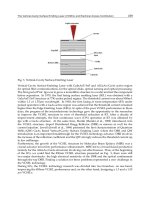
The block diagram of a typical MIMO 2×2 is shown in Fig. 1.


Fig. 1. General architecture of a MIMO 2×2.
where 

, 

are the input (transmitted) signals of time slot 1 in locations  and ,
respectively. 


, 


are associated input signals of time slot 2.
It is assumed that the channel coherence bandwidth is larger than the transmitted signal
bandwidth so that the channel can be considered as narrowband or flat fading. Furthermore,
the channel is assumed to be stationary during the communication process of a block.
Hence, by assuming the block Rayleigh fading model for flat MIMO channels, the channel
response is fixed within one block and changes from one block to another one randomly.
During the training period, the received signal in such a system can be written as (1)
MIMO Systems, Theory and Applications

74
. (1)
where ,  and  are the complex 

-vector of received signals on the 

receive antennas,
the possibly complex 

-vector of transmitted signals on the 

transmit antennas, and the
complex 

-vector of additive receiver noise, respectively. The elements of the noise matrix
are independent and identically distributed (i.i.d.) complex Gaussian random variables with
zero-mean and 


variance, and the correlation matrix of  is then given by (Ma et al., 2005):




.

 


.


.


(2)
where (.)
H
is reserved for the matrix hermitian, . is the mathematical expectation, and 



denotes the 



identity matrix. 

is the number of transmitted training symbols by
each transmitter antenna. The matrix  in the model (1) is the 



matrix of complex
fading coefficients. The ,-th element of the matrix  denoted by 
,
represents the
fading coefficient value between the -th receiver antenna and the -th transmitter antenna.
Here, it is assumed that the MIMO system has equal transmit and receive antennas.
The elements of  and noise are independent of each other. In order to estimate the channel
matrix, it is required that 

P
 N
T
training symbols are transmitted by each transmitter
antenna. The function of a channel estimation algorithm is to recover the channel matrix 
based on the knowledge of  and  (Shirvani Moghaddam & Saremi, 2010).
As depicted in Fig. 1, output (received) signals in locations  and  are as follow:








.



.







.




.








.




.










.





.








(3)
where 

,

are the output signals of time slot 1 in locations  and , respectively. 


,



are associated output signals of time slot 2. 

,

,


,



are independent Additive White
Gaussian Noises (AWGN). In (Alamouti, 1998), Alamouti proposed the first space-time
coding for a MIMO 2×2 system. The proposed matrix is as follow:
S=










 (4)
which means that in the first time slot, 

and 

will be sent and in the second one, 


and



will be transmitted. Following equations can be used to decoding process:







.



.





.



.







.




.





.



.


(5)
This kind of coding is used in this research. Simulation results show its great effect on the
performance of the channel estimators in both TBCE and SBCE-ML schemes.
3. Channel estimators
As illustrated in Table 1, there are many algorithms to estimate the channel response from
training sequence. As shown in introduction and also (Leus & Von Der Veen, 2005: Murthy
et al., 2006), LS, LMMSE, ML, and MAP are the famous and more applicable estimators. In
this investigation, perfect estimator (inverse matrix) is a proper reference to compare the
Joint LS Estimation and ML Detection for Flat Fading MIMO Channels
75
estimators. This reference method offers minimum BER in the case of a Rayleigh flat fading
MIMO channel or AWGN.

Channel Estimator Estimation Formula
Perfect



.


LS




.

.

.
LMMSE





.




.

.

.

ML




.

.

.

.

.
MAP




.


.



.

.



.
Table 1. Different Channel Estimators
where .

is reserved for the matrix inverse, 

and 

denote channel and noise
covariances, respectively.
3.1 Perfect estimator
Perfect estimator is the simplest algorithm to estimate the channel matrix. By setting the
noise equal to zero in (1), the perfect approach estimates the channel matrix as


.

(6)
Using equation (6), sub-channel responses are simply obtained by
























.








.











.
















.








.











.














.











.













.











.


(7)
Substituting (7) back into noise-free version of (3), input signals can be expressed as















.



.



.




.



.









.



.



.



.











.




.



.




.



.












.



.




.



.

(8)
where 

,


are the estimated input signals of time slot 1 in locations  and , and



,


are associated estimated input signals of time slot 2, respectively.
MIMO Systems, Theory and Applications
76
3.2 LS estimator
Considering (1), LS estimator finds 

so that .

. LS Algorithm, minimizes the
Euclidian distance of .

. For this minimization we do following steps:

.






.





.

.






.



.

.




..



.




.

. (9)
By differentiating (9) with respect to 

and setting the result equal to zero, it is obtained
that 

should satisfy the equation (10)
2

..

2

.0

..



. (10)
Finally, the LS channel estimation algorithm is based on (11)


 

.

.


. (11)
3.3 LMMSE estimator
For linear model (1), the MMSE and LMMSE estimators are identical. So, let us minimize the
estimation MSE of . It can be expressed in the following form:


min







(12)
Assuming 



0 and noise is AWGN, we can obtain that (12) will be minimized as


 


.





.

.

. (13)
Comparing (13) and (11), it is obvious that




 


.

.

. (14)
(14) shows that LMMSE needs to find an additional term compared to LS estimator. This
term depends on previous data and introduces more computational complexity.
3.4 ML estimator
To identify  from (1), the ML approach maximizes (15)


 max





|


(15)
where 


|


is the conditional probability of received signal respect to channel response. It
is given that the ML channel estimator (15) yields


 

.

.

.

.

. (16)
3.5 MAP estimator
In order to estimate the channel response, in addition training bits, MAP estimator needs to
find channel covariance as well as noise covariance. MAP channel estimate is in accordance
with previous conditional probability 



|
,

. MAP channel estimate can be found by
solving the following equation:




|
,



|


0 (17)
Joint LS Estimation and ML Detection for Flat Fading MIMO Channels
77
By using the Bay’s identity (18) and solving the equation (17), MAP channel estimate can be
found as (19)



|
,






|
,

.

,




|


(18)


 

.


.



.


.


. (19)
4. Simulation results of TBCE
In order to compare the performance of LS, LMMSE, ML, and MAP estimators in TBCE for
MIMO channels, three cases, MIMO 2×2 without coding, MIMO 4×4, and Alamouti coded
MIMO 2×2 are simulated. Simulation results show the performance of different estimators
in terms of three metrics (BER, SER, and required processing time). For the sake of
simplicity and without loss of generality, we assume Rayleigh flat fading MIMO channel
with AWGN, 4QAM modulation, 8 training bits for MIMO 2×2 (



2) and 32 bits
for MIMO 4×4 (



4) which are generated randomly and followed by 400 data bits.
It is notable that when each point in our figures is obtained by averaging over 1000
independent simulation runs, the numerical and analytical results are almost identical.
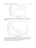
Fig. 2 shows the BER as well as SER of different estimators in the case of TBCE. As depicted,
LS estimator has the better peformace (Lower BER and SER) rather than LMMSE, ML and
MAP estimators and its performance is close to the perfect one.


Fig. 2. Performance metrics (BER, SER) versus SNR for a MIMO 2×2 (TBCE).
As shown in Fig. 3, increasing the number of transmit antennas leads to increase the
performance estimators, but it is highlighted in LS. It means, the performance of LS

algorithm in a MIMO 4×4 system is improved respect to MIMO 2×2. As before, increasing
the SNR is the reason for decreasing BER and SER of all estimators but it is more effective
for LS one.
The BER and SER of TBCE versus SNR for various channel estimators in the case of MIMO
2×2 with Alamouti coding, are shown in Fig. 4. Comparing Fig. 4 and Fig. 2, it is observed
that the BER and SER of all estimators are decreased using Alamouti coding especially at
low SNRs.
Considering the processing time of TBCE equipped with prefect estimator equal to 100, Fig.
5 shows the processing time for other estimators respect to the perfect one. As expected,
minimum processing time belongs to LS estimator.
MIMO Systems, Theory and Applications
78

Fig. 3. Performance metrics (BER, SER) versus SNR for a MIMO 4×4 (TBCE).



Fig. 4. Performance metrics (BER, SER) versus SNR for an Alamouti coded MIMO 2×2 (TBCE).
5. Simulation results of SBCE
For pure TBCE schemes, a long training is necessary in order to obtain a reliable MIMO
channel estimate which reduces the system bandwidth efficiency considerably. SBCE-ML
schemes require less computational complexity than blind methods and fewer training
symbols than training-based methods, making them attractive for practical implementation.
TBCE algorithms use only the training sequences to perform channel estimation, while a
SBCE algorithm takes the data symbols also into account. Since the data symbols are
practically unknown, before they can be used for channel estimation, the receiver has to
perform detection in advance. Thus, the task of channel estimation changes into joint
estimation of channel and data symbols.
By refining the channel estimate and the data decisions in a recursive manner, considerable
performance gain can be achieved step by step. As depicted in Fig. 6, in an iterative

structure, output of estimator is applied to detector for detecting data bits and also output of
detector is applied to the estimator as virtual bits and to estimate the channel again. This
iterative procedure runs until a criterion is achieved [Shirvani Moghaddam & Saremi, 2010].
For example, difference of estimation for two successive iterations is lower than a level. LS,
LMMSE, ML and MAP estimators may be used in estimation part but ML detector is more
attractive in semi-blind joint estimation and detection schemes. In the first step, channel
response is estimated considering short training bits. Then, by using the ML detector,
symbols are detected according to (20):



argmin



  .




 (20)
Joint LS Estimation and ML Detection for Flat Fading MIMO Channels
79

Fig. 5. Relative processing time of different estimators with respect to perfect one in a
MIMO 2×2 (TBCE).


Fig. 6. Iterative structure of channel estimation and data detection in SBCE.
where 



is used for detecting 

and previous detected data is the virtual training
sequence to next estimation. ||.||

denotes the Frobenius norm. This process will be
continued until (21) be satisfied.

,
,
,

,
,
,
 (21)
The proposed method can be summarized as follow:
1. 0: 



    

;
2.   1;
.  
. 
3.  2  

,
,
,

,1
,
,1

In the next subsections, simulation results of SBCE-ML method for a Rayleigh flat fading
MIMO system in three cases, MIMO 2×2 (with and without Alamouti coding) and MIMO
4×4 are presented. For this type of channel estimation, 8 and 32 training bits are used for
MIMO 2×2 and MIMO 4×4, respectively followed by 40000 data bits. simulation results of
SBCE scheme are presented to find the efficient estimator with good performance (BER as
well as SER) and lower processing time.
100
71.4
80
81 81
Perfect LS LMMSE ML MAP
TBCE
MIMO Systems, Theory and Applications
80
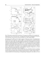
Fig. 7 illustrates the BER as well as SER of SBCE-ML using various estimators versus
different SNR for a Rayleigh flat fading MIMO 2×2 channel. It is obvious that, increasing
SNR is the reason for decreasing both BER and SER. As depicted, not only the performance
of LS algorithm is better than other estimators but also is close to the perfect one.



Fig. 7. Performance metrics (BER, SER) versus SNR for a MIMO 2×2 (SBCE-ML).

Increasing the number of transmit antennas leads to decreasing the performance estimators,
except LS. As shown in Fig. 8, the performance of LS algorithm in a MIMO 4×4 system is
improved respect to MIMO 2×2. In the other hand, a power gain or SNR improvement will
be achieved. For example in SBCE-ML, transmitting power will be saved about 3 dB, if BER
equals to 0.3.


Fig. 8. Performance metrics (BER, SER) versus SNR for a MIMO 4×4 (SBCE-ML).
The BER and SER of SBCE-ML method versus SNR for various channel estimators in the
case of MIMO 2×2 with Alamouti coding, are shown in Fig. 9. it is observed that the LS
estimator outperforms the other estimators especially at low SNRs.


Fig. 9. Performance metrics (BER, SER) versus SNR for an Alamouti coded MIMO 2×2
(SBCE-ML).
Joint LS Estimation and ML Detection for Flat Fading MIMO Channels
81
Fig. 10 shows the processing time for different estimators (LS, LMMSE, ML, MAP) with
respect to the perfect estimator in SBCE-ML scheme. In this figure, required time for perfect
one is considered as 100 and other estimators‘ processing time is evaluated based on the
perfect one. It is obvious that minimum processing time belongs to LS estimator.


Fig. 10. Relative processing time of different estimators with respect to perfect one in a
MIMO 2×2 (SBCE).
6. Comparison of LS-based TBCE and joint LS-estimation & ML-detection
SBCE
Simulation results of TBCE and SBCE-ML methods show that the required processing time
and both BER and SER of LS estimator compared with other estimators is much better. In
this section by focusing on LS estimator, LS-based TBCE and LS-based SBCE-ML are

compared in a MIMO 2 × 2 (with and without Alamouti coding) and a MIMO 4×4, for
different SNRs based on BER, SER, required channel estimation processing time and relative
length of training bits.
Fig. 11 indicates the BER and SER metrics of LS-based TBCE and LS-based SBCE-ML
schemes for different SNRs. As shown, for both TBCE and SBCE-ML methods, increasing
SNR is the reason for decreasing both BER and SER. As depicted in this figure, SBCE-ML
offers a bit better performance rather than TBCE.

Fig. 11. Performance metrics (BER, SER) of LS-based TBCE and SBCE-ML schemes in
different SNRs for a MIMO 2×2.
100
89
95
95.8
96.4
Perfect LS LMMSE ML MAP
SBCE-ML
MIMO Systems, Theory and Applications
82
As shown in Fig. 12, the performance of both LS-based TBCE and SBCE-ML schemes in a
MIMO 4×4 system is improved respect to MIMO 2×2. In the other hand, a power gain or
SNR improvement will be achieved. For example in SBCE-ML, transmitting power will be
saved about 3 dB, if BER equals to 0.3. In TBCE method, for BER equals to 0.2, transmitting
power will be saved about 0.5 dB. It is worthwhile to note that the excess of transmit or/and
receive antennas in MIMO systems leads to a higher capacity.


Fig. 12. Performance metrics (BER, SER) of LS-based TBCE and SBCE-ML schemes in
different SNRs for a MIMO 4×4.
The BER and SER of both LS-based TBCE and SBCE-ML schemes versus SNR in the case of

MIMO 2×2 with Alamouti coding, are shown in Fig. 13. As shown in this figure, when SNR
equals to 0.25 dB, BER is 0.0130 for SBCE-ML and 0.0386 for TBCE. It means 3 times better
performance in lowest SNRs for SBCE-ML method rather than TBCE one. At higher SNRs,
the performance of LS estimator in both channel estimation schemes is analogous.
By considering the required processing time of LS-based TBCE and SBCE-ML schemes
rlated to prefect estimator, Fig. 14 shows that SBCE-ML method needs 25 percent more
processing time to estimate the channel than TBCE method. It is due to joint LS estimation
and ML detection of SBCE method.
Fig. 15, 16 show the required training sequences in each frame of data for TBCE and SBCE-
ML schemes, respectively. As depicted in Fig. 15, in TBCE method, transmitter sends 8
training bits before 400 information bits in each burst for a MIMO 2×2 system and 32 bits for
a MIMO 4×4 system. Figure 16, illustrates the required number of training and information
bits in SBCE-ML method for both MIMO 2×2 and MIMO 4×4. Considering the same training
bits, 400 information bits in the case of TBCE method are changed to 40000 bits in SBCE-ML.
As mentioned before, TBCE method needs more bits to estimate the channel because
training sequences should be transmitted periodically. On the other word, SBCE-ML



Fig. 13. Performance metrics (BER, SER) of LS-based TBCE and SBCE-ML schemes in
different SNRs for an Alamouti coded MIMO 2×2.
Joint LS Estimation and ML Detection for Flat Fading MIMO Channels
83


Fig. 14. Relative processing time of LS-based TBCE and SBCE-ML schemes in a MIMO 2×2.


Fig. 15. The burst of LS-based TBCE. A) MIMO 2×2, B) MIMO 4×4.

Fig. 16. The burst of LS-based SBCE-ML. A) MIMO 2×2, B) MIMO 4×4.
method needs to transmit just one training sequence. Therefore, redundancies of TBCE
method are 2% and 8% for MIMO 2×2 and MIMO 4×4 systems, respectively. In the case of
SBCE-ML method, redundancies are 0.02% and 0.08%, respectively. It means 100 times
lower training bits for SBCE-ML respect to TBCE.
7. Conclusion
MIMO systems play a vital role in fourth generation wireless systems to provide advanced
data rate. In order to attain the advantages of MIMO systems, it is necessary that the receiver
and/or transmitter have access CSI. The time-varying nature of the channel typically requires
the use of frequent channel retraining, which in turn increases the data overhead due to
training signals, thus reducing the system’s overall spectral efficiency. Hence, effective channel
estimation algorithms are needed to guarantee the performance of communication.
In this chapter, training based as well as semi-blind channel estimation schemes in Rayleigh
flat fading MIMO systems are investigated. After introducing LS, LMMSE, ML and MAP
estimators, they are simulated in a Rayleigh flat fading MIMO channel considering AWGN.
Simulation results show that LS estimator is the best choice in both TBCE and SBCE-ML
schemes. This selection is due to faster processing and lower BER as well as SER of LS
estimator with respect to other estimators. In addition, it is illustrated that when the number
71.4
89
0
20
40
60
80
100
TBCE SBCE-ML