Mpeg 7 audio and beyond audio content indexing and retrieval phần 5 ppt
Bạn đang xem bản rút gọn của tài liệu. Xem và tải ngay bản đầy đủ của tài liệu tại đây (462.14 KB, 31 trang )
104 4 SPOKEN CONTENT
In this chapter we use the well defined MPEG-7 Spoken Content description
standard as an example to illustrate challenges in this domain. The audio part
of MPEG-7 contains a SpokenContent high-level tool targeted at spoken data
management applications. The MPEG-7 SpokenContent tool provides a stan-
dardized representation of an ASR output, i.e. of the semantic information (the
spoken content) extracted by an ASR system from a spoken signal. The Spo-
kenContent description attempts to be memory efficient and flexible enough to
make currently unforeseen applications possible in the future. It consists of a
compact representation of multiple word and/or sub-word hypotheses produced
by an ASR engine. It also includes a header that contains information about the
recognizer itself and the speaker’s identity.
How the SpokenContent description should be extracted and used is not part of
the standard. However, this chapter begins with a short introduction to ASR sys-
tems. The structure of the MPEG-7 SpokenContent description itself is presented
in detail in the second section. The third section deals with the main field of appli-
cation of the SpokenContent tool, called spoken document retrieval (SDR), which
aims at retrieving information in speech signals based on their extracted contents.
The contribution of the MPEG-7 SpokenContent tool to the standardization and
development of future SDR applications is discussed at the end of the chapter.
4.2 AUTOMATIC SPEECH RECOGNITION
The MPEG-7 SpokenContent description is a normalized representation of the
output of an ASR system. A detailed presentation of the ASR field is beyond the
scope of this book. This section provides a basic overview of the main speech
recognition principles. A large amount of literature has been published on the
subject in the past decades. An excellent overview on ASR is given in (Rabiner
and Juang, 1993).
Although the extraction of the MPEG-7 SpokenContent description is non-
normative, this introduction is restrained to the case of ASR based on hidden
Markov models, which is by far the most commonly used approach.
4.2.1 Basic Principles
Figure 4.1 gives a schematic description of an ASR process. Basically, it consists
in two main steps:
1. Acoustic analysis. Speech recognition does not directly process the speech
waveforms. A parametric representation X (called acoustic observation)of
speech acoustic properties is extracted from the input signal A.
2. Decoding. The acoustic observation X is matched against a set of predefined
acoustic models. Each model represents one of the symbols used by the system
4.2 AUTOMATIC SPEECH RECOGNITION 105
Sequence of
Recognized Symbols
W
Acoustic
Analysis
Speech Signal
A
Decoding
Acoustic
Parameters
Recognition System
X
Acoustic
Models
Figure 4.1 Schema of an ASR system
for describing the spoken language of the application (e.g. words, syllables
or phonemes). The best scoring models determine the output sequence of
symbols.
The main principles and definitions related to the acoustic analysis and decod-
ing modules are briefly introduced in the following.
4.2.1.1 Acoustic Analysis
The acoustic observation X results from a time–frequency analysis of the input
speech signal A. The main steps of this process are:
1. The analogue signal is first digitized. The sampling rate depends on the par-
ticular application requirements. The most common sampling rate is 16 kHz
(one sample every 625 s).
2. A high-pass, also called pre-emphasis, filter is often used to emphasize the
high frequencies.
3. The digital signal is segmented into successive, regularly spaced time intervals
called acoustic frames. Time frames overlap each other. Typically, a frame
duration is between 20 and 40 ms, with an overlap of 50%.
4. Each frame is multiplied by a windowing function (e.g. Hanning).
5. The frequency spectrum of each single frame is obtained through a Fourier
transform.
6. A vector of coefficients x, called an observation vector, is extracted from
the spectrum. It is a compact representation of the spectral properties of the
frame.
Many different types of coefficient vectors have been proposed. The most cur-
rently used ones are based on the frame cepstrum: namely, linear prediction
cepstrum coefficients (LPCCs) and more especially mel-frequency cepstral coef-
ficients (MFCCs) (Angelini et al. 1998; Rabiner and Juang, 1993). Finally, the
106 4 SPOKEN CONTENT
acoustic analysis module delivers a sequence X of observation vectors, X =
x
1
x
2
x
T
, which is input into the decoding process.
4.2.1.2 Decoding
In a probabilistic ASR system, the decoding algorithm aims at determining the
most probable sequence of symbols W knowing the acoustic observation X:
∧
W
= argmax
W
PW X (4.1)
Bayes’ rule gives:
∧
W
= argmax
W
PXWPW
PX
(4.2)
This formula makes two important terms appear in the numerator: PXW and
PW. The estimation of these probabilities is the core of the ASR problem. The
denominator PX is usually discarded since it does not depend on W .
The PXW term is estimated through the acoustic models of the symbols
contained in W . The hidden Markov model (HMM) approach is one of the
most powerful statistical methods for modelling speech signals (Rabiner, 1989).
Nowadays most ASR systems are based on this approach.
A basic example of an HMM topology frequently used to model speech is
depicted in Figure 4.2. This left–right topology consists of different elements:
•
A fixed number of states S
i
.
•
Probability density functions b
i
, associated to each state S
i
. These functions
are defined in the same space of acoustic parameters as the observation vectors
comprising X.
•
Probabilities of transition a
ij
between states S
i
and S
j
. Only transitions with
non-null probabilities are represented in Figure 4.2. When modelling speech,
no backward HMM transitions are allowed in general (left–right models).
These kinds of models allow us to account for the temporal and spectral vari-
ability of speech. A large variety of HMM topologies can be defined, depending
on the nature of the speech unit to be modelled (words, phones, etc.).
Figure 4.2 Example of a left–right HMM
4.2 AUTOMATIC SPEECH RECOGNITION 107
When designing a speech recognition system, an HMM topology is defined
a priori for each of the spoken content symbols in the recognizer’s vocabulary.
The training of model parameters (transition probabilities and probability density
functions) is usually made through a Baum–Welch algorithm (Rabiner and Juang,
1993). It requires a large training corpus of labelled speech material with many
occurrences of each speech unit to be modelled.
Once the recognizer’s HMMs have been trained, acoustic observations can
be matched against them using the Viterbi algorithm, which is based on the
dynamic programming (DP) principle (Rabiner and Juang, 1993).
The result of a Viterbi decoding algorithm is depicted in Figure 4.3. In this
example, we suppose that sequence W just consists of one symbol (e.g. one
word) and that the five-state HMM
W
depicted in Figure 4.2 models that word.
An acoustic observation X consisting of six acoustic vectors is matched against
W
. The Viterbi algorithm aims at determining the sequence of HMM states that
best matches the sequence of acoustic vectors, called the best alignment. This is
done by computing sequentially a likelihood score along every authorized paths
in the DP grid depicted in Figure 4.3. The authorized trajectories within the grid
are determined by the set of HMM transitions. An example of an authorized path
is represented in Figure 4.3 and the corresponding likelihood score is indicated.
Finally, the path with the higher score gives the best Viterbi alignment.
The likelihood score of the best Viterbi alignment is generally used to approx-
imate PXW in the decision rule of Equation (4.2). The value corresponding
to the best recognition hypothesis – that is, the estimation of PX
W – is called
the acoustic score of X.
The second term in the numerator of Equation (4.2) is the probability PW
of a particular sequence of symbols W . It is estimated by means of a stochastic
language model (LM). An LM models the syntactic rules (in the case of words)
HMM
for word W
λ
w
S
5
S
4
S
3
S
2
S
1
x
1
x
2
x
3
x
4
x
5
x
6
(
*
)
(
*
) Likelihood Score = b
1
(x
1
).a
13
.b
3
(x
2
).a
34
.b
4
(x
3
).a
44
.b
4
(x
4
).a
45
.b
5
(x
5
).a
55
.b
5
(x
6
)
Acoustic Observation X
Figure 4.3 Result of a Viterbi decoding
108 4 SPOKEN CONTENT
or phonotactic rules (in the case of phonetic symbols) of a given language, i.e.
the rules giving the permitted sequences of symbols for that language.
The acoustic scores and LM scores are not computed separately. Both are
integrated in the same process: the LM is used to constrain the possible sequences
of HMM units during the global Viterbi decoding. At the end of the decoding
process, the sequence of models yielding the best accumulated LM and likelihood
score gives the output transcription of the input signal. Each symbol comprising
the transcription corresponds to an alignment with a sub-sequence of the input
acoustic observation X and is attributed an acoustic score.
4.2.2 Types of Speech Recognition Systems
The HMM framework can model any kind of speech units (words, phones, etc.)
allowing us to design systems with diverse degrees of complexity (Rabiner,
1993). The main types of ASR systems are listed below.
4.2.2.1 Connected Word Recognition
Connected word recognition systems are based on a fixed syntactic network,
which strongly restrains the authorized sequences of output symbols. No stochas-
tic language model is required. This type of recognition system is only used for
very simple applications based on a small lexicon (e.g. digit sequence recogni-
tion for vocal dialling interfaces, telephone directory, etc.) and is generally not
adequate for more complex transcription tasks.
An example of a syntactic network is depicted in Figure 4.4, which represents
the basic grammar of a connected digit recognition system (with a backward
transition to permit the repetition of digits).
Figure 4.4 Connected digit recognition with (a) word modelling and (b) flexible
modelling
4.2 AUTOMATIC SPEECH RECOGNITION 109
Figure 4.4 also illustrates two modelling approaches. The first one (a) consists
of modelling each vocabulary word with a dedicated HMM. The second (b) is a
sub-lexical approach where each word model is formed from the concatenation
of sub-lexical HMMs, according to the word’s canonical transcription (a phonetic
transcription in the example of Figure 4.4). This last method, called flexible
modelling, has several advantages:
•
Only a few models have to be trained. The lexicon of symbols necessary to
describe words has a fixed and limited size (e.g. around 40 phonetic units to
describe a given language).
•
As a consequence, the required storage capacity is also limited.
•
Any word with its different pronunciation variants can be easily modelled.
•
New words can be added to the vocabulary of a given application without
requiring any additional training effort.
Word modelling is only appropriate with the simplest recognition systems, such
as the one depicted in Figure 4.4 for instance. When the vocabulary gets too
large, as in the case of large-vocabulary continuous recognition addressed in
the next section, word modelling becomes clearly impracticable and the flexible
approach is mandatory.
4.2.2.2 Large-Vocabulary Continuous Speech Recognition
Large-vocabulary continuous speech recognition (LVCSR) is a speech-to-text
approach, targeted at the automatic word transcription of the input speech signal.
This requires a huge word lexicon. As mentioned in the previous section, words
are modelled by the concatenation of sub-lexical HMMs in that case. This means
that a complete pronunciation dictionary is available to provide the sub-lexical
transcription of every vocabulary word.
Recognizing and understanding natural speech also requires the training of a
complex language model which defines the rules that determine what sequences
of words are grammatically well formed and meaningful. These rules are intro-
duced in the decoding process by applying stochastic constraints on the permitted
sequences of words.
As mentioned before (see Equation 4.2), the goal of stochastic language models
is the estimation of the probability PW of a sequence of words W . This not only
makes speech recognition more accurate, but also helps to constrain the search
space for speech recognition by discarding the less probable word sequences.
There exist many different types of LMs (Jelinek, 1998). The most widely
used are the so-called n-gram models, where PW is estimated based on
probabilities Pw
i
w
i−n+1
w
i−n+2
w
i−1
that a word w
i
occurs after a sub-
sequence of n−1 words w
i−n+1
w
i−n+2
w
i−1
. For instance, an LM where
the probability of a word only depends on the previous one Pw
i
w
i−1
is
110 4 SPOKEN CONTENT
called a bigram. Similarly, a trigram takes the two previous words into account
Pw
i
w
i−2
w
i−1
.
Whatever the type of LM, its training requires large amounts of texts or
spoken document transcriptions so that most of the possible word successions
are observed (e.g. possible word pairs for a bigram LM). Smoothing methods are
usually applied to tackle the problem of data sparseness (Katz, 1987). A language
model is dependent on the topics addressed in the training material. That means
that processing spoken documents dealing with a completely different topic could
lead to a lower word recognition accuracy.
The main problem of LVCSR is the occurrence of out-of-vocabulary (OOV)
words, since it is not possible to define a recognition vocabulary comprising
every possible word that can be spoken in a given language. Proper names are
particularly problematic since new ones regularly appear in the course of time
(e.g. in broadcast news). They often carry a lot of useful semantic information
that is lost at the end of the decoding process. In the output transcription, an OOV
word is usually substituted by a vocabulary word or a sequence of vocabulary
words that is acoustically close to it.
4.2.2.3 Automatic Phonetic Transcription
The goal of phonetic recognition systems is to provide full phonetic transcriptions
of spoken documents, independently of any lexical knowledge. The lexicon is
restrained to the set of phone units necessary to describe the sounds of a given
language (e.g. around 40 phones for English).
As before, a stochastic language model is needed to prevent the generation
of less probable phone sequences (Ng et al., 2000). Generally, the recognizer’s
grammar is defined by a phone loop, where all phone HMMs are connected
with each other according to the phone transition probabilities specified in the
phone LM. Most systems use a simple stochastic phone–bigram language model,
defined by the set of probabilities P
j
i
that phone
j
follows phone
i
(James, 1995; Ng and Zue, 2000b).
Other, more refined phonetic recognition systems have been proposed. The
extraction of phones by means of the SUMMIT system (Glass et al., 1996)
developed at MIT,
1
adopts a probabilistic segment-based approach that differs
from conventional frame-based HMM approaches. In segment-based approaches,
the basic speech units are variable in length and much longer in comparison
with frame-based methods. The SUMMIT system uses an “acoustic segmenta-
tion” algorithm (Glass and Zue, 1988) to produce the segmentation hypotheses.
Segment boundaries are hypothesized at locations of large spectral change. The
boundaries are then fully interconnected to form a network of possible segmen-
tations on which the recognition search is performed.
1
Massachusetts Institute of Technology.
4.2 AUTOMATIC SPEECH RECOGNITION 111
Another approach to word-independent sub-lexical recognition is to train
HMMs for other types of sub-lexical units, such as syllables (Larson and
Eickeler, 2003). But in any case, the major problem of sub-lexical recognition
is the high rate of recognition errors in the output sequences.
4.2.2.4 Keyword Spotting
Keyword spotting is a particular type of ASR. It consists of detecting the occur-
rences of isolated words, called keywords, within the speech stream (Wilpon
et al., 1990). The target words are taken from a restrained, predefined list of
keywords (the keyword vocabulary).
The main problem with keyword spotting systems is the modeling of irrelevant
speech between keywords by means of so-called filler models. Different sorts of
filler models have been proposed. A first approach consists of training different
specific HMMs for distinct “non-keyword” events: silence, environmental noise,
OOV speech, etc. (Wilpon et al., 1990). Another, more flexible solution is
to model non-keyword speech by means of an unconstrained phone loop that
recognizes, as in the case of a phonetic transcriber, phonetic sequences without
any lexical constraint (Rose, 1995). Finally, a keyword spotting decoder consists
of a set of keyword HMMs looped with one or several filler models.
During the decoding process, a predefined threshold is set on the acoustic score
of each keyword candidate. Words with scores above the threshold are considered
true hits, while those with scores below are considered false alarms and ignored.
Choosing the appropriate threshold is a trade-off between the number of type
I (missed words) and type II (false alarms) errors, with the usual problem that
reducing one increases the other. The performance of keyword spotting systems
is determined by the trade-offs it is able to achieve. Generally, the desired trade-
off is chosen on a performance curve plotting the false alarm rate vs. the missed
word rate. This curve is obtained by measuring both error rates on a test corpus
when varying the decision threshold.
4.2.3 Recognition Results
This section presents the different output formats of most ASR systems and
gives the definition of recognition error rates.
4.2.3.1 Output Format
As mentioned above, the decoding process yields the best scoring sequence
of symbols. A speech recognizer can also output the recognized hypotheses in
several other ways. A single recognition hypothesis is sufficient for the most basic
systems (connected word recognition), but when the recognition task is more
complex, particularly for systems using an LM, the most probable transcription
112 4 SPOKEN CONTENT
usually contains many errors. In this case, it is necessary to deliver a series of
alternative recognition hypotheses on which further post-processing operations
can be performed. The recognition alternatives to the best hypothesis can be
represented in two ways:
•
An N-best list , where the N most probable transcriptions are ranked according
to their respective scores.
•
A lattice, i.e. a graph whose different paths represent different possible tran-
scriptions.
Figure 4.5 depicts the two possible representations of the transcription alterna-
tives delivered by a recognizer (A, B, C and D represent recognized symbols).
A lattice offers a more compact representation of the transcription alternatives.
It consists of an oriented graph in which nodes represent time points between the
beginning T
start
and the end T
end
of the speech signal. The edges correspond
to recognition hypotheses (e.g. words or phones). Each one is assigned the label
and the likelihood score of the hypothesis it represents along with a transition
probability (derived from the LM score). Such a graph can be seen as a reduced
representation of the initial search space. It can be easily post-processed with an
A
∗
algorithm (Paul, 1992), in order to extract a list of N -best transcriptions.
4.2.3.2 Performance Measurements
The efficiency of an ASR system is generally measured based on the 1-best tran-
scriptions it delivers. The transcriptions extracted from an evaluation collection
of spoken documents are compared with reference transcriptions. By comparing
reference and hypothesized sequences, the occurrences of three types or errors
are usually counted:
Figure 4.5 Two different representations of the output of a speech recognizer. Part (a)
depicts a list of N -best transcriptions, and part (b) a word lattice
4.3 MPEG-7 SPOKENCONTENT DESCRIPTION 113
•
Substitution errors, when a symbol in the reference transcription was substi-
tuted with a different one in the recognized transcription.
•
Deletion errors, when a reference symbol has been omitted in the recognized
transcription.
•
Insertion errors, when the system recognized a symbol not contained in the
reference transcription.
Two different measures of recognition performance are usually computed based
on these error counts. The first is the recognition error rate:
Error Rate =
# Substitution + #Insertion + #Deletion
# Reference Symbols
(4.3)
where #Substitution,#Insertion and #Deletion respectively denote the numbers
of substitution, insertion and deletion occurrences observed when comparing the
recognized transcriptions with the reference. #Reference Symbols is the number
of symbols (e.g. words) in the reference transcriptions. The second measure is
the recognition accuracy:
Accuracy =
#Correct − #Insertion
# Reference Symbols
(4.4)
where #Correct denotes the number of symbols correctly recognized. Only one
performance measure is generally mentioned since:
Accuracy + Error Rate = 100% (4.5)
The best performing LVCSR systems can achieve word recognition accuracies
greater than 90% under certain conditions (speech captured in a clean acoustic
environment). Sub-lexical recognition is a more difficult task because it is syntac-
tically less constrained than LVCSR. As far as phone recognition is concerned,
a typical phone error rate is around 40% with clean speech.
4.3 MPEG-7 SPOKENCONTENT DESCRIPTION
There is a large variety of ASR systems. Each system is characterized by a large
number of parameters: spoken language, word and phonetic lexicons, quality
of the material used to train the acoustic models, parameters of the language
models, etc. Consequently, the outputs of two different ASR systems may differ
completely, making retrieval in heterogeneous spoken content databases difficult.
The MPEG-7 SpokenContent high-level description aims at standardizing the
representation of ASR outputs, in order to make interoperability possible. This
is achieved independently of the peculiarities of the recognition engines used to
extract spoken content.
114 4 SPOKEN CONTENT
4.3.1 General Structure
Basically, the MPEG-7 SpokenContent tool defines a standardized description
of the lattices delivered by a recognizer. Figure 4.6 is an illustration of what
an MPEG-7 SpokenContent description of the speech excerpt “film on Berlin”
could look like. Figure 4.6 shows a simple lattice structure where small circles
represent lattice nodes. Each link between nodes is associated with a recognition
hypothesis, a probability derived from the language model, and the acoustic score
delivered by the ASR system for the corresponding hypothesis. The standard
defines two types of lattice links: word type and phone type. An MPEG-7 lattice
can thus be a word-only graph, a phone-only graph or combine word and phone
hypotheses in the same graph as depicted in the example of Figure 4.6.
The MPEG-7 a SpokenContent description consists of two distinct elements:
a SpokenContentHeader and a SpokenContentLattice. The SpokenContentLattice
represents the actual decoding produced by an ASR engine (a lattice structure
such as the one depicted in Figure 4.6). The SpokenContentHeader contains
some metadata information that can be shared by different lattices, such as the
recognition lexicons of the ASR systems used for extraction or the speaker
identity. The SpokenContentHeader and SpokenContentLattice descriptions are
interrelated by means of specific MPEG-7 linking mechanisms that are beyond
the scope of this book (Lindsay et al., 2000).
4.3.2 SpokenContentHeader
The SpokenContentHeader contains some header information that can be shared
by several SpokenContentLattice descriptions. It consists of five types of
metadata:
•
WordLexicon: a list of words. A header may contain several word lexicons.
•
PhoneLexicon: a list of phones. A header may contain several phone lexicons.
Figure 4.6 MPEG-7 SpokenContent description of an input spoken signal “film on
Berlin”
4.3 MPEG-7 SPOKENCONTENT DESCRIPTION 115
•
ConfusionInfo: a data structure enclosing some phone confusion information.
Although separate, the confusion information must map onto the phone lexicon
with which it is associated via the SpeakerInfo descriptor.
•
DescriptionMetadata: information about the extraction process used to gener-
ate the lattices. In particular, this data structure can store the name and settings
of the speech recognition engine used for lattice extraction.
•
SpeakerInfo: information about the persons speaking in the original audio
signals, along with other information about their associated lattices.
These descriptors are mostly detailed in the following sections.
4.3.2.1 WordLexicon
A WordLexicon is a list of words, generally the vocabulary of a word-based
recognizer. Each entry of the lexicon is an identifier (generally its orthographic
representation) representing a word. A WordLexicon consists of the following
elements:
•
phoneticAlphabet: is the name of an encoding scheme for phonetic symbols. It
is only needed if phonetic representations are used (see below). The possible
values of this attribute are indicated in the PhoneLexicon section.
•
NumOfOriginalEntries: is the original size of the lexicon. In the case of a
word lexicon, this should be the number of words originally known to the
ASR system.
•
A series of Token elements: each one stores an entry of the lexicon.
Each Token entry is made up of the following elements:
•
Word: a string that defines the label corresponding to the word entry. The
Word string must not contain white-space characters.
•
representation: an optional attribute that describes the type of representation
of the lexicon entry. Two values are possible: orthographic (the word is
represented by its normal orthographic spelling) or nonorthographic (the word
is represented by another kind of identifier). A non-orthographic representation
may be a phoneme string corresponding to the pronunciation of the entry,
encoded according to the phoneticAlphabet attribute.
•
linguisticUnit: an optional attribute that indicates the type of the linguistic unit
corresponding to the entry.
The WordLexicon was originally designed to store an ASR word vocabu-
lary. The linguisticUnit attribute was introduced also to allow the definition
116 4 SPOKEN CONTENT
of other types of lexicons. The possible values for the linguisticUnit attribute
are:
•
word: the default value.
•
syllable: a sub-word unit (generally comprising two or three phonetic units)
derived from pronunciation considerations.
•
morpheme: a sub-word unit bearing a semantic meaning in itself (e.g. the
“psycho” part of word “psychology”).
•
stem: a prefix common to a family of words (e.g. “hous” for “house”, “houses”,
“housing”, etc.).
•
affix: a word segment that needs to be added to a stem to form a word.
•
component: a constituent part of a compound word that can be useful for
compounding languages like German.
•
nonspeech: a non-linguistic noise.
•
phrase: a sequence of words, taken as a whole.
•
other: another linguistic unit defined for a specific application.
The possibility to define non-word lexical entries is very useful. As will be later
explained, some spoken content retrieval approaches exploit the above-mentioned
linguistic units. The extraction of these units from speech can be done in two ways:
•
A word-based ASR system extracts a word lattice. A post- processing of
word labels (for instance, a word-to-syllable transcription algorithm based on
pronunciation rules) extracts the desired units.
•
The ASR system is based on a non-word lexicon. It extracts the desired linguistic
information directly from speech. It could be, for instance, a syllable recognizer,
based on a complete syllable vocabulary defined for a given language.
In the MPEG-7 SpokenContent standard, the case of phonetic units is handled
separately with dedicated description tools.
4.3.2.2 PhoneLexicon
A PhoneLexicon is a list of phones representing the set of phonetic units (basic
sounds) used to describe a given language. Each entry of the lexicon is an
identifier representing a phonetic unit, according to a specific phonetic alphabet.
A WordLexicon consists of the following elements:
•
phoneticAlphabet: is the name of an encoding scheme for phonetic symbols
(see below).
•
NumOfOriginalEntries: is the size of the phonetic lexicon. It depends on the
spoken language (generally around 40 units) and the chosen phonetic alphabet.
•
A series of Token elements: each one stores a Phone string corresponding to an
entry of the lexicon. The Phone strings must not contain white-space characters.
4.3 MPEG-7 SPOKENCONTENT DESCRIPTION 117
The phoneticAlphabet attribute has four possible values:
•
sampa: use of the symbols from the SAMPA alphabet.
1
•
ipaSymbol: use of the symbols from the IPA alphabet.
2
•
ipaNumber: use of the three-digit IPA index.
3
•
other: use of another, application-specific alphabet.
A PhoneLexicon may be associated to one or several ConfusionCount
descriptions.
4.3.2.3 ConfusionInfo
In the SpokenContentHeader description, the ConfusionInfo field actually refer to
a description called ConfusionCount. The ConfusionCount description contains
confusion statistics computed on a given evaluation collection, with a particular
ASR system. Given a spoken document in the collection, these statistics are
calculated by comparing the two following phonetic transcriptions:
•
The reference transcription REF of the document. This results either from
manual annotation or from automatic alignment of the canonical phonetic
transcription of the speech signal. It is supposed to reflect exactly the phonetic
pronunciation of what is spoken in the document.
•
The recognized transcription REC of the document. This results from the
decoding of the speech signal by the ASR engine. Unlike the reference tran-
scription REF, it is corrupted by substitution, insertion and deletion errors.
The confusion statistics are obtained by string alignment of the two transcriptions,
usually by means of a dynamic programming algorithm.
Structure
A ConfusionCount description consists of the following elements:
•
numOfDimensions: the dimensionality of the vectors and matrix in the Con-
fusionCount description. This number must correspond to the size of the
PhoneLexicon to which the data applies.
•
Insertion: a vector (of length numOfDimensions) of counts, being the number
of times a phone was inserted in sequence REC, which is not in REF.
•
Deletion: a vector (of length numOfDimensions) of counts, being the number
of times a phone present in sequence REF was deleted in REC.
1
Speech Assessment Methods Phonetic Alphabet (SAMPA): www.phon.ucl.ac.uk/home/sampa.
2
International Phonetic Association (IPA) Alphabet: />3
IPA Numbers: />118 4 SPOKEN CONTENT
•
Substitution: a square matrix (dimension numOfDimensions) of counts, report-
ing for each phone r in row (REF) the number of times that phone has been
substituted with the phones h in column (REC). The matrix diagonal gives
the number of correct decodings for each phone.
Confusion statistics must be associated to a PhoneLexicon , also provided in the
descriptor’s header. The confusion counts in the above matrix and vectors are
ranked according to the order of appearance of the corresponding phones in the
lexicon.
Usage
We define the substitution count matrix Sub, the insertion and deletion count
vectors Ins and Del respectively and denote the counts in ConfusionCount as
follows:
•
Each element Subr h of the substitution matrix corresponds to the number
of times that a reference phone r of transcription REF was confused with a
hypothesized phone h in the recognized sequence REC. The diagonal elements
Subr r give the number of times a phone r was correctly recognized.
•
Each element Insh of the insertion vector is the number of times that phone
h was inserted in sequence REC when there was nothing in sequence REF at
that point.
•
Each element Delr of the deletion vector is the number of times that phone
r in sequence REF was deleted in sequence REC.
The MPEG-7 confusion statistics are stored as pure counts. To be usable in most
applications, they must be converted into probabilities. The simplest method
is based on the maximum likelihood criterion. According to this method, an
estimation of the probability of confusing phone r as phone h (substitution error)
is obtained by normalizing the confusion count Subr h as follows (Ng and
Zue, 2000):
P
C
r h =
Subr h
Delr +
k
Subr k
≈ Phr (4.6)
The denominator of this ratio represents the total number of occurrences of
phone r in the whole collection of reference transcriptions.
The P
C
matrix that results from the normalization of the confusion count
matrix Sub is usually called the phone confusion matrix (PCM) of the ASR
system. There are many other different ways to calculate such PCMs using
Bayesian or maximum entropy techniques. However, the maximum likelihood
approach is the most straightforward and hence the most commonly used.
4.3 MPEG-7 SPOKENCONTENT DESCRIPTION 119
The deletion and insertion count vectors Del and Ins can be normalized in
the same way. An estimation of the probability of a phone r being deleted is
given by:
P
D
r =
Delr
Delr +
k
Subr k
≈ Pr (4.7)
where is the null symbol, indicating a phone absence.
Similarly, an estimation of the probabilities of a phone h being inserted, given
an insertion took place, is derived from the insertion count vector Ins:
P
I
h =
Insh
k
Insk
≈ Ph (4.8)
The denominator of this ratio represents the total number of insertions in the
whole collection; that is, the number of times any phone appeared in a REC
sequence where there was nothing in the corresponding REF sequence at that
point.
Figure 4.7 gives an example of a phone confusion matrix, along with phone
insertion and deletion vectors. This matrix was obtained with a German phone
recognizer and a collection of German spoken documents.
The estimated probability values P in the matrix and vectors are represented
by grey squares. We used a linear grey scale spanning from white P = 0 to
black P = 1: the darker the square, the higher the P value.
The phone lexicon consists of 41 German phone symbols derived from the
SAMPA phonetic alphabet (Wells, 1997). The blocks along the diagonal group
together phones that belong to the same broad phonetic category. The following
observations can be made from the results in Figure 4.7:
•
The diagonal elements P
C
r r correspond to the higher probability val-
ues. These are estimations of probabilities Prr that phones r are correctly
recognized.
•
Phone confusions are not symmetric. Given two phones i and j, we have
P
C
j i = P
C
i j.
•
Most of the phonetic substitution errors occur between phones that are within
the same broad phonetic class (Halberstadt, 1998).
The phone confusion information can be used in phone-based retrieval systems,
as will be explained later in this chapter.
4.3.2.4 SpeakerInfo
The SpeakerInfo description contains information about a speaker, which may be
shared by several lattices. It effectively contains a Person element representing
120 4 SPOKEN CONTENT
INSERTION VECTOR P
1
(h)
(? = Glottal Stop)
Plosives
Fricatives
Sonorants
Vowels
CONFUSION
MATRIX
P
C
(r, h)
DELETION VECTOR P
D
(r)
REFERENCE PHONE LABELS (r)
RECOGNIZED PHONE LABELS (h)
p
b
t
d
k
g
f
v
s
z
S
C
j
x
h
m
n
N
I
I
r
E
a
O
U
Y
9
i:
e:
E:
a:
o:
u:
y:
2:
aI
aU
OY
@
6
p
b
t
d
k
g
f
v
s
z
S
C
j
x
h
m
n
N
I
I
r
E
a
O
U
Y
9
i:
e:
E:
a:
o:
u:
y:
2:
aI
aU
OY
@
6
?
?
∅
∅
Figure 4.7 Phone confusion matrix of German phones with main phonetic classes
the person who is speaking, but also contains much more information about
lattices, such as indexes and references to confusion information and lexicons.
A SpeakerInfo consists of these elements:
•
Person: is the name (or any other identifier) of the individual person who is
speaking. If this field is not present, the identity of the speaker is unknown.
•
SpokenLanguage: is the language that is spoken by the speaker. This is distinct
from the language in which the corresponding lattices are written, but it
is generally assumed that the word and/or phone lexicons of these lattices
describe the same spoken language.
•
WordIndex: consists of a list of words or word n-grams (sequences of n
consecutive words), together with pointers to where each word or word n-gram
occurs in the lattices concerned. Each speaker has a single word index.
•
PhoneIndex: consists of a list of phones or phone n-grams (sequences of n
consecutive phones), together with pointers to where each phone or phone
4.3 MPEG-7 SPOKENCONTENT DESCRIPTION 121
n-gram occurs in the corresponding lattices. Each speaker has a single phone
index.
•
defaultLattice: is the default lattice for the lattice entries in both the word and
phone indexes.
•
wordLexiconRef: is a reference to the word lexicon used by this speaker.
•
phoneLexiconRef: is a reference to the phone lexicon used by this speaker.
Several speakers may share the same word and phone lexicons.
•
confusionInfoRef: is a reference to a ConfusionInfo description that can be
used with the phone lexicon referred to by phoneLexiconRef.
•
DescriptionMetadata: contains information about the extraction process.
•
provenance: indicates the provenance of this decoding.
Five values are possible for the provenance attribute:
•
unknown: the provenance of the lattice is unknown.
•
ASR: the decoding is the output of an ASR system.
•
manual: the lattice is manually derived rather than automatic.
•
keyword: the lattice consists only of keywords rather than full text. This results
either from an automatic keyword spotting system, or from manual annotation
with a selected set of words. Each keyword should appear as it was spoken in
the data.
•
parsing: the lattice is the result of a higher-level parse, e.g. summary extraction.
In this case, a word in the lattice might not correspond directly to words
spoken in the data.
4.3.3 SpokenContentLattice
The SpokenContentLattice contains the complete description of a decoded lattice.
It basically consists of a series of nodes and links. Each node contains timing
information and each link contains a word or phone. The nodes are partitioned
into blocks to allow fast access. A lattice is described by a series of blocks, each
block containing a series of nodes and each node a series of links. The block,
node and link levels are detailed below.
4.3.3.1 Blocks
A block is defined as a lattice with an upper limit on the number of nodes that it
can contain. The decomposition of the lattice into successive blocks introduces
some granularity in the spoken content representation of an input speech signal.
A block contains the following elements:
•
Node: is the series of lattice nodes within the block.
•
MediaTime: indicates the start time and, optionally, the duration of the block.
122 4 SPOKEN CONTENT
•
defaultSpeakerInfoRef: is a reference to a SpeakerInfo description. This ref-
erence is used where the speaker entry on a node in this lattice is blank.
A typical use would be where there is only one speaker represented in the
lattice, in which case it would be wasteful to put the same information on
each node. In the extreme case that every node has a speaker reference, the
defaultSpeakerRef is not used, but must contain a valid reference.
•
num: represents the number of this block. Block numbers range from 0 to
65 535.
•
audio: is a measure of the audio quality within this block.
The possible values of the audio attribute are:
•
unknown: no information is available.
•
speech: the signal is known to be clean speech, suggesting a high likelihood
of a good transcription.
•
noise: the signal is known to be non-speech. This might arise when segmen-
tation would have been appropriate but inconvenient.
•
noisySpeech: the signal is known to be speech, but with facets making recog-
nition difficult. For instance, there could be music in the background.
4.3.3.2 Nodes
Each Node element in the lattice blocks encloses the following information:
•
num: is the number of this node in the current block. Node numbers can range
from 0 to 65 535 (the maximum size of a block, in terms of nodes).
•
timeOffset: is the time offset of this node, measured in one-hundredths of a
second, measured from the beginning of the current block. The absolute time
is obtained by adding the node offset to the block starting time (given by the
MediaTime attribute of the current Block element).
•
speakerInfoRef: is an optional reference to the SpeakerInfo corresponding to
this node. If this attribute is not present, the DefaultSpeakerInfoRef attribute
of the current block is taken into account. A speaker reference placed on every
node may lead to a very large description.
•
WordLink: a series of WordLink descriptions (see the section below) all the
links starting from this node and carrying a word hypothesis.
•
PhoneLink: a series of PhoneLink descriptions (see the section below) all the
links starting from this node and carrying a phone hypothesis.
4.3.3.3 Links
As mentioned in the node description, there are two kinds of lattice links:
WordLink, which represents a recognized word; and PhoneLink, which represents
4.4 APPLICATION: SPOKEN DOCUMENT RETRIEVAL 123
a recognized phone. Both types can be combined in the same SpokenContent-
Lattice description (see the example of Figure 4.6). Both word and phone link
descriptors inherit from the SpokenContentLink descriptor, which contains the
following three attributes:
•
probability: is the probability of the link in the lattice. When several links
start from the same node, this indicates which links are the more likely. This
information is generally derived from the decoding process. It results from
the scores yielded by the recognizer’s language model. The probability values
can be used to extract the most likely path (i.e. the most likely transcription)
from the lattice. They may also be used to derive confidence measures on the
recognition hypotheses stored in the lattice.
•
nodeOffset: indicates the node to which this link leads, specified as a relative
offset. When not specified, a default offset of 1 is used. A node offset leading
out of the current block refers to the next block.
•
acousticScore: is the score assigned to the link’s recognition hypothesis by the
acoustic models of the ASR engine. It is given in a logarithmic scale (base e)
and indicates the quality of the match between the acoustic models and the
corresponding signal segment. It may be used to derive a confidence measure
on the link’s hypothesis.
The WordLink and PhoneLink links must be respectively associated to a
WordLexicon and a PhoneLexicon in the descriptor’s header. Each phone or
word is assigned an index according to its order of appearance in the correspond-
ing phone or word lexicon. The first phone or word appearing in the lexicon is
assigned an index value of 0. These indices are used to label word and phone
links.
4.4 APPLICATION: SPOKEN DOCUMENT RETRIEVAL
The most common way of exploiting a database of spoken documents indexed
by MPEG-7 SpokenContent descriptions is to use information retrieval (IR)
techniques, adapted to the specifics of spoken content information (Coden et al.,
2001).
Traditional IR techniques were initially developed for collections of textual
documents (Salton and McGill, 1983). They are still widely used in text databases
to identify documents that are likely to be relevant to a free-text query. But
the growing amount of data stored and accessible to the general population no
longer consists of text-only documents. It includes an increasing part of other
media like speech, video and images, requiring other IR techniques. In the past
decade, a new IR field has emerged for speech media, which is called spoken
document retrieval (SDR).
124 4 SPOKEN CONTENT
SDR is the task of retrieving information from a large collection of recorded
speech messages (radio broadcasts, spoken segments in audio streams, spoken
annotations of pictures, etc.) in response to a user-specified natural language
text or spoken query. The relevant items are retrieved based on the spoken
content metadata extracted from the spoken documents by means of an ASR
system. In this case, ASR technologies are applied not to the traditional task of
generating an orthographically correct transcript, but rather to the generation of
metadata optimized to provide search and browsing capacity for large spoken
word collections.
Compared with the traditional IR field (i.e. text retrieval), a series of questions
arises when addressing the particular case of SDR:
•
How far can the traditional IR methods and text analysis technologies be
applied in the new application domains enabled by ASR?
•
More precisely, to what extent are IR methods that work on perfect text
applicable to imperfect speech transcripts? As speech recognition will never
be perfect, SDR methods must be robust in the face of recognition errors.
•
To what extent is the performance of an SDR system dependent on the ASR
accuracy?
•
What additional data resulting from the speech recognition process may be
exploited by SDR applications?
•
How can sub-word indexing units be used efficiently in the context of SDR?
This chapter aims at giving an insight into these different questions, and at pro-
viding an overview of what techniques have been proposed so far to address them.
4.4.1 Basic Principles of IR and SDR
This section is a general presentation of the IR and SDR fields. It introduces a
series of terms and concept definitions.
4.4.1.1 IR Definitions
In an IR system a user has an information need, which is expressed as a text
(or spoken) request. The system’s task is to return a ranked list of documents
(drawn from an archive) that are best matched to that information need. We
recall the structure of a typical indexing and retrieval system in Figure 4.8. It
mainly consists of the following steps:
1. Let us consider a given collection of documents, a document denoting here
any object carrying information (a piece of text, an image, a sound or a
video). Each new document added to the database is processed to obtain a
document representation D, also called document description. It is this form
4.4 APPLICATION: SPOKEN DOCUMENT RETRIEVAL 125
Figure 4.8 General structure of an indexing and retrieval system
of the document that represents it in the IR process. Indexing is the process
of producing such document representations.
2. The request, i.e. the expression of the user’s information need, is input to the
system through an interface.
3. This request is processed to produce a query Q (the request description).
4. The query is matched against each document description in the database. In
general, the matching process yields a relevance score for each document,
where relevance means the extent to which a document satisfies the underlying
user’s information requirement. The relevance score is also called the retrieval
status value (RSV).
5. A ranked list of documents is formed, according to their respective relevance
scores.
6. The corresponding documents are extracted from the database and displayed
by means of an interface.
7. Optionally, the initial request may be subsequently refined by means of an
iterative relevance feedback strategy. After each retrieval pass, a relevance
assessment made on the best-ranked documents allows a new request to be
formed.
126 4 SPOKEN CONTENT
An indexing and retrieval strategy relies on the choice of an appropriate retrieval
model. Basically, such a model is defined by the choice of two elements:
•
The nature of the indexing information extracted from the documents and
requests, and the way it is represented to form adequate queries and document
descriptions.
•
The retrieval function, which maps the set of possible query–document pairs
onto a set of retrieval status values RSV(Q, D), resulting from the matching
between a query Q and a document representation D.
There are several ways of defining the relevance score: that is, a value that reflects
how much a given document satisfies the user’s information requirement. The
different approaches can be classified according to two main types of retrieval
models: similarity-based IR models and probabilistic IR models (Crestani et al.,
1998).
In the first case, the RSV is defined as a measure of similarity, reflecting
the degree of resemblance between the query and the document descriptions.
The most popular similarity-based models are based on the vector space model
(VSM), which will be further detailed in the next section.
In the case of probabilistic retrieval models, the relevance status value is
evaluated as the probability of relevance to the user’s information need. In most
probabilistic models, relevance is considered as a dichotomous event: a document
is either relevant to a query or not. Then, according to the probability rank-
ing principle (Robertson, 1977), optimal retrieval performance can be achieved
by the retrieval system when documents D are ranked in decreasing order of
their evaluated probabilities P(“D relevant”Q D) of being judged relevant to a
query Q.
In the following sections, different retrieval models are presented, in the
particular context of SDR. A sound theoretical formalization of IR models is
beyond the scope of this chapter. The following approaches will be described
from the point of view of similarity-based models only, although some of them
integrate some information in a probabilistic way, in particular the probabilistic
string matching approaches introduced in Section 4.4.5.2. Hence, the retrieval
status value (RSV) will be regarded in the following as a measure of similarity
between a document description and a query.
4.4.1.2 SDR Definitions
The schema depicted in Figure 4.9 describes the structure of an SDR system.
Compared with the general schema depicted in Figure 4.8, a spoken retrieval
system presents the following peculiarities:
•
Documents are speech recordings, either individually recorded or result-
ing from the segmentation of the audio streams of larger audiovisual (AV)
4.4 APPLICATION: SPOKEN DOCUMENT RETRIEVAL 127
Description
Matching
Indexing
Table
User
Interface
Spoken
Content
Descriptions
Relevance Score S(Q,D)
Query Q
Documents
Visualization
Information
Requirement
1. Document A
2. Document B
3. Document C
Etc
Ranked List
of Documents
Spoken
Request
Relevance
Assessment
Iterative
Relevance
Feedback
Audio
Segmentation
AV
Documents
Speech
Documents
INDEXING
RETRIEVAL
Document D
Speech
Recognition
Speech
Recognition
Text
Processing
Text
Request
Description
Matching
Indexing
Table
User
Interface
Spoken
Content
Descriptions
Relevance
Assessment
Speech
Documents
Speech
Recognition
Speech
Recognition
Text
Processing
Figure 4.9 Structure of an SDR system
documents. If necessary, a segmentation step may be applied to identify spo-
ken parts and discard non-speech signals (or non-exploitable speech signals,
e.g. if too noisy), and/or to divide large spoken segments into shorter and
semantically more relevant fragments, e.g. through speaker segmentation.
•
A document representation D is the spoken content description extracted
through ASR from the corresponding speech recording. To make the SDR
system conform to the MPEG-7 standard, this representation must be encap-
sulated in an MPEG-7 SpokenContent description.
•
The request is either a text or spoken input to the system. Depending on the
retrieval scenario, whole sentences or single word requests may be used.
•
The query is the text or spoken content description extracted from the request.
A spoken request requires the use of an ASR system in order to extract a spoken
content description. A text request may be submitted to a text processing
module.
The relevance score results this time from the comparison between two spoken
content descriptions. In case of a spoken request, the ASR system used to form
the query must be compatible with the one used for indexing the database; that is,
128 4 SPOKEN CONTENT
both systems must be working with the same set of phonetic symbols and/or
similar word lexicons. In the same way, it may be necessary to process text
requests in order to form queries using the same set of description terms as in
the one used to describe the documents.
4.4.1.3 SDR Approaches
Indexing is the process of generating spoken content descriptions of the docu-
ments. The units that make up these descriptions are called indexing features
or indexing terms. Given a particular IR application scenario, the choice of a
retrieval strategy and, hence, of a calculation method of the relevance score
depends on the nature of the indexing terms. These can be of two types in SDR:
words or sub-word units. Therefore, researchers have addressed the problem of
SDR in mainly two different ways: word-based SDR and sub-word-based SDR
(Clements et al., 2001; Logan et al., 2002).
The most straightforward way consists in coupling a word-based ASR engine
to a traditional IR system. An LVCSR system is used to convert the speech
into text, to which well-established text retrieval methods can be applied (James,
1995).
However, ASR always implies a certain rate of recognition errors, which
makes the SDR task different from the traditional text retrieval issue. Recognition
errors usually degrade the effectiveness of an SDR system. A first way to address
this problem is to improve the speech recognition accuracy, which requires a huge
amount of training data and time. Another strategy is to develop retrieval methods
that are more error tolerant, out of the traditional text retrieval field. Furthermore,
there are two major drawbacks for the word-based approach of SDR.
The first one is the static nature and limited size of the recognition vocabulary,
i.e. the set of words that the speech recognition engine uses to translate speech
into text. The recognizer’s decoding process matches the acoustics extracted
from the speech input to words in the vocabulary. Therefore, only words in the
vocabulary are capable of being recognized. Any other spoken term is considered
OOV. This notion of in-vocabulary and OOV words is an important and well-
known issue in SDR (Srinivasan and Petkovic, 2000).
The fact that the indexing vocabulary of a word-based SDR system has to be
known beforehand precludes the handling of OOV words. This implies direct
restrictions on indexing descriptions and queries:
•
Words that are out of the vocabulary of the recognizer are lost in the indexing
descriptions, replaced by one or several in-vocabulary words.
•
The query vocabulary is implicitly defined by the recognition vocabulary. It
is therefore also limited in size and has to be specified beforehand.
A related issue is the growth of the message collections. New words are con-
tinually encountered as more data is added. Many of these are out of the initial